A Technique for Bearing Fault Diagnosis Using Novel Wavelet Packet Transform-Based Signal Representation and Informative Factor LDA

Abstract

This paper proposes a new method for bearing fault diagnosis using wavelet packet transform (WPT)-based signal representation and informative factor linear discriminant analysis (IF-LDA). Time–frequency domain approaches for analyzing bearing vibration signals have gained wide acceptance due to their effectiveness in extracting information related to bearing health. WPT is a prominent method in this category, offering a balanced approach between short-time Fourier transform and empirical mode decomposition. However, the existing methods for bearing fault diagnosis often overlook the limitations of WPT regarding its dependence on the mother wavelet parameters for feature extraction. This work addresses this issue by introducing a novel signal representation method that employs WPT with a new rule for selecting the mother wavelet based on the power spectrum energy-to-entropy ratio of the reconstructed coefficients and a combination of the nodes from different WPT trees. Furthermore, an IF-LDA feature preprocessing technique is proposed, resulting in a highly sensitive set of features for bearing condition assessment. The k-nearest neighbors algorithm is employed as the classifier, and the proposed method is evaluated using datasets from Paderborn and Case Western Reserve universities. The performance of the proposed method demonstrates its effectiveness in bearing fault diagnosis, surpassing existing techniques in terms of fault identification and diagnosis performance.

1. Introduction

Bearings are fundamental mechanical components that facilitate rotational motion across a broad range of engineering applications. These components are integral to electric motors found in power plants, manufacturing facilities, and various modes of transportation, such as land vehicles, airplanes, ships, and space equipment. Operating under harsh conditions and susceptible to factors like improper installation, inadequate or incorrect lubrication, and mechanical damage, bearings can develop faults over time, eventually leading to system breakdowns. According to [1], bearing faults are responsible for up to 45% of all electric motor failures. Given their critical role in machine operations, the occurrence of significant bearing faults can result in severe consequences, including irreversible machine damage, loss of production, and even human casualties. Consequently, the subject of condition monitoring (CM) of roller element bearings as much as bearing fault diagnosis (FD) has attracted the interest of researchers [2].

With the widespread availability of high-quality vibration sensors and the advancements in machine learning (ML) and deep learning (DL) algorithms, data-driven approaches to various diagnosis applications [3,4,5], bearing fault diagnosis, and especially approaches based on vibration monitoring, have gained prominence [6,7,8,9,10]. A typical data-based method for bearing fault diagnosis using ML generally involves signal processing, feature extraction, feature selection, and ML classification. Conversely, FD methods based on DL can utilize DL algorithms exclusively for classification or dimensionality reduction purposes. Ultimately, DL can be employed to develop end-to-end methods that bypass the manual feature processing [11,12,13,14] or even trained to perform frequency analysis of time-series data [15,16]. While DL models generally outperform other learning algorithms as data volumes increase, real-world scenarios often have insufficient data to achieve the desired model performance levels. Moreover, the explainability of DL models in fault diagnosis remains a challenge, although there is growing momentum in research on this topic [17,18]. Consequently, traditional ML techniques for fault diagnosis still hold merit as a viable alternative deserving research focus.

As previously discussed, signal processing serves as the initial step in machine-learning-based FD algorithms. Traditionally, the fast Fourier transform (FFT) algorithm has been widely employed in this field [19]. However, the FFT algorithm possesses several shortcomings, including limited resolution, the inability to capture transient signals, the absence of time–frequency relations, and the introduction of spectral leakage in the output representation [20]. To address these challenges, a time–frequency analysis method called short-time Fourier transform (STFT) has been introduced. STFT overcomes the issue of connecting frequency components to the time axis by sliding a window along the time-domain signal and applying an FFT on each windowed segment. The resulting FFTs are then stacked sequentially, yielding a time–frequency representation of the signal. Typically, these windows overlap to mitigate the adverse effects of boundaries. Among the recent methods for bearing FD that utilize STFT in the signal analysis are the time–frequency spectral amplitude modulation method (TFSAM), proposed by Jiang et al., and a method by Zhang et al. that utilizes STFT to obtain input images for the CNN [21,22]. Nevertheless, STFT encounters limitations pertaining to the selection of window length. Larger windows are required to analyze lower frequencies, but this compromises time resolution, while smaller windows yield higher time resolution but lack frequency resolution, thus necessitating a tradeoff that remains unresolved.

Empirical mode decomposition (EMD) is a time–frequency method that decomposes time-domain signals into intrinsic mode functions (IMFs) [23,24,25,26]. Unlike STFT, EMD is adaptive, does not rely on base functions, and accurately captures local features without assuming periodicity. It enables high-resolution processing of non-stationary signals without segmenting them into smaller parts. EMD famously suffers from the “mode mixing” (MM) and “mode splitting” (MS) phenomena. These occur as side effects of signal contamination with noise and imprecise definition of the local extrema on which the IMFs are based. While MM refers to the blending or mixing of different modes or components of a signal into a single IMF, MS refers to occurrences when a single oscillatory mode in the original signal is decomposed into two or more IMFs [27]. Consequently, the decomposition may not accurately represent the underlying components of the signal, leading to difficulties in signal analysis and interpretation. To mitigate these effects, techniques like ensemble EMD (EEMD) and complete EMD (CEMD) have been developed [28,29]. The noise-eliminated EEMD (NEEEMD) method yielded improved noise reduction by decomposing the ensemble of white noise signals using EMD and subtracting it from the outputs of EEMD [30]. Another method that restrains the mode mixing and solves the over- and undershooting problem caused by the cubic spline curve is an improved EMD (I-EMD) method, which replaces cubic spline interpolation with weighted rational quartic spline interpolation (WRQSI) and introduces a novel parameter selection criterion called envelope characteristic frequency ratio (ECFR) [31]. All these improvements generally involve applying EMD to multiple realizations of the signal, achieved by adding different types of white Gaussian noise in each trial. This helps refine the decomposition and reduce mode mixing. However, these techniques may face difficulties in deployment in industrial settings due to their computationally intensive nature. The repetitive algorithms and the trade-off between the number of decomposition attempts and quality contribute to the substantial computing time required. Moreover, in the recent discussion published by Randall R. B. and Antoni J., it is argued that EMD is generally of little benefit for the diagnosis of rolling element bearings, because while EMD and similar decompositions require continuous phase signal to perform meaningful successful analysis, roller element bearing signals have a discontinuous phase. This means that the decomposition wastes excessive computation time to ensure a continuous phase in mono-components of the bearing signal, when in reality bearing signals are stochastic in nature and cannot be decomposed into unique mono-components; thus, such methods as wavelet analysis and fast kurtogram are considered more appropriate [32].

The wavelet packet transform (WPT) is another time–frequency analysis method that surpasses STFT in terms of both time–frequency resolution and sensitivity to transient components. This decomposition is closely related to the discrete wavelet transform (DWT) in the way that decomposition is based on the discrete levels of mother wavelets scaled in powers of two. However, with each level DWT splits the decomposition only towards the lower frequencies, creating a branch of consequent low-pass filters, which with every level cut off the higher half of the signal spectrum. Unlike DWT, WPT splits in all directions and decomposes a signal into various sub-bands with different frequencies, which comprise a full $2^n$ decomposition tree, allowing for a more detailed analysis of the signal. WPT, like all methods in this family, uses wavelet functions with non-zero values only at a specific limited duration of time, which act as decomposition bases [33]. Unlike the sine waves used by FFT and STFT, which can only capture global frequency information, wavelets are localized in time and are well-suited for representing local features and transient components in signals. Compared to EMD, WPT is less adaptive and less flexible due to the utilization of one pre-determined scalable wavelet function and a finite number of decomposition levels. However, the same reasons allow WPT to be a less computationally expensive [32,34]. Thus, there is no consensus regarding which method is generally better; rather, the selection of either of the methods should be performed based on the particular type of signal and application. Even though the development of mother wavelet base functions is still an ongoing process, a conservative estimation of their existing number would be from several dozens of the most popular to several hundred including the less-known wavelet families. Up to the present day, an abundance of mother wavelet selection methods with comparable performance can be found in the literature. This shows that mother wavelet selection, as one of the most vulnerable parts of WPT, still lacks a general state-of-the-art solution method; thus, further research and new solutions are needed.

Feature preprocessing is a crucial aspect of the fault diagnosis framework. In feature preprocessing, the fault indicators extracted from the signal are evaluated, and discriminant features are then selected from them [35]. Discriminancy of the features directly affects the generalization and classification capabilities of the classifier. Techniques such as the probabilistic principal component analysis (PCA) [36], trace ratio LDA [37], and sensitive discriminant analysis [35] were proposed in the past. These methods resulted in discriminant feature spaces; however, there exist several shortcomings. The feature preprocessing methods based on PCA suffer from class separation problems and information loss. The between-class separation problem addressed by LDA can be affected by the penalty graph representation of the features from different classes.

To address the above-mentioned issues, this paper proposes a solution to the problem of mother wavelet selection for WPT analysis by constructing a signal representation that combines the nodes from several WPT trees obtained using different mother wavelets. Corresponding nodes of every tree are analyzed on the matter of their power spectrum content. The best nodes are selected based on the comparison using the proposed criterion. Additionally, the paper introduces the IF-LDA feature engineering method as a solution for dimensionality reduction. This method evaluates the feature pool using an informative factor (IF) and eliminates low-quality features, ensuring optimal performance of linear discriminant analysis (LDA). The novelty of this work is as follows:

(1)

A new WPT-based signal representation is introduced for the extraction of bearing fault-related components.

(2)

A variant of LDA, IF-LDA, is introduced to increase the discriminancy of the feature space based on the informative factor.

The contributions of this paper can be summarized as follows:

(1)

WPT is used with a novel R-value criterion for mother wavelet selection in analyzing bearing signals. The R-value criterion considers the energy-to-entropy ratio of the signal power spectrum to select the mother wavelet that provides the most uneven energy distribution in a specific WPT node while preserving high signal energy.

(2)

The proposed method constructs the final signal representation node by node, based on the R-value of each node’s reconstruction. As nodes are selected from WPT trees decomposed using different mother wavelets, the method is referred to as a novel WPT-based signal representation.

(3)

The introduction of a novel feature engineering approach that greatly benefits linear discriminant analysis. This approach ensures minimal scatteredness among features within the same class and maximizes between-class separation, leading to improved accuracy in model predictions and easier generalization.

The subsequent sections of this manuscript are organized as follows: In Section 2, we outline the datasets utilized to assess the effectiveness of the proposed method. Section 3 offers technical background information on WPT, methods for selecting the mother wavelet, and LDA. In Section 4, we present the detailed methodology proposed in this study. The obtained results and performance comparisons are discussed in Section 5. Finally, in Section 6, we draw conclusions based on our findings.

2. Testbeds, Experiments, and Collected Data

The proposed method’s validity and reliability were assessed by evaluating it with three distinct public datasets on bearing faults. The initial two were acquired from the KAt-DataCenter, which belongs to the Chair of Design and Drive Technology situated at Paderborn University in Germany [38], henceforth denoted as the PU set with artificial faults (PUA) and the PU dataset with real faults (PUR). The third dataset was obtained from the Case Western Reserve University (CWRU) [39].

2.1. Paderborn University Bearing Data with Artificial Damage (PUA Dataset)

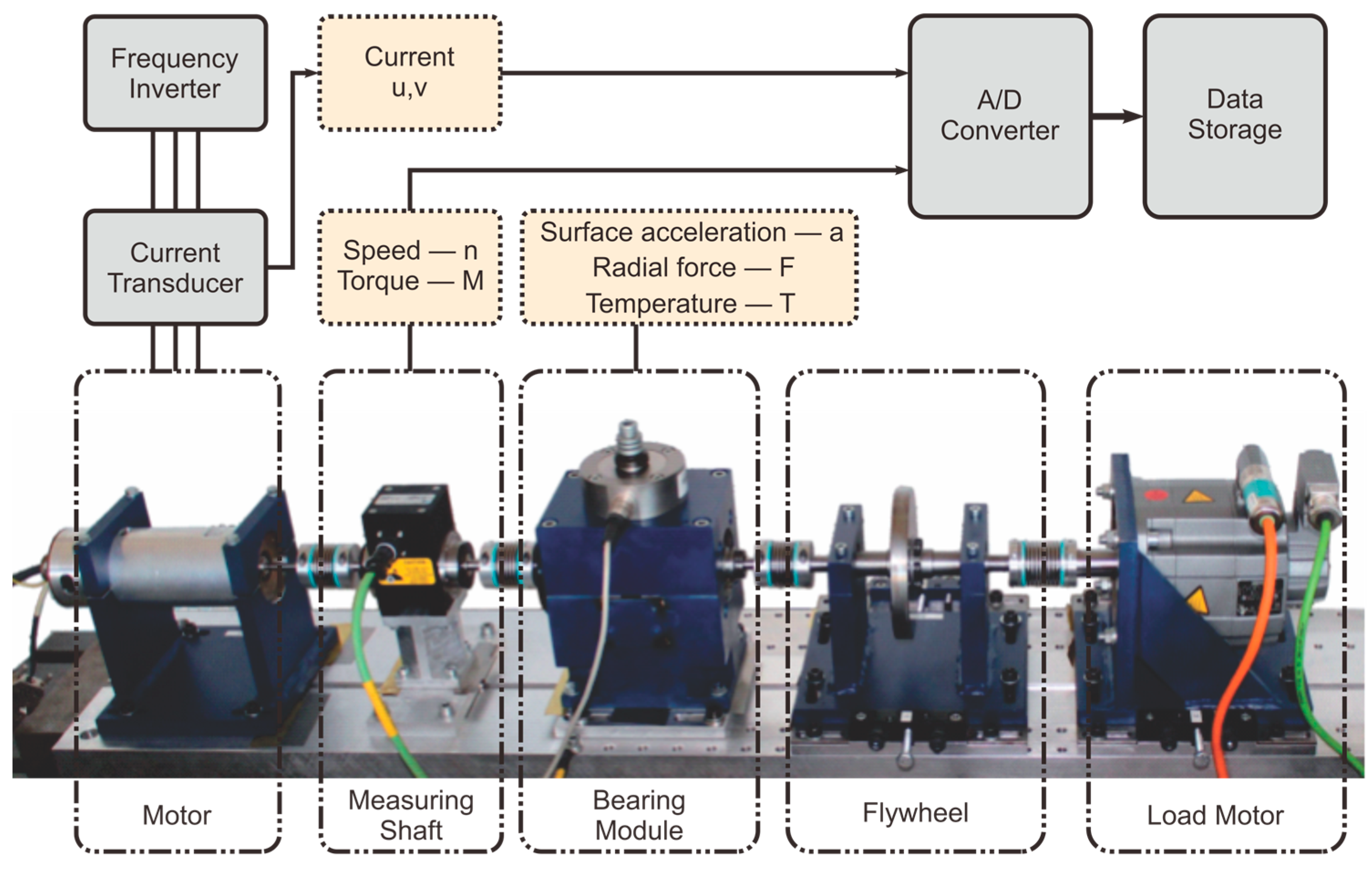
The PU dataset’s vibration data were collected using the modular experimental setup depicted in Figure 1. This experimental setup configuration includes the drive and load motor, the module for bearing installation, a flywheel, and a measuring shaft.

The drive motor used in this experimental setup is a synchronous type 425 W with a permanent magnet rotor. It is produced by Hanning Elektro-Werke GmbH & Co. KG, based in Oerlinghausen, Germany, with model code Type SD4CDu8S009. Motor control is performed using the 16 kHz switching frequency industrial inverter from KEB-automation (model name: KEB Combivert 07F5E 1D-2B0A). The module for bearing installation enables quick substitution of ball bearings with the new type of faults for each experiment without the need for time-consuming disassembly and assembly. For each bearing, a number of tests were carried out under four distinct conditions with different RPMs, load torques, and radial forces.

Table 1. Conditions of the Paderborn University test rig operation.

No.	Rot. Speed (rpm)	Load Torque (Nm)	Radial Force (N)
0	1500	0.7	1000
1	900	0.7	1000
2	1500	0.1	1000
3	1500	0.7	400

provides a comprehensive overview of the operating conditions for the study.

The vibration signal data were obtained using a piezoelectric accelerometer (Model 336C04) supplied by PCB Piezotronics Inc., a company located in Depew, NY, USA. This accelerometer was securely affixed to the upper part of the bearing module during the testing process for acceleration measurement. The dataset authors used a Type 5015A instrument for charge amplification produced by Kistler Group Winterthur, Switzerland, along with a low-pass filter with a 30 kHz cutoff frequency. The recorded signal was then digitized at a 64 kHz sampling rate, following analog-to-digital conversion. For this work, the data were cut in such a way that one dataset sample is equivalent to one second of the vibration signal. Additionally, considering that the first 10 harmonics of all estimated bearing fault characteristic frequencies in this dataset lay within the 0–1500 Hz spectrum, the data were down-sampled to the rate of 8 kHz.

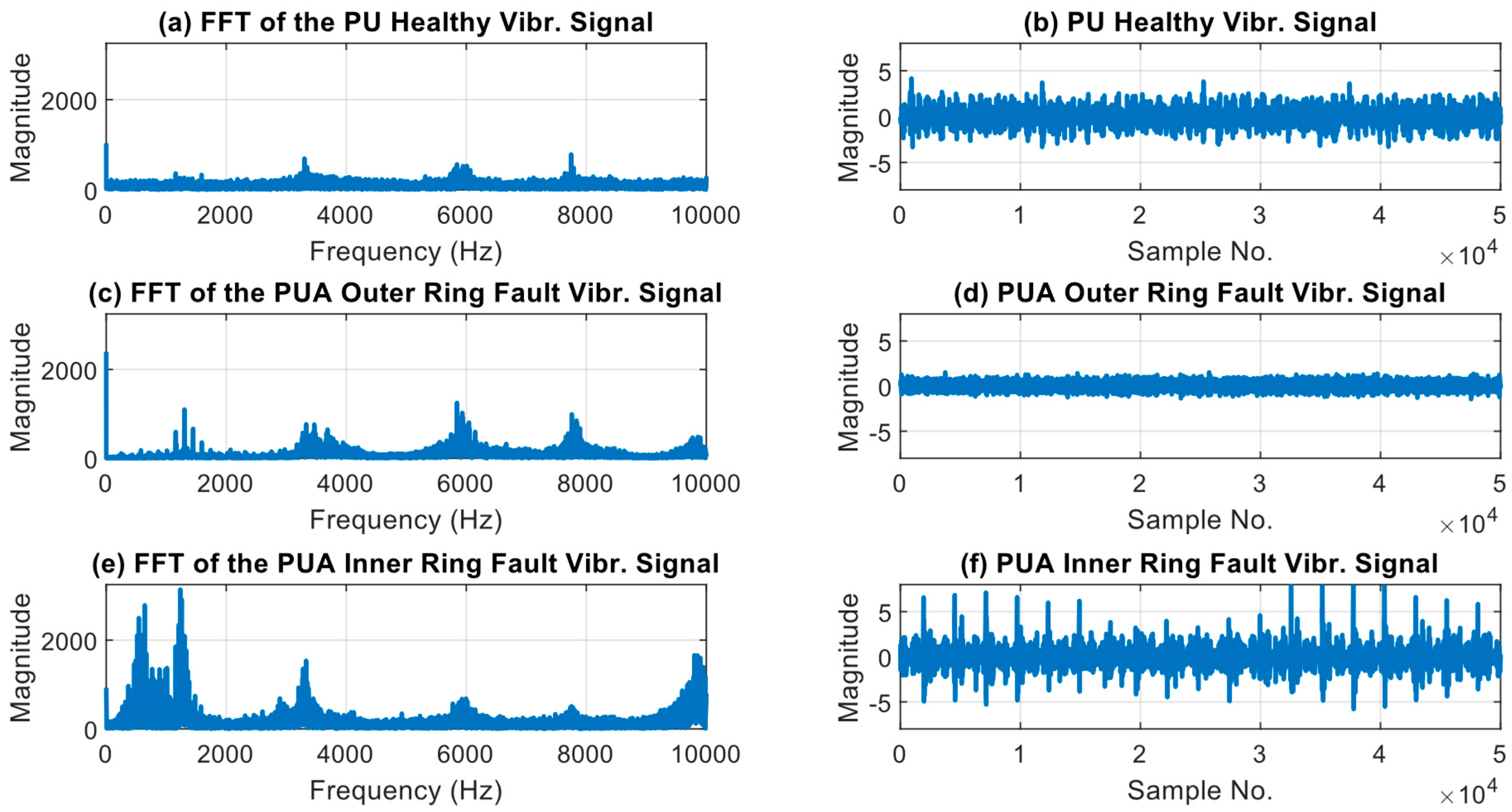
The PU dataset contains signals from six healthy bearings with a run-in period varying from 1 to 50 h. For the PUA data, the dataset authors used 12 bearings with faults inflicted using the electric discharge machine (EDM), by manual electric engraving and drilling. The EDM trenches run 0.25 mm in length along the rolling direction and have a depth of 1–2 mm. On the other hand, damages made by the manual electric engraver vary in length, ranging from 1 to 4 mm. The bearing rings have drilled holes with diameters of 0.9 mm, 2 mm, and 3 mm. The bearings are categorized into three classes based on the location of the fault: healthy, outer ring fault, and inner ring fault.

Table 2. Bearing class assignments in the PUA dataset.

Bearing Type	Bearing Code
Healthy	K: 001, 002, 003, 004, 005, 006
Outer ring damage	KA: 01, 03, 05, 06, 07, 08, 09
Inner ring damage	KI: 0, 03, 05, 07, 08

presents information about the PUA dataset arrangement. The EDM trenches are 0.25 mm in length and 1–2 mm deep. The length of the damages executed using the electric engraving tool is 1–4 mm. The holes inflicted by drilling on the inner and outer race have diameters of 0.9 mm, 2 mm, and 3 mm. All the bearings are attributed to one of three classes depending on the inflicted fault location. The arrangement of the PUA dataset with bearing codes is provided in Table 2. Time- and frequency-domain plots illustrative of all types of faults in the PUA dataset are shown in Figure 2.

2.2. Paderborn University Bearing Data with Real Damage (PUR Dataset)

For the PUR dataset, the dataset authors selected 14 bearings damaged by accelerated lifetime faults. The incurred defects were a consequence of experiments conducted on a specially engineered apparatus equipped with a spring-screw system, enabling the application of substantial radial force and emulating a natural mechanism of defect creation. Additionally, to create a more aggressive environment, the bearings were improperly lubricated using low-viscosity oil. The PUR dataset consists of 14 bearings deliberately damaged through accelerated life testing. The dataset authors achieved this by subjecting the bearings to specific tests using a specially designed machine with a spring-screw mechanism, which simulated natural fault development. To intensify the testing conditions, the bearings were improperly lubricated using low-viscosity oil, creating a more severe environment for damage induction. Damages obtained from the accelerated lifetime experiments are characterized as fatigue that appears as pitting in more than 2/3 of the cases. Damages outside of this category appear as permanent deformations manifested as indentations caused by debris. The assessment of the damage severity was performed by measuring the span of the impacted region on the ring surface along the pathway of the roller elements.

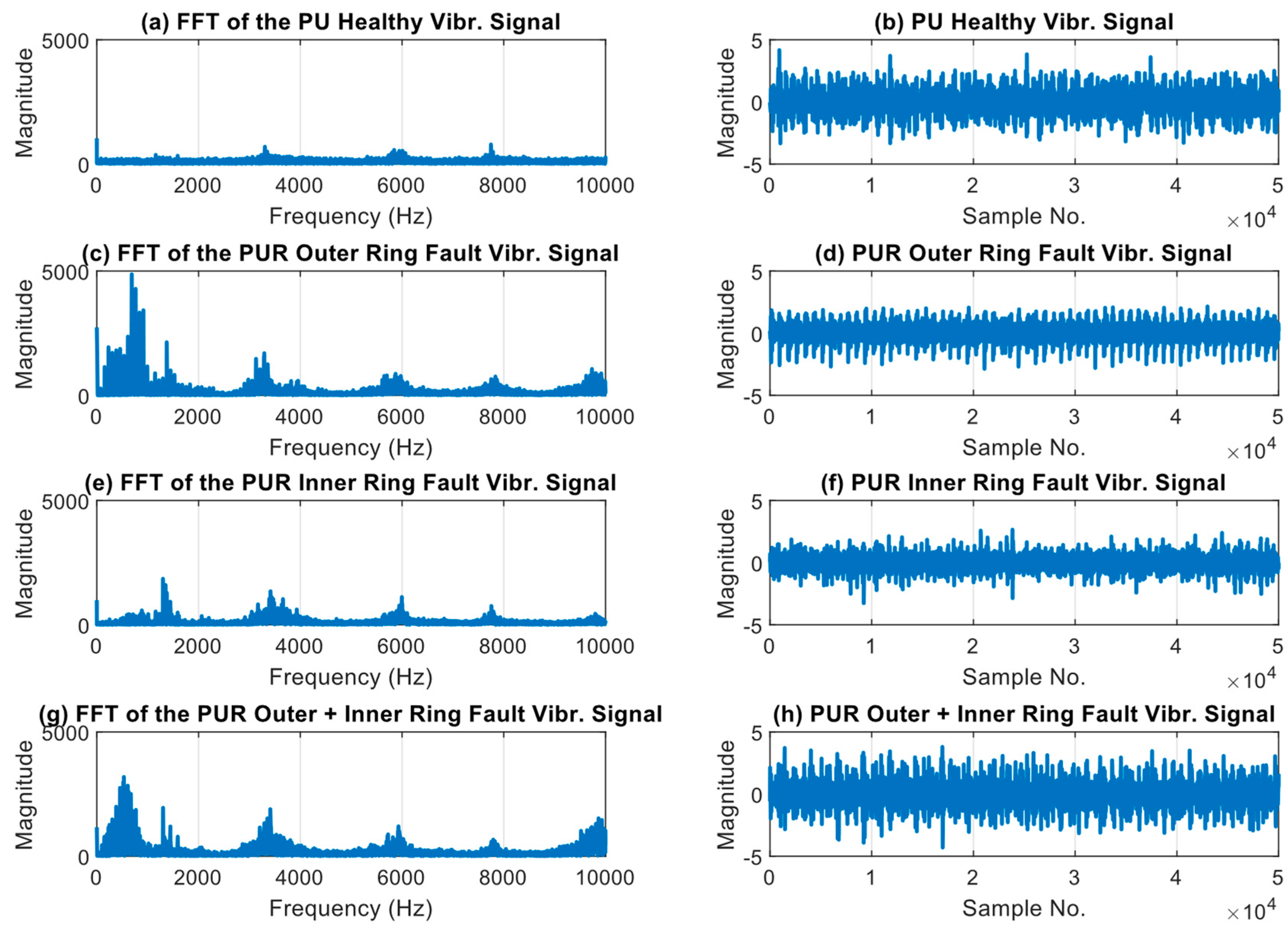
The damages were categorized into three levels depending on the ratio of the damage span to the circumference of the pitch: first level (0–2%), second level (2–5%), and third level (5–15%). Based on the location of the single damages, bearings are distinguished as having either an outer ring fault, an inner ring fault, or in the case of having both, outer + inner ring faults. The rolling elements of the bearings remained intact. The arrangement of the PUR dataset with bearing codes is provided in

Table 3. Bearing class assignments in the PUR dataset.

Bearing Type	Bearing Code
Healthy	K: 001, 002, 003, 004, 005, 006
Outer ring damage	KA: 04, 15, 16, 22, 30
Inner ring damage	KI: 04, 14, 16, 17, 18, 21
Outer + inner ring fault	KB: 23, 24, 27

. Time- and frequency-domain plots illustrative of all types of faults in the PUR dataset are shown in Figure 3.

2.3. Case Western Reserve University Bearing Data (CWRU Dataset)

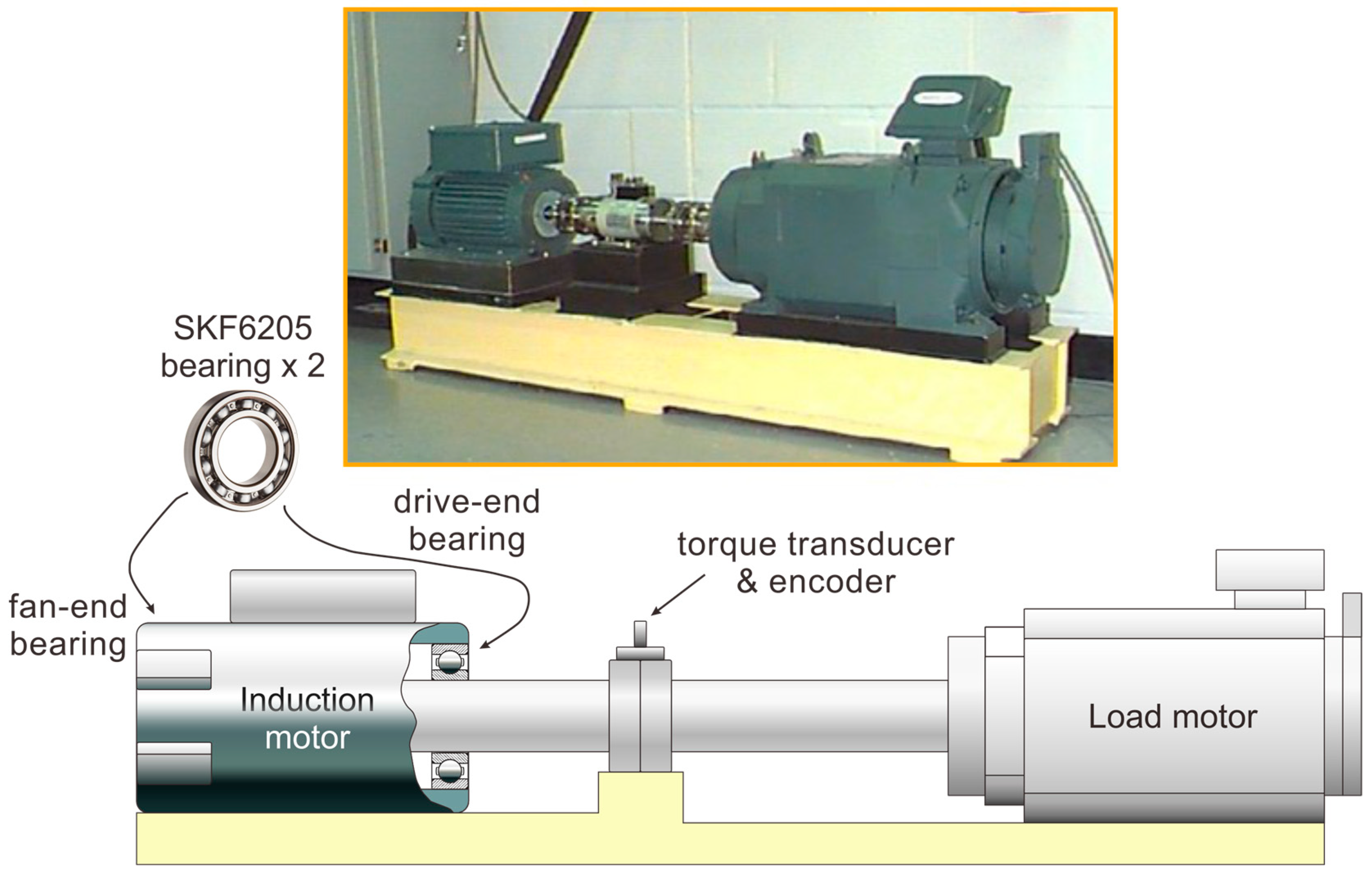
In this dataset’s testbed configuration, a 2 hp motor was utilized, and accelerometers were affixed to both the motor base and the motor itself. SKF6205 bearings were installed at the drive end and fan end of the motor, while a torque transducer was employed to collect the RPM and power data. The testbed used in the CWRU setup is depicted in Figure 4 [39].

Electric discharge machining technology was used to intentionally create faults on the bearing’s inner ring, outer ring, and rolling element. These faults have diameters between 0.007 inches and 0.040 inches. Stationary faults were induced on the outer ring. The vibration response of the setup varies depending on the fault location with respect to the load area of the bearing. To mitigate the role of this effect, experiments were performed with faults positioned at 3 o’clock, 6 o’clock, and 12 o’clock both for the bearings at the fan end and at the drive end. For each experimental run, only a single faulty bearing was installed.

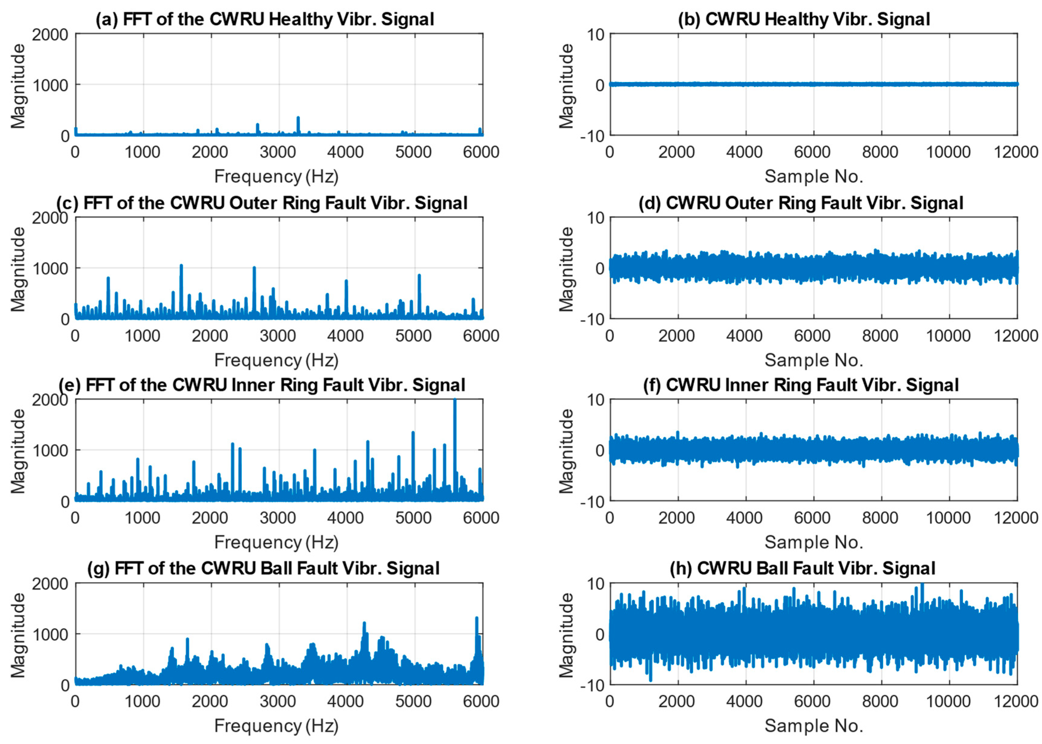
In this study, vibration data were gathered using acceleration measurements of the motor during its operation, spanning a speed range of 1720 to 1797 RPM under different load conditions ranging from 0 to 3 hp. The data were recorded using a 16-channel DAT recorder with a sampling rate of 12 kHz. Subsequently, the data were divided into one-second samples, culminating in a total set of 1920 samples. The assignment of the data to different classes was performed using bearing codes as displayed in

Table 4. Bearing class assignments in the CWRU dataset.

Bearing Type	Bearing Code
Healthy	97–100
Outer ring damage	130–133, 144–147, 156–160, 197–200, 234–237, 246–249, 258–261
Inner ring damage	056–059, 105–108, 169–172, 209–212
Ball damage	048–051, 118–121, 185–188, 222–225

. Time- and frequency-domain plots illustrative of all types of faults in the CWRU dataset are shown in Figure 5.

3. Technical Background

3.1. Wavelet Packet Transform

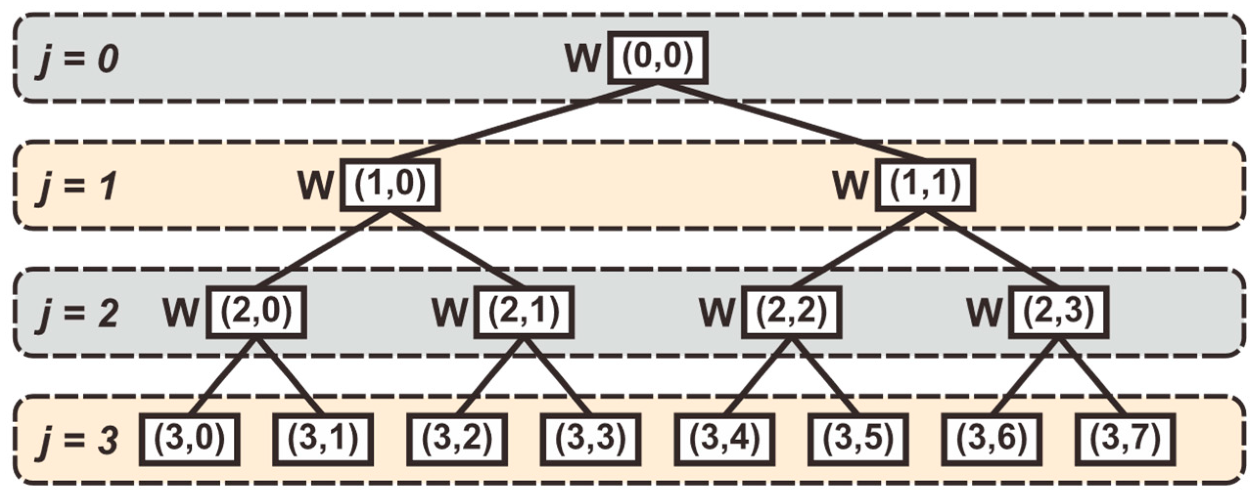
Wavelet packet transform is a more generalized method as compared to basic wavelet transform since its decomposition tree splits towards both lower and higher frequency spectra. This feature gives it the ability to characterize the non-stationary bearing fault signals. When performing signal analysis using WPT, the input signal is broken down into a collection of wavelet packet nodes arranged in a complete binary tree structure. These nodes are assigned an index in the format $(j,n)$ and their respective coefficient of wavelet packet tree is represented as $d_j^n$, in which the level of decomposition is indicated by j, while n denotes the number of nodes in that level. In the WPT structure presented in Figure 6, the input signal is located at the node indexed W(0,0), which is called the root of the WPT tree. Index W(1,0) is located at the low-pass filtered branch and W(1,1) is located at the high-pass filtered branch. These nodes result in a vector with approximation coefficients $d_1^0$ and a vector with detail coefficients $d_1^1$. Likewise, all further WPT nodes are split at every decomposition level j.

To begin WPT decomposition, it is necessary to establish the scaling function $\varphi \left(t\right)$ and the base wavelet function $\psi \left(t\right)$. The relationships between these functions can be described by a system of equations, which can be expressed as follows:

$$\{\begin{array}{l}\varphi (t)=\sqrt{2}{\displaystyle \sum _k{h}_k}\varphi (2t-k)\\ \psi (t)=\sqrt{2}{\displaystyle \sum _k{g}_k(2t-k)}\end{array}$$

(1)

where the low-pass filter is denoted as $h_k$, the high-pass filter is denoted as $g_k$, and k represents a transformation parameter.

Once the basis function is established, it is possible to implement a recursive algorithm for signal decomposition with the following definition:

$$\{\begin{array}{l}{{\displaystyle d}}_{j+1}^{2n}\left[k\right]=\sqrt{2}{\displaystyle \sum _l{h}_{l-2k}}{d}_j^n\left[k\right]\\ {{\displaystyle d}}_{j+1}^{2n+1}\left[k\right]=\sqrt{2}{\displaystyle \sum _l{g}_{l-2k}}{d}_j^n\left[k\right]\end{array}$$

(2)

where the coefficients are denoted as $d_j^n\left[k\right]$ for the wavelet packet coefficients, $d_{j+1}^{2n}\left[k\right]$ for the approximation coefficients, and $d_{j+1}^{2n+1}\left[k\right]$ for the detail coefficients. The symbol $h_{l-2k}$ stands for the low-pass filter coefficients and $g_{l-2k}$ stands for the high-pass filter coefficients.

The input signal, once decomposed through WPT, can be reconstructed using the deduced algorithm as follows:

$$d_j^n\left[k\right]={\displaystyle \sum _l{h}_{k-2l}{d}_{j+1}^{2n}\left[k\right]}+{\displaystyle \sum _l{g}_{k-2l}{d}_{j+1}^{2n+1}}\left[k\right]$$

(3)

Using a notation of $S_{j,n}$ to represent a reconstructed signal of wavelet packet coefficients $d_j^n$, the original signal can be represented as a sum of the reconstructed signals at the decomposition level $j$. With the assumption that the decomposition level $j=2$, the original signal can be represented as follows:

$$S_{0,0}=d_0^0=S_{2,0}+S_{2,1}+S_{2,2}+S_{2,3}$$

(4)

3.2. Approaches for Mother Wavelet Selection

The results of WPT decomposition heavily depend on the selection of the basis function, called the mother wavelet. Various methods for selecting the mother wavelet have been proposed, and they can be classified as qualitative or quantitative. Qualitative methods involve investigating wavelet properties, such as symmetry, orthogonality, regularity, compact support, vanishing moment, and explicit expression, to choose the one that best suits the specific task. However, relying solely on wavelet properties can be limiting because multiple wavelets may possess identical properties and parameters, making it challenging to determine the most suitable one. To address this challenge, researchers have explored an alternative qualitative approach called shape matching, which involves analyzing the geometric shape of wavelets. This approach aims to identify a mother wavelet that is similar in shape to the target signal feature component, thereby facilitating the effective extraction of signal components. Despite its potential benefits, the manual process of matching the shape of a signal with the mother wavelet can often be extremely tedious and time-consuming, as it requires manual visual comparison and lacks automation.

Extensive research has been conducted on quantitative methods with the aim of overcoming the limitations of qualitative methods. These methods employ various quantitative measures such as signal energy, Shannon entropy, cross-correlation, Emlen’s modified entropy measure, cross-correlation, and distribution error criterion to identify the most suitable mother wavelet. In recent years, among the most popular quantitative methods for mother wavelet selection, the maximum energy to Shannon entropy ratio criterion appears to be the most prevalent. It joins the popular maximum energy metric and Shannon entropy metric forming a robust and convenient method for mother wavelet selection.

The maximum energy method implies that the best-fitting mother wavelet will allow the extraction of the largest amount of energy from the signal under analysis. Its energy, with x standing for discrete-time signal, can be expressed as follows:

$$E_x={\displaystyle \sum _{n=1}^N{\left|x_n\right|}^2}$$

(5)

However, it is noteworthy that signals with equal energy may exhibit varying frequency distributions. Specifically, one signal may display higher energy levels of frequency components significant for feature selection, while another may have a broad spectrum with a flat energy level across the whole spectrum, lacking practicality for fault diagnosis. To quantitatively express the signal energy distribution among WPT nodes at the decomposition layer, Shannon entropy is used and calculated as follows:

$$H=-{\displaystyle \sum _{i=1}^N{p}_i\cdot {\log }_2{p}_i}$$

(6)

where $p_i$ is the energy probability distribution of the wavelet coefficients. Considering wt(s, i) is the i^th coefficient at the s level, then $p_i$ is defined in the following manner:

$$p_i=\frac{{\left|wt(s,i)\right|}^2}{E_x(s)}$$

(7)

Thus, the energy-to-Shannon entropy ratio can be defined as follows:

$$R(s)=\frac{E_x(s)}{H(s)}$$

(8)

Using Equation (8), the $R\left(s\right)$ ratio is calculated at the necessary WPT decomposition level for every candidate mother wavelet. The candidate wavelet with the highest value of energy to Shannon entropy is selected as the base for the WPT decomposition of the given signal or set of signals.

3.3. Linear Discriminant Analysis

Linear discriminant analysis (LDA) is a powerful supervised dimensionality reduction tool. It works by projecting high-dimensional data onto a lower-dimensional space while maintaining the original class information. To obtain the ideal class discrimination matrix, the algorithm seeks to minimize the scatteredness within a class while maximizing the distance between classes. In multiclass LDA, the within-class variance $S_W$ matrix can be represented in the following way:

$$SW={\displaystyle \sum _{j=1}^c{\displaystyle \sum _{i=1}^{n_j}\left(x_{ij}-{\mu }_j\right)}{\left(x_{ij}-{\mu }_j\right)}^T}$$

(9)

where $S_W$ is the within-class variance, ${\mu }_j$ is the mean of $j_{\mathrm{t}\mathrm{h}}$ class, $x_{ij}$ is the $i_{\mathrm{t}\mathrm{h}}$ sample of the $j_{\mathrm{t}\mathrm{h}}$ class, c is the total number of classes, and $n_j$ is the number of samples in the class.

$$SB={\displaystyle \sum _{j=1}^c{n}_i\left({\mu }_i-\mu \right){\left({\mu }_i-\mu \right)}^T}$$

(10)

where $S_B$ is the between-class variance, ${\mu }_i$ is the mean of $i_{\mathrm{t}\mathrm{h}}$ class, and $\mu$ is the total mean.

After $S_W$ and $S_B$ are calculated, the transformation matrix $W$ of the LDA technique that maximizes Fisher’s criterion formula in Equation (11) can be expressed as Equation (12).

$$\underset{W}{\arg \max }\frac{W^T{S}_{B}W}{W^T{S}_{W}W},\begin{array}{cc}& (S_{W}W=\lambda \end{array}{S}_{B}W)$$

(11)

$$W=S_W{}^{-1}{S}_B$$

(12)

For the transformation matrix $W,$ the generalized eigenvalue problem is solved to obtain the axes of the LDA space in the form of eigenvectors $V$ and their eigenvalues $\lambda$. The eigenvectors represent the directions of the new space, and the eigenvalues represent their robustness or their ability to discriminate between classes. Thus, only $k$ eigenvectors with the highest eigenvalues are selected to construct the final lower dimensional space. After that, the original data are projected onto the LDA space. Assuming that $M$ is the number of dimensions in the original data, then $(M-k)$ dimensions are removed from each sample. Now each point of the original data will be represented in the k-dimensional space, and the projection can be defined as follows:

$$Y=X{V}_k$$

(13)

where $X$ is a data matrix, $V_k$ is the lower dimensional space, and $Y$ is the data matrix after projection.

4. Proposed Method

4.1. Vibration Signal Processing

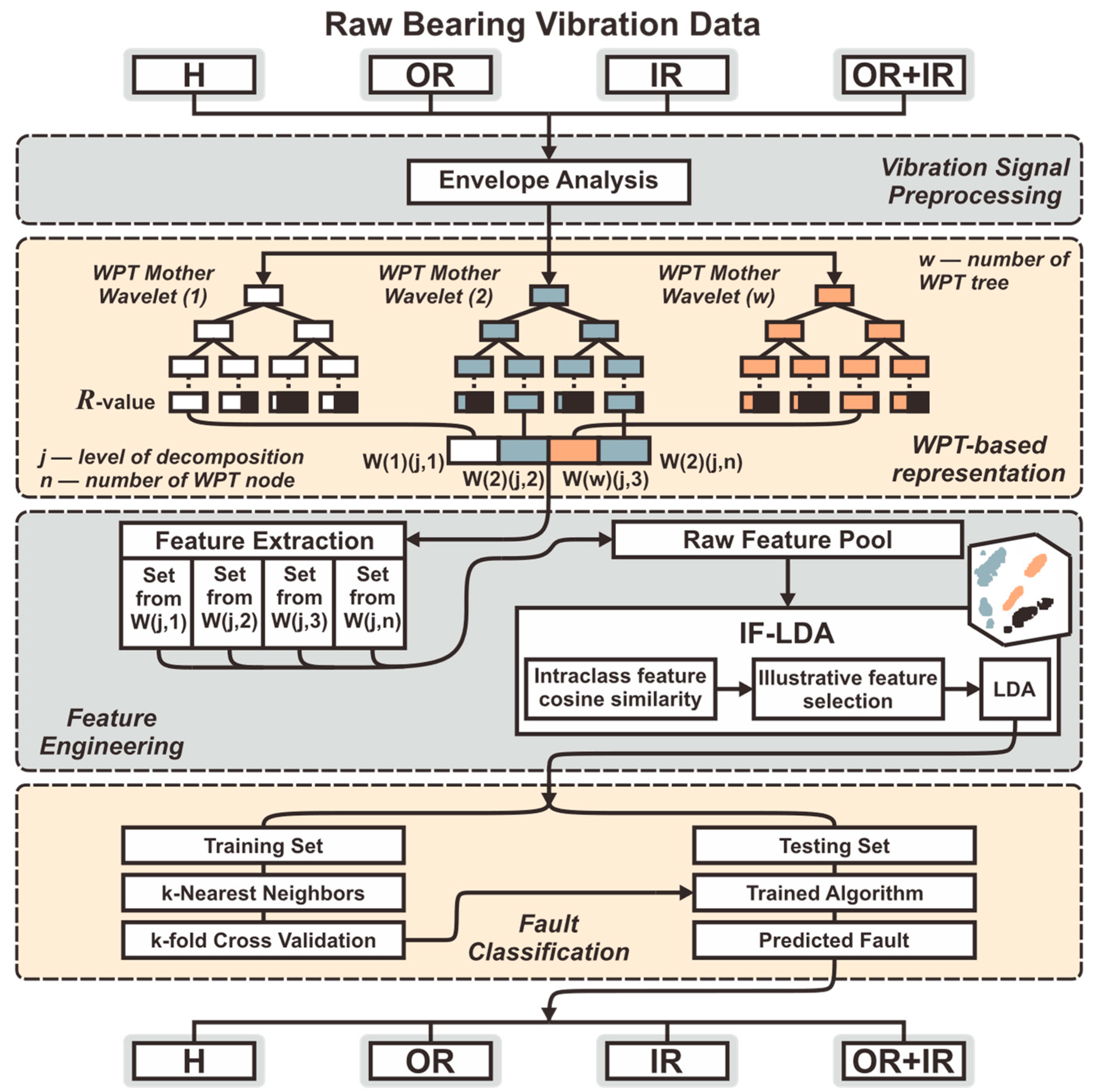
Faulty bearings produce high-frequency components in the vibration signal due to various mechanisms, such as impact, rubbing, or resonance. These high-frequency components are often masked by low-frequency components in the signal, such as those caused by machine operation, background noise, or measurement noise. For this reason, a signal processing technique known as envelope analysis is applied for signal preprocessing in order to extract the high-frequency components of a signal by use of demodulation. Thus, as can be seen from the workflow of the proposed method in Figure 7, the raw signal is initially preprocessed using Hilbert transform envelope extraction.

This is completed by taking the module of the analytical signal obtained from the Hilbert transform. The whole process can be described mathematically starting with Equation (14), which reveals the expression of the vibration signal $x\left(t\right)$, where the amplitude modulation envelope is given by $A\left(t\right)$ and the function of phase modulation is represented by $\phi \left(t\right)$.

$$x(t)=A(t)\cos (2\pi ft+\phi (t))$$

(14)

The transformation of x(t) via the Hilbert transform is demonstrated in Equation (15) as its 90-degree phase shift.

$$\widehat{x}(t)=A(t)\sin (2\pi ft+\phi (t))$$

(15)

The ensuing analytical signal is obtained as a complex number:

$$Z(t)=x(t)+j\widehat{x}=A(t)e^{j\phi (t)};$$

(16)

By computing the modulus of $Z\left(t\right)$, the envelope of the signal can be determined as follows:

$$\left|Z(t)\right|=A(t)$$

(17)

4.2. Vibration Signal Processing

The choice of a mother wavelet when decomposing a signal using the wavelet packet transform (WPT) can have a significant impact on the spectral characteristics of the resulting coefficients. Different mother wavelets may be better suited for capturing specific types of spectral content or signal features, while others may not be as effective. In the regular WPT procedure explained in Section 3.2, a list of various mother wavelets is available for selection. To evaluate the effectiveness of the mother wavelets, a representative subspace of the signal data is chosen. This subspace is decomposed using each mother wavelet from the list, creating a unique WPT tree for each one. Then, the reconstructed coefficients at the desired decomposition level are assessed for each tree. The mother wavelet that exhibits the best evaluation score in comparison to the other wavelets is selected for the decomposition of the entire dataset.

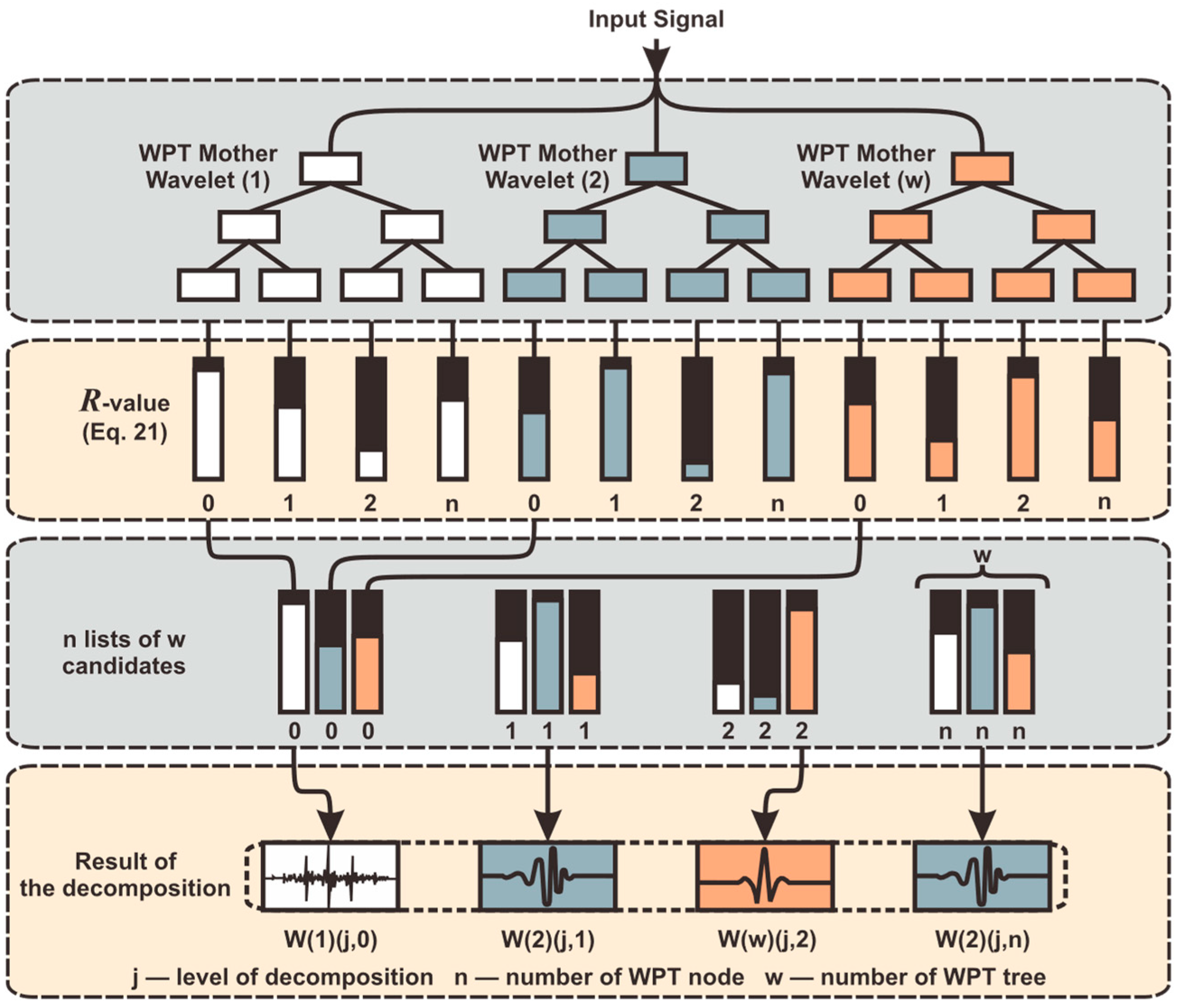
The proposed WPT-based signal representation, on the other hand, provides a different approach. This method aims to represent a signal using WPT decomposition as a foundation, but it is not limited to using a single mother wavelet. Firstly, the given signal data are decomposed to the level j (which in this work equals to j =3) using the set of W mother wavelets resulting in W WPT trees. Following that, at the desired decomposition level, the nodes with the same indexes from $d_j^0$ to $d_j^n$ are taken for comparison across the $W$ WPT trees forming a list of candidates with a dimension of $1\times W$, which in this work is $1\times 36$ since $W=36$ wavelet functions were tried. For each of the candidate lists, the assessment is performed based on the spectral content evaluation of each reconstructed WPT coefficient, which is calculated using the ratio of the total power of the spectrum and the Shannon entropy of the signal power spectrum. The workflow of the novel WPT-based signal representation is shown in Figure 8.

Considering the definition of Shannon entropy of signal power spectrum:

$$H_{ps}=-{\displaystyle \sum _{i=1}^N{p}_i{\log }_2\left(p_i\right)}$$

(18)

where N is the total number of frequency bins in the power spectrum, and p_i is the probability of the signal power being in the frequency bin, which is defined as follows:

$$p_i=\frac{P_i}{{\displaystyle {\sum }_{j=1}^N{P}_j}}$$

(19)

where P_i is the power in the i-th frequency bin.

The total power of the signal spectrum is calculated as follows:

$$P_{ss}={\displaystyle \sum _{i=1}^N{P}_i}$$

(20)

The ratio is defined as follows:

$$R=\frac{P_{ss}}{H_{ps}}=\frac{{\displaystyle {\sum }_{i=1}^N{P}_i}}{-{\displaystyle \sum _{i=1}^N\frac{P_i}{{\displaystyle {\sum }_{j=1}^N{P}_j}}{\log }_2\left(\frac{P_i}{{\displaystyle {\sum }_{j=1}^N{P}_j}}\right)}}$$

(21)

Evaluation of the reconstructed coefficients of the WPT node using the R-value makes it possible to compare the spectral content captured by each mother wavelet and choose the one that provides the best representation of the signal within the frequency range of a particular WPT node. Specifically, the criterion measures the amount of information in the signal power spectrum that is being concentrated in specific frequency bands, as opposed to being distributed uniformly over the entire spectrum. A mother wavelet that produces a reconstructed coefficient with a higher ratio of total power to Shannon entropy is preferred, as it indicates a signal with a more predictable and more structured spectral composition.

The proposed method assembles the final decomposition of the signal node by node, depending on the R-value of its reconstruction. Different parts of the signal may have distinct spectral characteristics, and by selecting a specific mother wavelet for the decomposition of each node, the novel WPT-based signal representation can capture the relevant spectral features of the signal more accurately. It can better acquire the spectral content of the signal and identify important discriminant features, resulting in improved performance as compared to WPT which relies on the traditional mother wavelet selection methods and uses a single mother wavelet for the entire signal.

It is worth mentioning that the proposed signal representation method is based on the same principles as WPT. It does not satisfy some of the basic properties of wavelet decomposition, such as the superposition property or conservation of energy. Therefore, it cannot be considered an advanced version of WPT. However, the proposed signal representation method can still be used effectively as a feature extraction tool. The manipulations performed on the signal using the proposed signal representation method have a solid basis and are based on sound mathematical principles. As a result, the extracted features can provide useful information about the signal, which can be used for a wide range of applications, such as signal processing, classification, and pattern recognition.

4.3. Feature Extraction and Feature Pool Configuration

Collecting real-world data necessary for the diagnosis of bearing faults, including vibration data, acoustic emission data, or electric current data, involves extended periods of high-rate sampling. This process generates complex datasets with numerous variables, placing a significant demand on memory and computational resources. As a result, applying ML techniques to unprocessed data is restricted in practicality. Feature extraction is a technique that addresses this challenge by reducing the dimensionality of data. It involves the conversion of a raw dataset to a smaller one by means of extraction of high-quality features representative of the whole dataset, which contributes to superior generalization and prevents overfitting. A set of features obtained after extraction is conventionally referred to as the feature vector.

Existing literature on bearing fault diagnosis encompasses a substantial number of features that are utilized in varying permutations to establish a condensed depiction of the vibration data. In the current work, a total set of 19 features was extracted from the WPT-reconstructed node signals. Out of them, 16 are time-domain and three are frequency-domain features. These statistical features are ubiquitous in the field of bearing fault diagnosis, and anticipating the significance of specific features for fault diagnosis before feature selection is tedious. Consequently, the collection of features aggregated for this study aims to incorporate as many statistical features as feasible from the literature. The feature names along with the equations are displayed in

Table 5. Statistical features definitions.

Feature Name	Equation	Feature Name	Equation
Peak value	$X_p=\underset{i}{\max }\left|x_i\right|$	Entropy	$H(x)=-{\displaystyle \sum _{i=1}^{N}P\left(x_i\right)}\cdot {\log }_{2}P\left(x_i\right)$
RMS	$X_{RMS}=\sqrt{\frac{1}{N}{\displaystyle \sum _{i=1}^N{{\displaystyle x}}_i^2}}$	Mean	$\mu =\frac{1}{N}{\displaystyle \sum _{i-1}^N{x}_i}$
Kurtosis	$X_{kurtosis}=\frac{1}{N}\left(\frac{{\displaystyle \sum _{i=1}^N{\left(x_i-\mu \right)}^4}}{{\sigma }^4}\right)$	Skewness	$X_{kurtosis}=\frac{1}{N}\left(\frac{{\displaystyle \sum _{i=1}^N{\left(x_i-\mu \right)}^3}}{{\sigma }^3}\right)$
Crest factor	$C_f=\frac{X_p}{X_{RMS}}$	Shape factor RMS	$S{F}_{RMS}=\frac{X_{RMS}}{\mu }$
Clearance factor	$L=\frac{X_p}{{\left(\left(1/N\right){\displaystyle \sum _{i=1}^N\sqrt{\left|x_i\right|}}\right)}^2}$	Peak-to-peak value	$x_{ptp}=\max \left|x\right|-\min \left|x\right|$
Impulse factor	$L=\frac{\max \left\{\left|x_i\right|\right\}}{\left(\left(1/N\right){\displaystyle \sum _{i=1}^N\left|x_i\right|}\right)}$	Energy of signal	$e={\displaystyle \sum _{i=1}^N{x}_i^2}$
Root variance frequency	$RVF=\sqrt{\frac{{\displaystyle \underset{0}{\overset{\infty }{\int }}{(f_i-FC)}^{2}s\left(f_i\right)df}}{{\displaystyle \underset{0}{\overset{\infty }{\int }}s\left(f_i\right)}df}}$	RMS frequency	$RMSF=\sqrt{\frac{{\displaystyle \underset{0}{\overset{\infty }{\int }}{f}_i^{2}s\left(f_i\right)df}}{{\displaystyle \underset{0}{\overset{\infty }{\int }}s\left(f_i\right)}df}}$
Square mean root	$X_{SMR}={\left(\frac{{\displaystyle \sum _{i=1}^N\sqrt{x_i}}}{N}\right)}^2$	Frequency center	$FC=\frac{{\displaystyle \underset{0}{\overset{\infty }{\int }}fs\left(f\right)df}}{{\displaystyle \underset{0}{\overset{\infty }{\int }}s\left(f\right)}df}$
5th normalized moment	$HOMn5=\frac{\frac{1}{n}{\displaystyle \sum _{i=1}^N{\left(x_i-\mu \right)}^5}}{{\left(\sqrt{\frac{1}{N-1}{\displaystyle \sum _{i=1}^N{\left(x_i-\mu \right)}^2}}\right)}^5}$	6th normalized moment	$HOMn6=\frac{\frac{1}{n}{\displaystyle \sum _{i=1}^N{\left(x_i-\mu \right)}^6}}{{\left(\sqrt{\frac{1}{N-1}{\displaystyle \sum _{i=1}^N{\left(x_i-\mu \right)}^2}}\right)}^6}$
Shape factor SMR	$S{F}_{SMR}=\frac{X_{SMR}}{\mu }$

. These 19 features extracted from 8 reconstructed WPT coefficients form a row of 152 features for each sample and together constitute a primary feature pool.

4.4. Feature Extraction and Feature Pool Configuration

LDA is a dimensionality reduction algorithm without inherent feature selection capabilities. This means that input data of low quality provided to an LDA can degrade its performance for a number of reasons. Firstly, the presence of the low-quality features introduces noise and causes distortions in inter-class and between-class mean values, ergo, causes distortions in transformation matrix eigenvalues and eigenvectors resulting in suboptimal LDA space, which leads to poor classification results. Secondly, with a higher number of features, LDA will have to perform more computations due to the possibility of a larger data matrix having more linear discriminants, making the model more time-consuming. In order to avoid these issues and prevent the presence of low-quality features, LDA requires selective feature preprocessing.

In this work, selective preprocessing is performed based on the feature informative factor (IF). Initially, the cosine similarity for each pair of features in the primary vector is calculated. If features in the pair are defined as $F_i$ and $F_j$, then their cosine similarity can be defined as follows:

$$C_{sim}\left(F_i,F_j\right)=\frac{F_i\cdot F_j}{\Vert F_i\Vert \Vert F_j\Vert }$$

(22)

An informative factor metric for each feature $F_i$ is calculated as a sum of the cosine similarities of this feature with every other feature in the set as follows:

$$I={\displaystyle \sum _{i=1}^n{C}_{sim}}$$

(23)

Based on the IF, the feature is included in the informative feature pool if its magnitude is above zero or is left in the primary feature pool if its magnitude is below zero, according to the following definition:

$$I=\{\begin{array}{c}\forall F_i\begin{array}{c}\end{array}\mathrm{if}\begin{array}{c}\end{array}{I}_{value}>0,\begin{array}{c}\end{array}\mathrm{informative}\begin{array}{c}\mathrm{pool}\end{array}\\ else,\begin{array}{c}\end{array}\mathrm{primary}\begin{array}{c}\end{array}\mathrm{pool}\end{array}$$

(24)

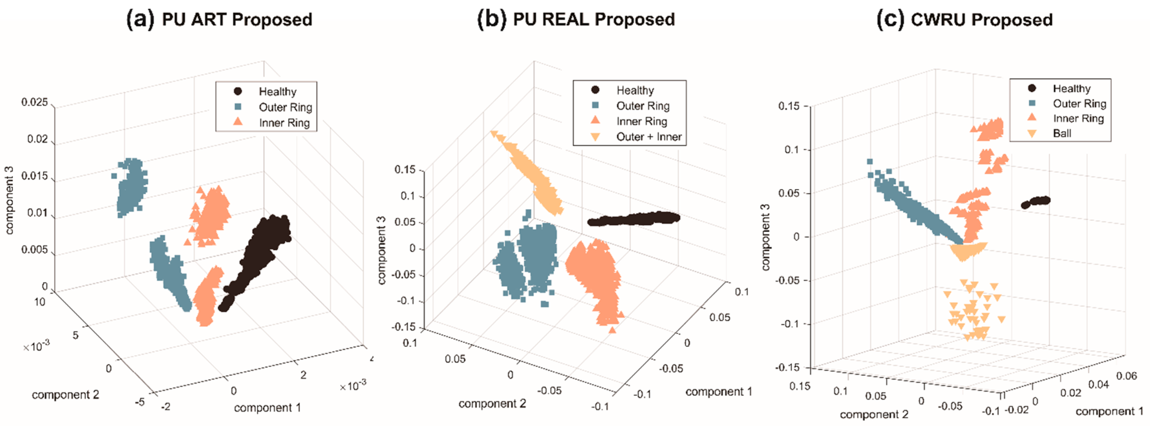
The resulting informative feature pool then undergoes the LDA transformation as was described in Section 3.3. The application of informative factors offers significant benefits for linear discriminant analysis in that it ensures a minimal level of scatteredness among the features within the same class. Overall, the application of IF-LDA for dimensionality reduction offers significant benefits for effective bearing fault diagnosis. It enables the creation of a feature space that maximizes the separation between different classes while simultaneously ensuring a dense configuration among the features within the same class. This improvement in feature space facilitates enhanced accuracy in model predictions and ensures easy generalization, leading to a more robust and reliable diagnosis. A visual representation of the high-quality feature spaces with well-separated classes obtained from using the proposed method on three different datasets is shown in Figure 9.

4.5. Bearing Fault Classification

After the feature vector dimensionality is reduced using IF-LDA, the classification of the bearing state is performed by the k-nearest neighbor (KNN) classifier. The KNN classifier is a non-parametric machine learning classification method. It determines the class membership of an input data point by finding the k closest labeled data points using a distance metric. KNN does not construct a model based on training data and, thus, is considered instance-based. Once KNN receives a new data sample $x\prime$ for classification, it calculates the distances d from this sample to the known labeled samples $x_i$. Then, based on majority voting, the new sample is allotted to the class with the highest number of instances among $k$-nearest samples in the training dataset. In this work, the number of nearest neighbors was set to $k=5$.

The effectiveness of the KNN classifier heavily relies on the quality of the features used. By leveraging the distance-based approach, KNN measures the similarity between instances based on their feature vectors. If the features effectively capture the relevant patterns and characteristics of the data, KNN can successfully identify similar instances and make accurate predictions. On the other hand, if the features are not informative or do not capture the underlying structure of the data, KNN’s performance may be limited. Therefore, the choice and quality of features play a crucial role in the success of KNN. This allows for a comprehensive assessment of the impact of different feature engineering techniques on classification accuracy. As a result, the KNN classifier serves as a robust benchmark for the evaluation of the effectiveness and generalizability of different feature engineering methods.

5. Experimental Results and Discussion

In this section, the evaluation of the bearing fault diagnosis performance is conducted on three datasets previously described in Section 2: The PUA is categorized into three classes and 5760 samples in total, the PUR dataset is categorized into four classes with 6400 samples in total, and the CWRU dataset with four class labels and 1920 total samples. To ensure fairness in the evaluation, the datasets are split in a way that 80% of data are reserved for training and 20% are reserved for testing. The validation is carried out using the 10-fold cross-validation strategy. This strategy involves randomly reordering and partitioning the data into 10 groups. During each iteration, one group is assigned as the validation data, while the remaining nine groups are utilized for training. This process is repeated 10 times, ensuring that each data sample is included in a single holdout set.

Macro-averaged (MA) recall, macro-averaged precision, F1-score, fault identification accuracy, and one-class true positive rate were used as metrics for performance comparison and their definitions are provided in Equations (25)–(29), where TP stands for true positive, FN for false negative, FP for false positive, the lowercase $k$ stands for the class number, the capital $K$ stands for the total number of classes, and $N$ is the total number of samples.

$$Re{c}_m=\frac{1}{K}\left({\displaystyle \sum _{k=1}^K\frac{{{\displaystyle TP}}_k}{{{\displaystyle TP}}_k+{{\displaystyle FN}}_k}}\right)\times 100$$

(25)

$$Pre{c}_m=\frac{1}{K}\left({\displaystyle \sum _{k=1}^K\frac{T{P}_k}{T{P}_k+F{P}_k}}\right)\times 100$$

(26)

$$F{1}_m=2\times \left(\mathrm{Pr}e{c}_m\times \mathrm{Re}{c}_m\right)/\left(\mathrm{Pr}e{c}_m+\mathrm{Re}{c}_m\right)$$

(27)

$$FIA=\frac{{\displaystyle {\sum }_k^{K}T{P}_k}}{N}\times 100,$$

(28)

$$TP{R}_k=\left(\frac{{{\displaystyle TP}}_k}{{{\displaystyle TP}}_k+{{\displaystyle FN}}_k}\right)\times 100$$

(29)

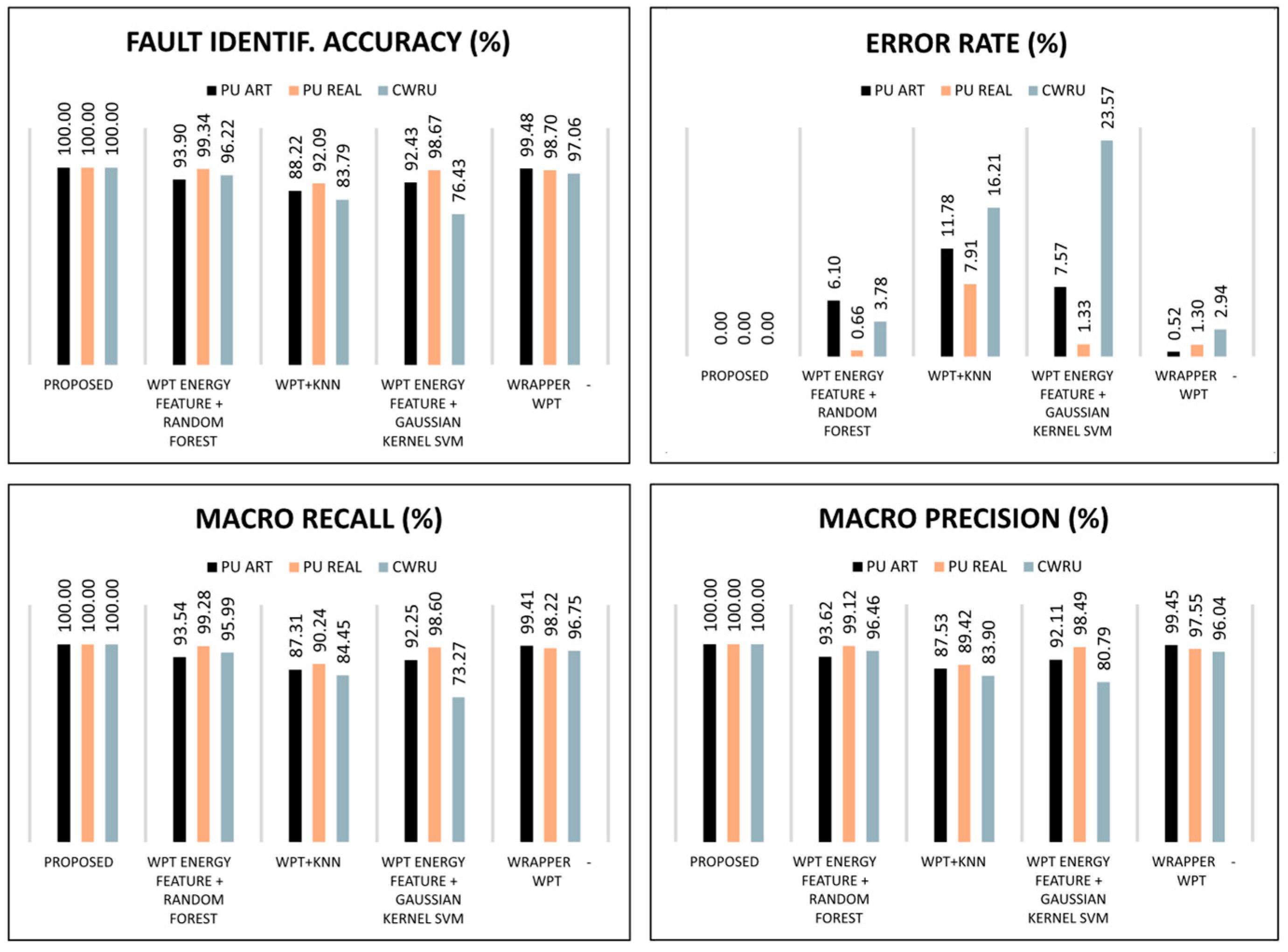
The methods selected for comparison have a similar nature to the proposed method in terms of bearing vibration signal processing. This relatedness helps to correctly evaluate the increase in fault diagnosis performance introduced by the proposed method. All the calculated metrics are represented as column charts in Figure 10 and Figure 11 for convenient comparison.

Applying the proposed method to the PUR, PUA, and CWRU datasets resulted in an FIA of 100% for each dataset. Accordingly, the error rate equals 0% for each dataset and MA recall and MA precision are 100%. The results obtained from the proposed method can be explained by the quality of the WPT-based signal representation, where each node is chosen according to the R-value criterion, ensuring that the reconstructed signals possess a well-defined spectrum with prominent high-energy frequency components and minimal interference from noise. This allows for avoiding the effect of noisy or corrupted reconstructed signals in certain nodes for the reason of the low sensitivity of a particular mother wavelet to the shape of the components in the frequency range of the particular WPT node. Another reason for the high performance of the proposed method lies in the IF-LDA dimensionality reduction technique. The informative factor (IF) selective feature preprocessing helps to eliminate low-quality features that have poor correlation with the dependent variables. This step is crucial to prevent degradation of the performance of the LDA. Moreover, the features accepted into the final pool using IF preprocessing are compactly clustered within the same class and exhibit a high inter-class difference in mean value. Therefore, after reducing the dimensionality with LDA, the feature space depicted in Figure 9 is obtained. Given the resulting feature space that exhibits distinct boundaries between classes, maximizing the distinction between healthy bearings and various fault states, a simple KNN model is fully capable of achieving 100% fault diagnosis performance, as assessed using several metrics presented in Figure 7 and Figure 8.

The first comparison method uses the signal energy features extracted from wavelet packet bases to train the random forest classifier [40]. Utilizing WPT for signal energy feature extraction has become a widely used reliable strategy in the fault diagnosis field. Together with a powerful random forest algorithm, this method showed high performance on three datasets. Nevertheless, by solely relying on energy features in contrast to a diverse vector of features derived from both the time domain and the frequency domain, the method fails to capture the necessary level of distinctiveness and falls behind the proposed method. Thereby, the FIA demonstrated by this method on the PUA set is 93.90%, 99.34% for the PUR set, and 96.22% for the CWRU set. Accordingly, the error rates are 6.10%, 0.66%, and 3.78%. The MA recall values are 93.54%, 99.28%, and 95.99%, respectively, and the MA precision values are 93.62%, 99.12%, and 99.46%, respectively. In addition, while node energy features may indicate changes in overall energy levels, they do not offer insights into the specific fault-related patterns that can be crucial for accurate diagnosis.

The second comparison method [41] employed a similar approach by utilizing the WPT for bearing vibration signal decomposition. The extracted features described in Section 4.2 were used to train a KNN classifier. This method demonstrated inadequate performance when diagnosing compound bearing faults and exhibited mediocre abilities in fault diagnosis. In particular, the FIA values for the three datasets achieved by this method are 88.22%, 92.09%, and 83.79%, respectively, which correspond to the error rates of 11.78%, 7.91%, and 16.21%. The MA recall values are 87.31%, 90.24%, and 84.45%, respectively, and the MA precision values are 93.62%, 99.12%, and 96.46%, respectively. One of the contributing factors to this subpar performance is the absence of feature selection. Without it, random fluctuations in the data and noisy features which contain minimal discriminant information or exhibit weak correlation with the response may cause the model to overfit to these instances and eventually cause poor fault diagnosis performance and misclassification.

The third comparison method, which utilizes a robust Gaussian kernel SVM classifier, exhibited poor performance due to its heavy reliance on WPT energy features, analogously to the first comparison method [42]. The FIA values for the three datasets are 92.43%, 98.67%, and 76.43%, respectively, which correspond to error rates of 7.57%, 1.33%, and 23.57%. The MA recall values are 92.25%, 98.60%, and 73.27%, respectively, and the MA precision values are 92.11%, 98.49%, and 80.79%, respectively.

The performance levels of the last comparison method are very high and are the closest to the proposed method [43]. The FIA values achieved by this method on the three datasets are 99.48%, 98.70%, and 97.06%, respectively, while the error rates are 0.52%, 1.30%, and 2.94%, respectively. The MA recall metrics are equal to 99.41%, 98.22%, and 96.75%, respectively, while the MA precision values are 99.45%, 97.55%, and 96.04%, respectively. This can be explained by the utilization of the Boruta feature selection algorithm, which evaluates each feature in the set depending on its usability for the random forest (RF) classifier. Boruta uses random permutations of the features called shadow attributes (SA) and attaches them to the feature vector to create the extended information system (EIS). RF is trained on EIS multiple times, each time with new SA permutations. After each training iteration, the model is tested, and the calculation of the correct class votes is calculated. Eventually, only the features that are significantly more useful than any of its own permutations are selected for the final feature set. The rest of the features are neglected. This allows for constructing a feature set with highly discriminant features that enables reliable FD performance of the method using the KNN model.

Given the data parameters described in Section 2, the proposed method is capable of diagnosing the type of fault in the bearing under analysis in 0.3 to 0.33 s when running on a PC equipped with an Intel^® Core™ i7-9700K CPU and 16 GB of RAM.

6. Conclusions

This paper proposed a method for bearing fault diagnosis using a novel WPT-based signal representation and informative factor LDA. The shape of the mother wavelet that poorly matches the shape of the signal components along the spectrum may cause inconsistent results of the decomposition with a low level of detail. Having decomposed the signal using various mother wavelets, the proposed R-value criterion based on the energy-to-entropy value of the node reconstruction allows the model to tailor a representation consisting of the nodes decomposed using mother wavelets that allow the extraction of the highest amount of detail and bearing fault-related information at the local frequency spectrum contained in the WPT node.

The dimensions of the vector of features extracted from this representation are reduced using the proposed informative factor LDA. The informative factor preprocesses the features, retaining only those that exhibit dense clustering within each class and offer optimal inter-class separation. The IF provides LDA with the advantage of early elimination of noisy and low-quality features, protecting LDA from outliers and enhancing interclass separability. Moreover, it reduces the computational time by providing a smaller feature vector matrix, which results in fewer possible LDA spaces. Overall, the introduction of an informative factor results in excellent LDA performance and complete class separation in the LDA space. For classification, the KNN algorithm was used, and the results surpassed those obtained by all other comparison methods.

It is worth noting that the advantages of the WPT-based signal representation, while promising, do come with a slight increase in computational time during training. This arises from the need to assess the quality of signal decomposition using various mother wavelets. To mitigate this, employing a smaller portion of the overall dataset as well as refining and reducing the mother wavelet candidate list through benchmark comparisons across diverse datasets can be beneficial. In light of these considerations, a future work direction could involve a benchmark comparison method that permanently eliminates the poorest-performing wavelets from the candidate list. Another potential avenue for future work is adapting the proposed algorithm to handle bearing fault data with transient rotational speeds.

References

1. Bazurto, A.J.; Quispe, E.C.; Mendoza, R.C. Causes and failures classification of industrial electric motor. In Proceedings of the 2016 IEEE ANDESCON, Arequipa, Peru, 19–21 October 2016; pp. 1–4. [Google Scholar]
2. Yan, X.; Liu, Y.; Xu, Y.; Jia, M. Multichannel fault diagnosis of wind turbine driving system using multivariate singular spectrum decomposition and improved Kolmogorov complexity. Renew. Energy 2021, 170, 724–748. [Google Scholar] [CrossRef]
3. Nguyen, T.-K.; Ahmad, Z.; Kim, J.-M. A Scheme with Acoustic Emission Hit Removal for the Remaining Useful Life Prediction of Concrete Structures. Sensors 2021, 21, 7761. [Google Scholar] [CrossRef] [PubMed]
4. Nguyen, T.-K.; Ahmad, Z.; Kim, J.-M. A Deep-Learning-Based Health Indicator Constructor Using Kullback–Leibler Divergence for Predicting the Remaining Useful Life of Concrete Structures. Sensors 2022, 22, 3687. [Google Scholar] [CrossRef] [PubMed]
5. Nguyen, T.-K.; Ahmad, Z.; Kim, J.-M. Leak Localization on Cylinder Tank Bottom Using Acoustic Emission. Sensors 2022, 23, 27. [Google Scholar] [CrossRef] [PubMed]
6. Xu, G.; Liu, M.; Jiang, Z.; Shen, W.; Huang, C. Online Fault Diagnosis Method Based on Transfer Convolutional Neural Networks. IEEE Trans. Instrum. Meas. 2020, 69, 509–520. [Google Scholar] [CrossRef]
7. Randall, R.B. Vibration-Based Condition Monitoring: Industrial, Aerospace, and Automotive Applications; Wiley: Chichester, UK; Hoboken, NJ, USA, 2011; ISBN 978-0-470-74785-8. [Google Scholar]
8. Shi, H.; Li, Y.; Bai, X.; Zhang, K.; Sun, X. A two-stage sound-vibration signal fusion method for weak fault detection in rolling bearing systems. Mech. Syst. Signal Process. 2022, 172, 109012. [Google Scholar] [CrossRef]
9. Altaf, M.; Akram, T.; Khan, M.A.; Iqbal, M.; Ch, M.M.I.; Hsu, C.-H. A New Statistical Features Based Approach for Bearing Fault Diagnosis Using Vibration Signals. Sensors 2022, 22, 2012. [Google Scholar] [CrossRef]
10. Zhang, K.; Chen, P.; Yang, M.; Song, L.; Xu, Y. The Harmogram: A periodic impulses detection method and its application in bearing fault diagnosis. Mech. Syst. Signal Process. 2022, 165, 108374. [Google Scholar] [CrossRef]
11. Khorram, A.; Khalooei, M.; Rezghi, M. End-to-end CNN + LSTM deep learning approach for bearing fault diagnosis. Appl. Intell. 2021, 51, 736–751. [Google Scholar] [CrossRef]
12. Agrawal, P.; Jayaswal, P. Diagnosis and Classifications of Bearing Faults Using Artificial Neural Network and Support Vector Machine. J. Inst. Eng. India Ser. C 2020, 101, 61–72. [Google Scholar] [CrossRef]
13. Chen, J.; Hu, W.; Cao, D.; Zhang, Z.; Chen, Z.; Blaabjerg, F. A Meta-Learning Method for Electric Machine Bearing Fault Diagnosis Under Varying Working Conditions With Limited Data. IEEE Trans. Ind. Inform. 2023, 19, 2552–2564. [Google Scholar] [CrossRef]
14. Hoang, D.T.; Kang, H.J. A Motor Current Signal-Based Bearing Fault Diagnosis Using Deep Learning and Information Fusion. IEEE Trans. Instrum. Meas. 2020, 69, 3325–3333. [Google Scholar] [CrossRef]
15. Wang, J.; Wang, Z.; Li, J.; Wu, J. Multilevel Wavelet Decomposition Network for Interpretable Time Series Analysis. In Proceedings of the 24th ACM SIGKDD International Conference on Knowledge Discovery & Data Mining, London, UK, 19–23 August 2018; pp. 2437–2446. [Google Scholar]
16. Yan, X.; She, D.; Xu, Y. Deep order-wavelet convolutional variational autoencoder for fault identification of rolling bearing under fluctuating speed conditions. Expert Syst. Appl. 2023, 216, 119479. [Google Scholar] [CrossRef]
17. Hasan, M.J.; Sohaib, M.; Kim, J.-M. An Explainable AI-Based Fault Diagnosis Model for Bearings. Sensors 2021, 21, 4070. [Google Scholar] [CrossRef] [PubMed]
18. Yang, J.; Yue, Z.; Yuan, Y. Noise-Aware Sparse Gaussian Processes and Application to Reliable Industrial Machinery Health Monitoring. IEEE Trans. Ind. Inform. 2023, 19, 5995–6005. [Google Scholar] [CrossRef]
19. Skora, M.; Ewert, P.; Kowalski, C.T. Selected Rolling Bearing Fault Diagnostic Methods in Wheel Embedded Permanent Magnet Brushless Direct Current Motors. Energies 2019, 12, 4212. [Google Scholar] [CrossRef]
20. Sawaqed, L.S.; Alrayes, A.M. Bearing fault diagnostic using machine learning algorithms. Prog. Artif. Intell. 2020, 9, 341–350. [Google Scholar] [CrossRef]
21. Jiang, Z.; Zhang, K.; Xiang, L.; Yu, G.; Xu, Y. A time-frequency spectral amplitude modulation method and its applications in rolling bearing fault diagnosis. Mech. Syst. Signal Process. 2023, 185, 109832. [Google Scholar] [CrossRef]
22. Zhang, Y.; Xing, K.; Bai, R.; Sun, D.; Meng, Z. An enhanced convolutional neural network for bearing fault diagnosis based on time–frequency image. Measurement 2020, 157, 107667. [Google Scholar] [CrossRef]
23. Quinn, A.; Lopes-dos-Santos, V.; Dupret, D.; Nobre, A.; Woolrich, M. EMD: Empirical Mode Decomposition and Hilbert-Huang Spectral Analyses in Python. J. Open Source Softw. 2021, 6, 2977. [Google Scholar] [CrossRef]
24. Zheng, J.; Su, M.; Ying, W.; Tong, J.; Pan, Z. Improved uniform phase empirical mode decomposition and its application in machinery fault diagnosis. Measurement 2021, 179, 109425. [Google Scholar] [CrossRef]
25. Liu, M.-D.; Ding, L.; Bai, Y.-L. Application of hybrid model based on empirical mode decomposition, novel recurrent neural networks and the ARIMA to wind speed prediction. Energy Convers. Manag. 2021, 233, 113917. [Google Scholar] [CrossRef]
26. Sun, Y.; Li, S.; Wang, Y.; Wang, X. Fault diagnosis of rolling bearing based on empirical mode decomposition and improved manhattan distance in symmetrized dot pattern image. Mech. Syst. Signal Process. 2021, 159, 107817. [Google Scholar] [CrossRef]
27. Lang, X.; Ur Rehman, N.; Zhang, Y.; Xie, L.; Su, H. Median ensemble empirical mode decomposition. Signal Process. 2020, 176, 107686. [Google Scholar] [CrossRef]
28. Ke, Z.; Di, C.; Bao, X. Adaptive Suppression of Mode Mixing in CEEMD Based on Genetic Algorithm for Motor Bearing Fault Diagnosis. IEEE Trans. Magn. 2022, 58, 8200706. [Google Scholar] [CrossRef]
29. Li, S.; Cai, M.; Han, M.; Dai, Z. Noise Reduction Based on CEEMDAN-ICA and Cross-Spectral Analysis for Leak Location in Water-Supply Pipelines. IEEE Sens. J. 2022, 22, 13030–13042. [Google Scholar] [CrossRef]
30. Faysal, A.; Ngui, W.K.; Lim, M.H. Noise Eliminated Ensemble Empirical Mode Decomposition for Bearing Fault Diagnosis. J. Vib. Eng. Technol. 2021, 9, 2229–2245. [Google Scholar] [CrossRef]
31. Ye, X.; Hu, Y.; Shen, J.; Feng, R.; Zhai, G. An Improved Empirical Mode Decomposition Based on Adaptive Weighted Rational Quartic Spline for Rolling Bearing Fault Diagnosis. IEEE Access 2020, 8, 123813–123827. [Google Scholar] [CrossRef]
32. Randall, R.B.; Antoni, J. Why EMD and similar decompositions are of little benefit for bearing diagnostics. Mech. Syst. Signal Process. 2023, 192, 110207. [Google Scholar] [CrossRef]
33. Gao, R.X.; Yan, R. Wavelets; Springer: Boston, MA, USA, 2011; ISBN 978-1-4419-1544-3. [Google Scholar]
34. Muo, U.E.; Madamedon, M.; Ball, A.D.; Gu, F. Wavelet packet analysis and empirical mode decomposition for the fault diagnosis of reciprocating compressors. In Proceedings of the 2017 23rd International Conference on Automation and Computing (ICAC), Huddersfield, UK, 7–8 September 2017; pp. 1–6. [Google Scholar]
35. Ahmad, Z.; Rai, A.; Maliuk, A.S.; Kim, J.-M. Discriminant Feature Extraction for Centrifugal Pump Fault Diagnosis. IEEE Access 2020, 8, 165512–165528. [Google Scholar] [CrossRef]
36. Erfani, S.M.H.; Goharian, E. Vision-based texture and color analysis of waterbody images using computer vision and deep learning techniques. J. Hydroinform. 2023, 25, 835–850. [Google Scholar] [CrossRef]
37. Jin, X.; Zhao, M.; Chow, T.W.S.; Pecht, M. Motor Bearing Fault Diagnosis Using Trace Ratio Linear Discriminant Analysis. IEEE Trans. Ind. Electron. 2014, 61, 2441–2451. [Google Scholar] [CrossRef]
38. Lessmeier, C.; Kimotho, J.K.; Zimmer, D.; Sextro, W. Condition Monitoring of Bearing Damage in Electromechanical Drive Systems by Using Motor Current Signals of Electric Motors: A Benchmark Data Set for Data-Driven Classification. In Proceedings of the PHM Society European Conference, Bilbao, Spain, 5–8 July 2016; p. 17. [Google Scholar]
39. Welcome to the Case Western Reserve University Bearing Data Center Website. Case School of Engineering, Case Western Reserve University. Available online: https://engineering.case.edu/bearingdatacenter/welcome (accessed on 20 October 2022).
40. Yan, H.; Mu, H.; Yi, X.; Yang, Y.; Chen, G. Fault Diagnosis of Rolling Bearing with Small Samples Based on Wavelet Packet Theory and Random Forest. In Proceedings of the 2019 International Conference on Sensing, Diagnostics, Prognostics, and Control (SDPC), Beijing, China, 15–17 August 2019; pp. 305–310. [Google Scholar]
41. Surti, K.V.; Naik, C.A. Bearing Condition Monitoring of Induction Motor Based on Discrete Wavelet Transform & K-nearest Neighbor. In Proceedings of the 2018 3rd International Conference for Convergence in Technology (I2CT), Pune, India, 6–8 April 2018; pp. 1–5. [Google Scholar]
42. Yadavar Nikravesh, S.; Rezaie, H.; Kilpatrik, M.; Taheri, H. Intelligent Fault Diagnosis of Bearings Based on Energy Levels in Frequency Bands Using Wavelet and Support Vector Machines (SVM). J. Manuf. Mater. Process. 2019, 3, 11. [Google Scholar] [CrossRef]
43. Maliuk, A.S.; Ahmad, Z.; Kim, J.-M. Hybrid Feature Selection Framework for Bearing Fault Diagnosis Based on Wrapper-WPT. Machines 2022, 10, 1204. [Google Scholar] [CrossRef]
Figure 1. Paderborn University testbed.
Machines 11 01080 g001
Figure 2. Time- and frequency-domain plots illustrative of all types of faults in the PUA dataset.
Machines 11 01080 g002
Figure 3. Time- and frequency-domain plots illustrative of all types of faults in the PUR dataset.
Machines 11 01080 g003
Figure 4. Case Western Reserve University testbed.
Machines 11 01080 g004
Figure 5. Time- and frequency-domain plots illustrative of all types of faults in the CWRU dataset.
Machines 11 01080 g005
Figure 6. The scheme of the wavelet packet tree.
Machines 11 01080 g006
Figure 7. Workflow of the proposed method.
Machines 11 01080 g007
Figure 8. Construction flow of the novel WPT-based representation.
Machines 11 01080 g008
Figure 9. Three-dimensional IF-LDA feature space representations obtained from the proposed method.
Machines 11 01080 g009
Figure 10. True positive rates for each bearing fault acquired as a result of testing the proposed and comparison methods on three datasets. The columns in black, orange, grey, and yellow stand for the bearing fault class. Each set of columns has a caption that indicates the comparison method to which it belongs.
Machines 11 01080 g010
Figure 11. Averaged performance metrics for the proposed and comparison methods obtained from testing on three datasets. The columns in black, orange, grey, and yellow stand for the bearing fault class. Each set of columns has a caption that indicates the comparison method to which it belongs.
Machines 11 01080 g011