Configuration-Dependent Substructuring as a Tool to Predict the Vibrational Response of Mechanisms

Abstract

Dynamic substructuring allows us to predict the dynamic behavior of mechanical systems built by linking together several subsystems, whose dynamic behavior is known. The classical formulation, originally conceived for invariant systems, was extended by the authors to include mechanical systems made by invariant subsystems that may be coupled in different configurations. A mechanism is a typical example of a mechanical system built by coupling together invariant subsystems; during its motion, it can take several configurations that significantly affect its vibrational behavior. Therefore, the configuration-dependent substructuring approach can provide meaningful insights into the dynamic behavior of the mechanism. In this paper, the proposed approach is exploited to evaluate the vibrational behavior of a three-point linkage, a widely used mechanism to connect agricultural tractors to operating machines, considering a significant range of operative configurations. The proposed substructuring approach is able to predict the frequency response functions, the natural frequencies and the mode shapes of the mechanism in a wide range of configurations.

1. Introduction

Dynamic substructuring allows us to predict the dynamic behavior of mechanical systems built by coupling together several subsystems, whose dynamic behavior is known. The classical formulation [1] deals with invariant systems. Applications on configuration-dependent systems are presented in [2,3] without exploiting dynamic substructuring. Dynamic substructuring was extended in recent years to include mechanical systems made by invariant subsystems that may assume different configurations during motion. Specifically, the problem of frictional sliding contact and of rolling contact are respectively considered in [4,5], while friction-induced vibrations are tackled in [6,7]. More generally, configuration-dependent substructuring can deal with mechanical systems composed of subsystems in relative motion with respect to each other, such as mechanisms and linkages as outlined in [8]. In fact, a linkage is a typical example of a mechanical system built by coupling together invariant subsystems; during its motion it can take several configurations that significantly affect its vibrational behavior. A classical approach to deal with the dynamics of mechanisms with deformable links is provided by the framework of multibody systems dynamics [9,10]. The multibody approaches are typically able to perform the kinematic and dynamic analysis of each link in the time domain by considering at the same time rigid body motion and vibrations. This is particularly useful in simulations aimed to verify the behavior of the mechanism under specified loads. However, a frequency domain analysis of such transient responses might not provide significant results for other design purposes mainly because the input forces might not properly excite the mechanism.

On the contrary, configuration-dependent substructuring can be directly formulated in the frequency domain. On one side, this allows the description of a complex link, that would be difficult to model properly, in terms of an experimentally determined Frequency Response Function. So far, multibody approaches do not allow the use of experimentally identified components. On the other side, the vibrational behavior of the mechanism can be analyzed at every position using the configuration-dependent frequency response function from which configuration-dependent natural frequencies and vibration modes can be identified. This quasi-static information set is very important for design purposes since it highlights most of the potential dynamic problems that can occur during the mechanism’s operation.

Since the proposed approach is quasi-static and a linearization of the system is performed on each configuration, the effects of friction and of nonlinearities in general, are not accounted. Friction contact problems can be accounted in the subsructuring framework as shown in [6,7]. However, in this case, the problem must be solved in the time domain and no experimentally derived models can be used. For these reasons, the configuration-dependent substructuring approach cannot be seen as an alternative to multibody analysis but rather as a technique providing different and complementary information.

The original contribution of this paper lies in envisaging the application of substructuring techniques, typically devised for structures, to mechanisms and linkages. Specifically, as a proof of concept, configuration-dependent substructuring is applied on a three-point linkage, a widely used mechanism to connect agricultural tractors to operating machines [11]. The vibrational behavior of this system is evaluated throughout a significant range of operative configurations. Frequency response functions, natural frequencies and mode shapes of the mechanism are predicted for each analyzed configuration.

2. Substructure Coupling in the Frequency Domain

A dynamic system made up of n coupled subsystems is considered. Each subsystem r can be described using the mass, stiffness and damping matrices ${\mathbf{M}}^{\left(r\right)}$, ${\mathbf{K}}^{\left(r\right)}$ and ${\mathbf{C}}^{\left(r\right)}$, from which the dynamic stiffness matrix can be computed as ${\mathbf{Z}}^{\left(r\right)}\left(\omega \right)={\mathbf{K}}^{\left(r\right)}-{\omega }^2{\mathbf{M}}^{\left(r\right)}+i\omega {\mathbf{C}}^{\left(r\right)}$.

For a given linear and invariant subsystem r, the equation of motion can be expressed in the frequency domain as:

$${\mathbf{Z}}^{\left(r\right)}\left(\omega \right){\mathit{u}}^{\left(r\right)}\left(\omega \right)={\mathit{f}}^{\left(r\right)}\left(\omega \right)+{\mathit{g}}^{\left(r\right)}\left(\omega \right)$$

(1)

where:

${\mathbf{Z}}^{\left(r\right)}$:

dynamic stiffness matrix of subsystem r;

${\mathit{u}}^{\left(r\right)}$:

vector of displacements of subsystem r;

${\mathit{f}}^{\left(r\right)}$:

vector of external forces acting on subsystem r;

${\mathit{g}}^{\left(r\right)}$:

vector of connecting forces with other subsystems (internal constraints).

By writing the equation of motion of the n subsystems in a block diagonal format, it is obtained, after leaving out the frequency dependence:

$$\mathit{Z}\mathit{u}=\mathit{f}+\mathit{g}$$

(2)

with

$$\mathbf{Z}=\left[\begin{array}{ccc}{\mathbf{Z}}^{\left(1\right)}& & \\ & \ddots & \\ & & {\mathbf{Z}}^{\left(n\right)}\end{array}\right],\mathit{u}=\left\{\begin{array}{c}{\mathit{u}}^{\left(1\right)}\\ ⋮\\ {\mathit{u}}^{\left(n\right)}\end{array}\right\},\mathit{f}=\left\{\begin{array}{c}{\mathit{f}}^{\left(1\right)}\\ ⋮\\ {\mathit{f}}^{\left(n\right)}\end{array}\right\},\mathit{g}=\left\{\begin{array}{c}{\mathit{g}}^{\left(1\right)}\\ ⋮\\ {\mathit{g}}^{\left(n\right)}\end{array}\right\}$$

To couple together the n subsystems, compatibility and equilibrium conditions must be enforced. Compatibility at the interface DoFs means that any pair of corresponding DoFs $u_l^{\left(r\right)}$ and $u_m^{\left(s\right)}$, i.e., DoF l on subsystem r and DoF m on subsystem s must share the same displacement, that is $u_l^{\left(r\right)}-u_m^{\left(s\right)}=0$.

Generally, this condition can be written as:

$$\mathbf{B}\mathit{u}=\mathbf{0}$$

(3)

where each row of $\mathbf{B}$ refers to a pair of corresponding DoFs.

Equilibrium implies that internal constraint forces must be balanced. They arise when two subsystems are connected together at a pair of corresponding DoFs. Therefore, the sum of internal constraint forces must be zero for any pair of corresponding DoFs, i.e., $g_l^{\left(r\right)}+g_m^{\left(s\right)}=0$.

Moreover, if DoF k on subsystem q is not a coupling DoF, $g_k^{\left(q\right)}=0$.

Generally, the equilibrium conditions can be written as:

$${\mathbf{L}}^T\mathit{g}=\mathbf{0}$$

(4)

where $\mathbf{L}$ is a localization matrix.

The system of Equations (2)–(4) provides the so-called three-field formulation, defining the coupling between any number of subsystems:

$$\left\{\begin{array}{c}\mathbf{Z}\mathit{u}=\mathit{f}+\mathit{g}\hfill \\ \mathbf{B}\mathit{u}=\mathbf{0}\hfill \\ {\mathbf{L}}^T\mathit{g}=\mathbf{0}\hfill \end{array}\right.$$

(5)

In the dual assembly [1,12], all DoFs are retained, i.e., each coupling DoF among two substructures appears twice. The equilibrium condition $g_l^{\left(r\right)}+g_m^{\left(s\right)}=0$ at a pair of coupling DoFs is ensured by selecting $g_l^{\left(r\right)}=-\lambda$ and $g_m^{\left(s\right)}=\lambda$. Therefore, the connecting forces can be written in the form:

$$\mathit{g}=-{\mathbf{B}}^T\mathit{\lambda }$$

(6)

where the Lagrance multipliers $\mathbf{\lambda }$ represent the intensities of connecting forces.

The equilibrium condition (4) can be rewritten as:

$${\mathbf{L}}^T\mathit{g}=-{\mathbf{L}}^T{\mathbf{B}}^T\mathbf{\lambda }=\mathbf{0}\forall \mathbf{\lambda }$$

(7)

The Equation (7) is always satisfied, thus the three-field formulation (5) reduces to:

$$\left\{\begin{array}{c}\mathbf{Z}\mathit{u}+{\mathbf{B}}^T\mathbf{\lambda }=\mathit{f}\hfill \\ \mathbf{B}\mathit{u}=\mathbf{0}\hfill \end{array}\right.$$

(8)

To eliminate $\mathbf{\lambda }$, the following steps can be performed. The first of Equation (8) becomes:

$$\mathit{u}=-{\mathbf{Z}}^{-1}{\mathbf{B}}^T\mathbf{\lambda }+{\mathbf{Z}}^{-1}\mathit{f}$$

(9)

Equation (9) can be substituted in the second of Equation (8) giving:

$$\mathbf{B}{\mathbf{Z}}^{-1}{\mathbf{B}}^T\mathbf{\lambda }=\mathbf{B}{\mathbf{Z}}^{-1}\mathit{f}\Rightarrow \mathbf{\lambda }={\left(\mathbf{B}{\mathbf{Z}}^{-1}{\mathbf{B}}^T\right)}^{-1}\mathbf{B}{\mathbf{Z}}^{-1}\mathit{f}$$

(10)

By substituting $\mathbf{\lambda }$ in the first of Equation (8), one finally gets:

$$\begin{array}{cc}\hfill & \mathbf{Z}\mathit{u}+{\mathbf{B}}^T{\left(\mathbf{B}{\mathbf{Z}}^{-1}{\mathbf{B}}^T\right)}^{-1}\mathbf{B}{\mathbf{Z}}^{-1}\mathit{f}=\mathit{f}\hfill \\ \hfill \Rightarrow & \mathit{u}=\left({\mathbf{Z}}^{-1}-{\mathbf{Z}}^{-1}{\mathbf{B}}^T{\left(\mathbf{B}{\mathbf{Z}}^{-1}{\mathbf{B}}^T\right)}^{-1}\mathbf{B}{\mathbf{Z}}^{-1}\right)\mathit{f}\hfill \end{array}$$

(11)

Since ${\mathbf{H}}^{\left(r\right)}={\left[{\mathbf{Z}}^{\left(r\right)}\right]}^{-1}$ is the Frequency Response Function (FRF) matrix of the r-th subsystem, it can be written:

$${\mathbf{Z}}^{-1}=\mathbf{H}=\left[\begin{array}{ccc}{\mathbf{H}}^{\left(1\right)}& & \\ & \ddots & \\ & & {\mathbf{H}}^{\left(n\right)}\end{array}\right]$$

(12)

Therefore, Equation (11) becomes:

$$\mathit{u}=\left(\mathbf{H}-\mathbf{H}{\mathbf{B}}^T{\left(\mathbf{B}\mathbf{H}{\mathbf{B}}^T\right)}^{-1}\mathbf{B}\mathbf{H}\right)\mathit{f}$$

(13)

The FRF matrix of the coupled system ${\mathbf{H}}_c$ satisfies a relation of the kind $\mathit{u}={\mathbf{H}}_c\mathit{f}$, thus:

$${\mathbf{H}}_c=\mathbf{H}-\mathbf{H}{\mathbf{B}}^T{\left(\mathbf{B}\mathbf{H}{\mathbf{B}}^T\right)}^{-1}\mathbf{B}\mathbf{H}$$

(14)

Because of dual assembly, ${\mathbf{H}}_c$ contains twice the rows and columns corresponding to the coupling DoFs. Consequently, one row and one column for each coupling DoF can be eliminated.

2.1. Configuration Dependent Interface

When a relative motion exists between two coupled bodies, systems built from time-invariant component subsystems subjected to configuration-dependent coupling conditions can be considered.

In this case, configuration-dependent compatibility and equilibrium conditions are found. For a given configuration $\chi$, compatibility can be expressed as:

$${\mathbf{B}}_{\mathbf{C}}\left(\chi \right)\mathit{u}\left(\chi \right)=\mathbf{0}$$

(15)

where each row of ${\mathbf{B}}_{\mathbf{C}}\left(\chi \right)$ refers to a pair of corresponding DoFs at configuration $\chi$.

The equilibrium condition $g_l^{\left(r\right)}\left(\chi \right)+g_m^{\left(s\right)}\left(\chi \right)=0$ at a pair of corresponding DoFs is again ensured by selecting $g_l^{\left(r\right)}\left(\chi \right)=-\lambda \left(\chi \right)$ and $g_m^{\left(s\right)}\left(\chi \right)=\lambda \left(\chi \right)$. Therefore, the connecting forces can be written in the form:

$$\mathit{g}\left(\chi \right)=-{{\mathbf{B}}_{\mathbf{E}}}^T\left(\chi \right)\mathbf{\lambda }\left(\chi \right)$$

(16)

where $\mathbf{\lambda }\left(\chi \right)$ are configuration-dependent Lagrange multipliers corresponding to connecting force intensities. Moreover, ${\mathbf{B}}_{\mathbf{E}}\left(\chi \right)$ is generally different from the matrix ${\mathbf{B}}_{\mathbf{C}}\left(\chi \right)$ used to enforce the compatibility condition, because ${\mathbf{B}}_{\mathbf{E}}\left(\chi \right)$ should also account for possible friction forces arising at the interface. If friction forces are neglected:

$${\mathbf{B}}_{\mathbf{C}}\left(\chi \right)={\mathbf{B}}_{\mathbf{E}}\left(\chi \right)=\mathbf{B}\left(\chi \right)$$

(17)

2.2. Configuration Dependent Frequency Response Function

The frequency response function of the coupled system is configuration-dependent and can be computed as follows. Equation (8) can be rewritten by considering a configuration-dependent interface:

$$\left\{\begin{array}{c}\mathbf{Z}\mathit{u}\left(\chi \right)+{\mathbf{B}}^T\left(\chi \right)\mathbf{\lambda }\left(\chi \right)=\mathit{f}\hfill \\ \mathbf{B}\left(\chi \right)\mathit{u}\left(\chi \right)=\mathbf{0}\hfill \end{array}\right.$$

(18)

For each configuration, the same procedure outlined in Equations (9)–(13) can be followed to eliminate $\lambda \left(\chi \right)$ from the first of Equation (18). Finally, the FRF matrix of the coupled system with configuration-dependent interface is obtained as:

$${\mathbf{H}}_c\left(\chi \right)=\mathbf{H}-\mathbf{H}{\mathbf{B}}^T\left(\chi \right){\left(\mathbf{B}\left(\chi \right)\mathbf{H}{\mathbf{B}}^T\left(\chi \right)\right)}^{-1}\mathbf{B}\left(\chi \right)\mathbf{H}$$

(19)

3. Mechanisms Description in the Substructuring Framework

Mechanisms are composed by bodies connected together by kinematic constraints. In the substructuring framework, each link can be considered as an invariant subsystem, while kinematic constraints can be expressed as configuration-dependent compatibility conditions. By considering for instance two bodies connected by a revolute joint (Figure 1), the compatibility conditions can be written as:

$$\left\{\begin{array}{c}{u}_{x,r}cos\left({\alpha }_r\right)-u_{y,r}sin\left({\alpha }_r\right)-u_{x,s}cos\left({\alpha }_s\right)+u_{y,s}sin\left({\alpha }_s\right)=0\hfill \\ u_{x,r}sin\left({\alpha }_r\right)+u_{y,r}cos\left({\alpha }_r\right)-u_{x,s}sin\left({\alpha }_s\right)-u_{y,s}cos\left({\alpha }_s\right)=0\hfill \\ u_{z,r}-u_{z,s}=0;\hfill \end{array}\right.$$

(20)

where ${\alpha }_r$ and ${\alpha }_s$ are the angles between two corresponding axes of the local and global reference frame, and u are the displacements in the local reference frames. In matrix form:

$$\left[\begin{array}{cccccc}cos\left({\alpha }_r\right)& -sin\left({\alpha }_r\right)& 0& -cos\left({\alpha }_s\right)& sin\left({\alpha }_s\right)& 0\\ sin\left({\alpha }_r\right)& cos\left({\alpha }_r\right)& 0& -sin\left({\alpha }_s\right)& -cos\left({\alpha }_s\right)& 0\\ 0& 0& 1& 0& 0& -1\end{array}\right]\left\{\begin{array}{c}{u}_{x,r}\\ u_{y,r}\\ u_{z,r}\\ u_{x,s}\\ u_{y,s}\\ u_{z,s}\end{array}\right\}=0$$

(21)

Therefore, the portion $\tilde{\mathbf{B}}$ of the matrix $\mathbf{B}$, that enforces the compatibility between two bodies connected by a revolute joint, depends on the angles ${\alpha }_r$ and ${\alpha }_s$ between the local and global reference frames. It can be expressed as:

$$\tilde{\mathbf{B}}({\alpha }_r,{\alpha }_s)=\left[\begin{array}{cccccc}cos\left({\alpha }_r\right)& -sin\left({\alpha }_r\right)& 0& -cos\left({\alpha }_s\right)& sin\left({\alpha }_s\right)& 0\\ sin\left({\alpha }_r\right)& cos\left({\alpha }_r\right)& 0& -sin\left({\alpha }_s\right)& -cos\left({\alpha }_s\right)& 0\\ 0& 0& 1& 0& 0& -1\end{array}\right]$$

(22)

It accounts for the dependence on the system configuration.

In frequency-based substructuring, the dynamics of each link can be expressed using the FRF matrix. The FRF matrix can be either measured experimentally or evaluated using a numerical model. It must be defined on all the degrees-of-freedom (DoFs) necessary to define the kinematic constraints with the other links.

Note that, with respect to the classical multi-body approach, frequency-based substructuring allows not only to use experimental models of components, but provides results in the frequency domain as well.

4. Application

The configuration-dependent substructuring is exploited to evaluate the configuration-dependent dynamics of a 1 DoF planar mechanism, the three-points linkage (Figure 2), that is typically used to connect operating machines to agricultural tractors.

It is in fact a Watt six bar linkage. The schematic in Figure 2 shows a typical rear three-point linkage and highlights its main components: ① lower links; ② upper link; ③ input cranks; ④ lift rods; ⑤ implement. The implement is part of the operating machine and is considered as a rigid body, whilst all the other bodies are assumed to be deformable. In Figure 2, the boundary nodes of the different components are highlighted; $P_i$ and $E_i$ indicate the boundary nodes connecting the three-point linkage to the tractor and the operating machine, respectively; $V_i$ are the boundary nodes connecting the components of the linkage to each other; M is the center of gravity of the operating machine. It is based on a four-bar linkage composed of the lower links, the implement and the upper link, whose configurations are controlled by the kinematic chain composed by the input cranks and the lift rods. Note that the mechanism is planar, since all trajectories are parallel to the plane $XZ$ under the assumption of rigid links. However, when considering deformable links, vibrations can also occur along the Y direction. The main dimensions of the linkage, the inertial properties of the attached operating machine and the material properties are listed in

Table 1. Principal dimensions of the three-points linkage and inertial properties of the operating machine.

Quantity	Value
$P_1$	(0.000, 0.000) m	Position of point $P_1$
$P_2$	(−0.334, 0.403) m	Position of point $P_2$
$P_3$	(−0.064, 0.385) m	Position of point $P_3$
$\overline{P_3{V}_2}$	0.203 m	Length of the input crank
$\overline{V_2{V}_1}$	0.534 m	Lenght of the lift rods
$\overline{P_1{E}_1}$	0.810 m	Lenght of the lower link
$\overline{P_1{V}_1}$	0.366 m	Distance between $P_1$ and $V_1$
$\overline{P_2{E}_2}$	0.420 m	Lenght of the upper link
$\overline{E_1{E}_2}$	0.438 m	Lenght of the implement
$\overline{E_{1}M}$	1.020 m	Distance between $E_1$ and M
$\overline{E_{2}M}$	1.095 m	Distance between $E_2$ and M
$M_{om}$	800 kg	Mass of the operating machine
$I_{om}$	200 kg·m${}^2$	Moment of inertia of the operating machine
E	210 GPa	Young’s modulus
$\rho$	7800 kg/m${}^3$	Density
$\nu$	0.3	Poisson’s ratio

. All the elements of the linkage are represented in scale in Figure 2.

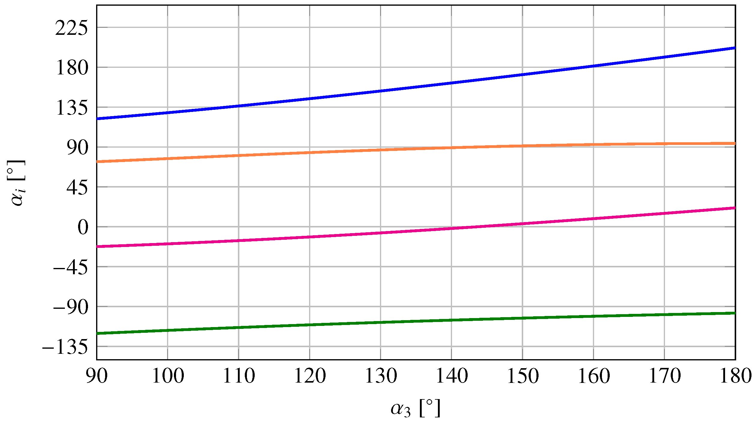
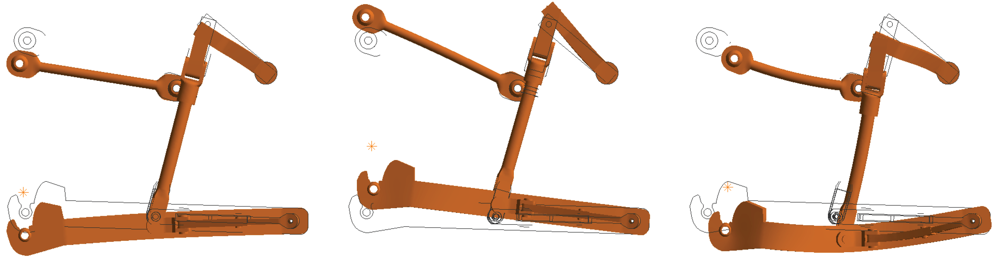
Since the three-points linkage is a 1 DoF mechanism, its configuration is defined by a single input coordinate, i.e., the angular position of the input cranks. Figure 3 shows three configurations of the linkage obtained for different angular position ${\alpha }_3$ of the input cranks, i.e., 90, 140 and 180 degrees. The angular positions ${\alpha }_i$ of all the other links can be obtained as the outcome of the position analysis of the mechanism as shown in Figure 4 for ${\alpha }_3$ varying from 90 to 180 degrees.

5. Results

For each joint, the angular positions of the connected links are used to express the compatibility condition, according to Equation (22). Furthermore, a rigid transformation is used to express constraint about the motion of the implement. All constraint equations are gathered in a overall compatibility matrix $\mathbf{B}$.

Each component of the three-points linkage is modeled using a commercial FE software and a Craig-Bampton modal reduction [13] is performed retaining only the physical connecting DoFs with other components together with an appropriate number of fixed interface modes (See

Table 2. Number of physical and modal DoFs retained for each subsystem.

Link	Physical DoFs	Modal DoFs
1 lower links	9	20
2 upper link	6	20
3 input cranks	6	20
4 lift rods	6	20
5 implement	3	0

). Therefore for each subsystem, the mass, damping and stiffness reduced order matrices are used to obtain the FRF matrix.

Finally, Equation (19) can be used to obtain the configuration-dependent FRFs, evaluated for ${\alpha }_3$ spanning the angular range 90–180 degrees with an angular step of 2 degrees.

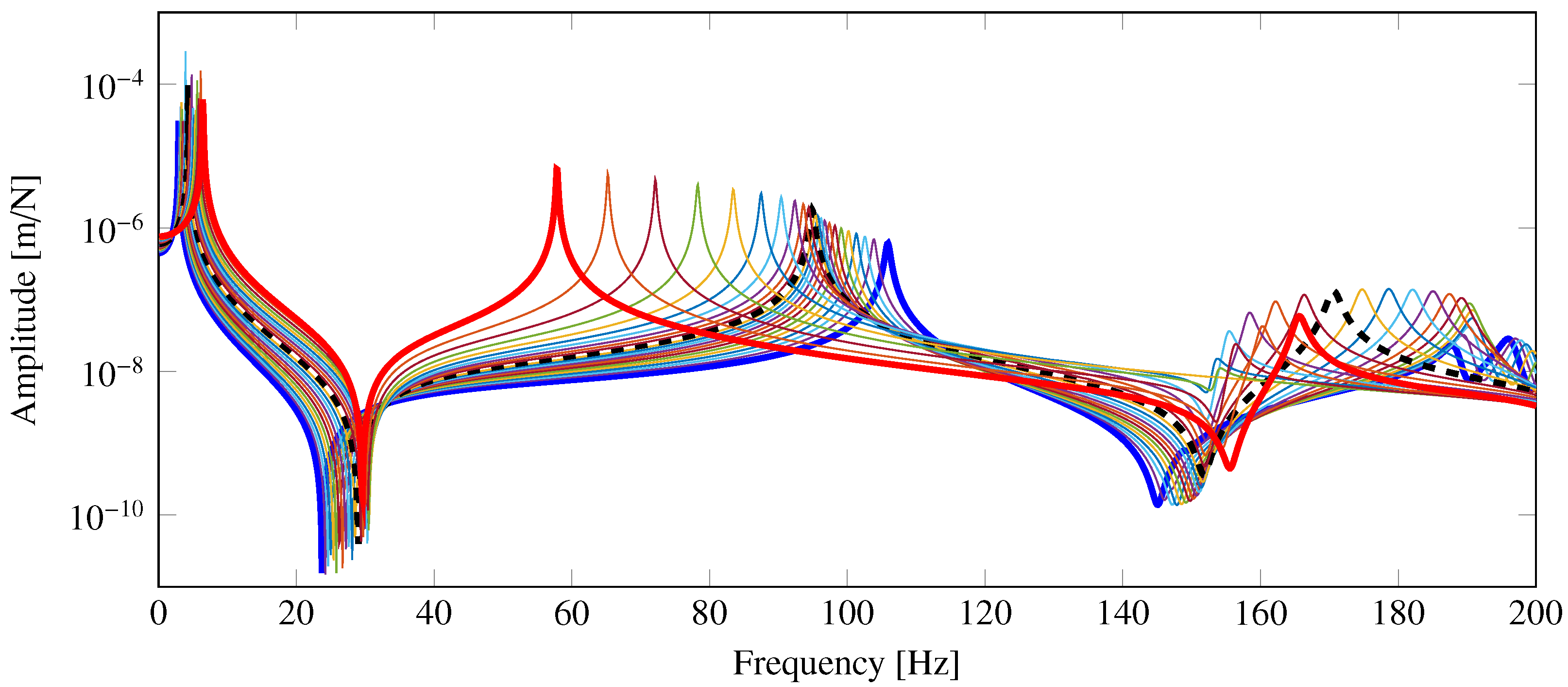
Figure 5 show the configuration-dependent drive point FRFs of the end point of the lower link (Node $E_1$) along the z direction in the frequency band 0–200 Hz. It can be noticed that the first natural frequency increases from 2.9 to 6.4 Hz, the second natural frequency decreases from 105.9 to 57.8 Hz and the third natural frequency lies in the interval from 152.8 to 191.0 Hz.

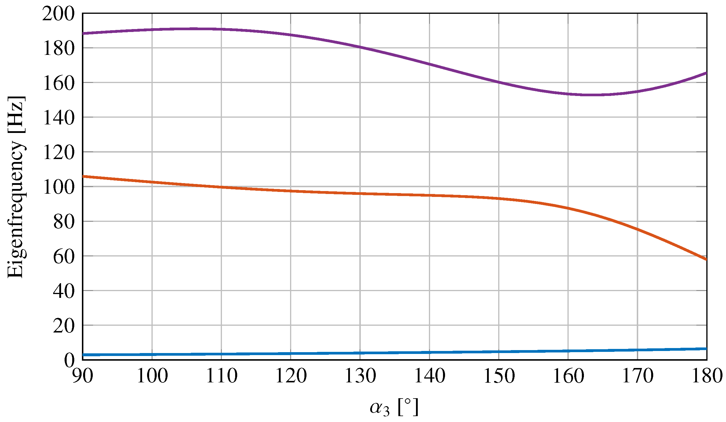
For each configuration, the first three natural frequencies and the mode shapes of the whole mechanism in the plane $XZ$ are identified. Figure 6 shows the configuration-dependent natural frequencies of the identified vibration modes of the three-point linkage.

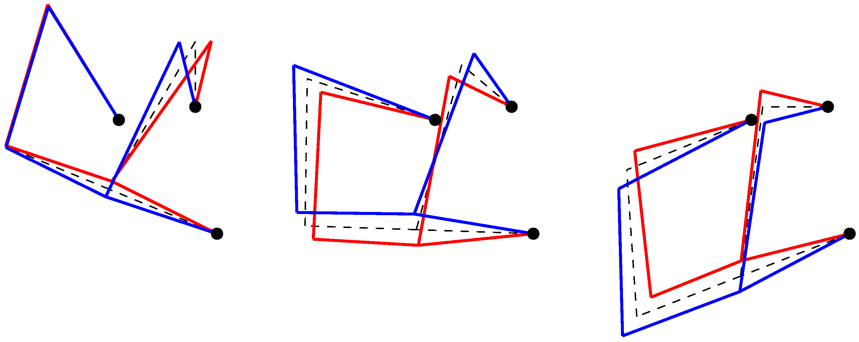
The results highlight the dependency of the natural frequencies on the configuration. Moreover, Figure 7, Figure 8 and Figure 9 show the displacements of nodes $E_1$, $E_2$, $V_1$ and $V_2$ for the first three mode shapes of the linkage in three different configurations.

Note that the nodes are joined using straight lines, so that it is not possible to observe the curvature of the different links. However, it is possible to have a quite clear idea about how the linkage oscillates.

In order to check the correctness of the procedure and the quality of the approximation due to the Craig-Bampton modal reduction of the subsystems, the assembled system in the configuration with ${\alpha }_3$ = 140${}^{\circ }$ is analyzed using a FE commercial software. The finite element model of the entire system has 250,000 nodes, and it is obtained by assembling the finite element models of the component substructures. In

Table 3. Natural frequencies.

Mode	FE [Hz]	Substructuring [Hz]
1	4.2	4.3
2	97.5	94.9
3	176.9	170.6

, the natural frequencies of modes in the plane $XZ$ below 200 Hz are compared with those obtained using the substructuring approach. The results highlight that the procedure is correctly implemented and that the approximation with 20 Craig–Bampton modes is acceptable. Figure 10 shows the mode shapes corresponding to modes 1, 2 and 3 of the assembled system in the configuration with ${\alpha }_3$ = 140${}^{\circ }$, computed using a FE commercial software. These mode shapes appear to be well correlated with those obtained using the substructuring procedure and shown in Figure 7, Figure 8 and Figure 9.

In order to quantify the computational burden of the proposed approach with respect to a more traditional approach using a commercial FE software, we calculate the computational times spent to compute a prescribed number of frequency response functions of the assembled systems in a given number of configurations and in a given frequency band with an assigned frequency step. The following parameters are used for the comparison:

• number of frequency response functions: 11;
• number of configurations: 46;
• frequency band: 0–200 Hz;
• frequency step: 0.1 Hz;

The computational time necessary to obtain the FRFs using the substructuring procedure is the sum of the following times:

• the time spent to perform the Craig-Bampton modal reduction of all subsystem with 20 fixed interface modes using a commercial FE software (226 s);
• the time spent to compute the full frequency response function matrix of the assembled system in all the considered configurations (33 s).

The computational time necessary to obtain the FRFs using a commercial FE software is the sum of the following times:

• solution of the eigenvalue problem for each of the considered configuration using 20 modes (6113 s);
• evaluation of the frequency response functions corresponding to a single excitation point (89,240 s). Note that, for every configurations, the software evaluates the frequency response functions at all the degrees of freedom.

For the considered system, the configuration-dependent substructuring approach provides frequency response functions that are 368 times faster than when using a traditional approach.

6. Conclusions

In this paper, the substructuring approach is extended to the vibrational analysis of mechanisms. The proposed approach is applied to predict the natural frequencies, the mode shapes and the frequency response functions of a three-point linkage for a set of different positions of the input link. The approach cannot be seen as an alternative to multibody system analysis but rather as a technique providing different and complementary information.

For the considered system, three frequency ranges where system resonances are possible are found; the first three mode shapes and their dependence on the configuration are shown, the frequency response functions of the system are evaluated for each configuration and the drive-point frequency response function of the end-point of the lower link is observed. This kind of result can be exploited in the preliminary design stages to highlight a possible cluster of frequencies that should be avoided as exciting frequencies or vice-versa to modify the system to move the cluster of natural frequencies of the mechanism away from the excitation frequencies.

In order to validate the effectiveness of the procedure and to quantify the computational burden, a commercial FE software is used to compute the natural frequencies, the mode shapes and the frequency response functions. The results provided by the substructuring approach are correlated with the reference results provided by the full FE model. Moreover, the computational burden required to obtain the solution using the substructuring approach is significantly lower than that using a traditional approach.

The potential applications of configuration-dependent substructuring in the dynamic analysis of a mechanism and in mechanism design are very promising.

References

- de Klerk, D.; Rixen, D.J.; Voormeeren, S. General Framework for Dynamic Substructuring: History, Review, and Classification of Techniques. AIAA J. 2008, 46, 1169–1181. [Google Scholar] [CrossRef]
- Semm, T.; Rebelein, C.; Zaeh, M. Prediction of the position dependent dynamic behavior of a machine tool considering local damping effects. CIRP J. Manuf. Sci. Technol. 2019, 27, 68–77. [Google Scholar] [CrossRef]
- Semm, T.; Nierlich, M.B.; Zaeh, M.F. Substructure Coupling of a Machine Tool in Arbitrary Axis Positions Considering Local Linear Damping Models. J. Manuf. Sci. Eng. 2019, 141, 071014. [Google Scholar] [CrossRef]
- Brunetti, J.; D’Ambrogio, W.; Fregolent, A. Dynamic coupling of substructures with sliding friction interfaces. Mech. Syst. Signal Process. 2020, 141, 106731. [Google Scholar] [CrossRef]
- Carassale, L.; Silvestri, P.; Lengu, R.; Mazzaron, P. Modeling Rail-Vehicle Coupled Dynamics by a Time-Varying Substructuring Scheme. In Dynamic Substructures, Volume 4; Linderholt, A., Allen, M.S., Mayes, R.L., Rixen, D., Eds.; Springer International Publishing: Cham, Switzerland, 2020; pp. 167–171. [Google Scholar]
- Brunetti, J.; D’Ambrogio, W.; Fregolent, A. Friction-induced vibrations in the framework of dynamic substructuring. Nonlinear Dyn. 2021, 103, 3301–3314. [Google Scholar] [CrossRef]
- Brunetti, J.; D’Ambrogio, W.; Fregolent, A. Evaluation of Different Contact Assumptions in the Analysis of Friction-Induced Vibrations Using Dynamic Substructuring. Machines 2022, 10, 384. [Google Scholar] [CrossRef]
- D’Ambrogio, W.; Fregolent, A. Experimental Dynamic Substructuring: Significance and Perspectives. In 50+ Years of AIMETA; Rega, G., Ed.; Springer International Publishing: Cham, Switzerland, 2022; pp. 305–319. [Google Scholar]
- Wittenburg, J. Dynamics of Multibody Systems, 2nd ed.; Springer: Berlin/Heidelberg, Germany, 2008. [Google Scholar]
- Shabana, A.A. Dynamics of Multibody Systems, 4th ed.; Cambridge University Press: Cambridge, UK, 2013. [Google Scholar]
- Brunetti, J.; D’Ambrogio, W.; Fregolent, A. Analysis of the Vibrations of Operators’ Seats in Agricultural Machinery Using Dynamic Substructuring. Appl. Sci. 2021, 11, 4749. [Google Scholar] [CrossRef]
- Voormeeren, S.N.; Rixen, D.J. A Family of Substructure Decoupling Techniques Based on a Dual Assembly Approach. Mech. Syst. Signal Process. 2012, 27, 379–396. [Google Scholar] [CrossRef]
- Craig, R.R., Jr.; Bampton, M. Coupling of substructures for dynamic analyses. AIAA J. 1968, 6, 1313–1319. [Google Scholar] [CrossRef] [Green Version]
Figure 1.
Two bodies r and s connected by a revolute joint in the plane orthogonal to the revolute joint axis: local ( and ) and global () reference frames.
Figure 2.
Three points linkage. (Left) 3D scheme. (Right) kinematic scheme.
Figure 3.
Three configurations of the linkage. (Left) = 90. (Middle) = 140. (Right) = 180.
Figure 4.
Angular position of the mechanism’s links. (![Machines 10 01146 i001]() ); (
); (![Machines 10 01146 i002]() ); (
); (![Machines 10 01146 i003]() ); (
); (![Machines 10 01146 i004]() ).
).
); (
); ( ); (
); ( ).
Figure 5.
Configuration dependent drive point FRF of node in the y direction. (![Machines 10 01146 i005]() ) = 90; (
) = 90; (![Machines 10 01146 i006]() ) = 180; (
) = 180; (![Machines 10 01146 i007]() ) = 140.
) = 140.
) = 90; (
) = 180; (
) = 90; () = 180; () = 140.
Figure 6.
Configuration dependent natural frequencies of vibration modes from one to three of the three-point linkage, as function of the angle of the input crank. First natural frequency (![Machines 10 01146 i008]() ); Second natural frequency (
); Second natural frequency (![Machines 10 01146 i009]() ); Third natural frequency (
); Third natural frequency (![Machines 10 01146 i010]() ).
); Second natural frequency (
); Third natural frequency (
); Second natural frequency (); Third natural frequency ().
Figure 7.
Mode 1 in three different configurations. (Left) = 90. (Middle) = 140. (Right) = 180. (![Machines 10 01146 i011]() ) Undeformed model; (
) Undeformed model; (![Machines 10 01146 i012]() ) and (
) and (![Machines 10 01146 i013]() ) extreme deformed configurations during oscillation.
) extreme deformed configurations during oscillation.
) Undeformed model; (
) and (
) Undeformed model; () and () extreme deformed configurations during oscillation.
Figure 8.
Mode 2 in three different configurations. (Left) = 90. (Middle) = 140. (Right) = 180. (![Machines 10 01146 i014]() ) Undeformed model; (
) Undeformed model; (![Machines 10 01146 i015]() ) and (
) and (![Machines 10 01146 i016]() ) extreme deformed configurations during oscillation.
Figure 9.
Mode 3 in three different configurations. (Left) = 90. (Middle) = 140. (Right) = 180. (![Machines 10 01146 i017]() ) Undeformed model; (
) Undeformed model; (![Machines 10 01146 i018]() ) and (
) and (![Machines 10 01146 i019]() ) extreme deformed configurations during oscillation.
Figure 10.
From left to right, mode shapes of the modes 1, 2 and 3 of the assembled system in the configuration with = 140, computed using a FE commercial software.