Article

Lyapunov Functions to Caputo Fractional Neural Networks with Time-Varying Delays

1
Department of Mathematics, Texas A&M University-Kingsville, Kingsville, TX 78363, USA
2
Florida Institute of Technology, Melbourne, FL 32901, USA
3
Department of Applied Mathematics, University of Plovdiv Paisii Hilendarski, 4000 Plovdiv, Bulgaria
4
School of Mathematics, Statistics and Applied Mathematics, National University of Ireland, H91 CF50 Galway, Ireland
*
Author to whom correspondence should be addressed.
Distinguished University Professor of Mathematics.
Axioms 2018, 7(2), 30; https://doi.org/10.3390/axioms7020030
Submission received: 29 March 2018 / Revised: 3 May 2018 / Accepted: 5 May 2018 / Published: 9 May 2018
(This article belongs to the Special Issue Fractional Differential Equations)

Abstract

:
One of the main properties of solutions of nonlinear Caputo fractional neural networks is stability and often the direct Lyapunov method is used to study stability properties (usually these Lyapunov functions do not depend on the time variable). In connection with the Lyapunov fractional method we present a brief overview of the most popular fractional order derivatives of Lyapunov functions among Caputo fractional delay differential equations. These derivatives are applied to various types of neural networks with variable coefficients and time-varying delays. We show that quadratic Lyapunov functions and their Caputo fractional derivatives are not applicable in some cases when one studies stability properties. Some sufficient conditions for stability of equilibrium of nonlinear Caputo fractional neural networks with time dependent transmission delays, time varying self-regulating parameters of all units and time varying functions of the connection between two neurons in the network are obtained. The cases of time varying Lipschitz coefficients as well as nonLipschitz activation functions are studied. We illustrate our theory on particular nonlinear Caputo fractional neural networks.

1. Introduction

Neural networks have a wide range of applications in pattern recognition, associative memory, combinatorial optimization, etc. Delays are incorporated into the model equations of the networks because of the finite speeds of the switching and transmission of signals in a network and this leads to time delays in a working network. It was observed both experimentally and numerically in [1] that time delay could induce instability, causing sustained oscillations which may be harmful to a system. Additionally, when one considers memory and hereditary properties of various materials and processes ([2]), it is natural to consider fractional derivatives in the model. Neural networks in biology, coupled lasers, wireless communication and power-grid networks in physics and engineering ([3,4,5,6]) are modeled by fractional order differential equations.
In controlling nonlinear systems, the Lyapunov second method provides a way to analyze the stability of the system without explicitly solving the differential equations. Stability results concerning integer-order neural networks can be found in [7,8,9] and recently Lyapunov stability theory for fractional order systems was discussed (see [10,11]). Fractional order Lyapunov stability theory was applied for various types of fractional neural networks using quadratic Lyapunov functions (see [2,12,13,14]) and stability analysis of fractional-order delay neural networks can be found in [15,16,17,18,19], for example. Finite-time stability of fractional-order neural networks with constant transmission delay and constant self-regulating parameters is studied in [20,21] and for distributed delays and constant self-regulating parameters see [22].
The main goal of this paper is to study stability properties of Caputo fractional order neural networks with delays. We study the general case of time varying transmission delays as well as time varying self-regulating parameters of all units and time varying functions of the connection between two neurons in the network. Note that usually in the literature the activation functions in the models are Lipschitz with constant Lipschitz coefficients. In this paper, the cases of time varying Lipschitz coefficients as well as nonLipschitz activation functions are studied. The investigation is based on the fractional Lyapunov method. It is worth pointing out that the Lyapunov functional method can not be easily generalized to fractional order systems. It is mainly connected with the derivative taken in the given fractional system. Taking these factors into consideration, we present a brief overview of the existing literature on the various definitions of fractional order derivatives of Lyapunov functions among Caputo fractional differential equations with variable delays and we compare them in several examples, discussing their advantages and disadvantages. Using the appropriate fractional derivative of Lyapunov functions, some stability sufficient criteria are provided and illustrated with examples.

2. Lyapunov Functions and Their Derivatives among the Delay Fractional Differential Equation

We first consider the derivative of Lyapunov functions among the delay fractional differential equation.
In this paper we consider Caputo fractional derivatives with order q ( 0 , 1 ) defined by (see, for example [23])
t 0 C D t q m ( t ) = 1 Γ 1 q t 0 t t s q m ( s ) d s , t t 0 ,
where Γ ( . ) denotes the Gamma function.
Consider the initial value problem (IVP) for the nonlinear Caputo fractional delay differential equations (FrDDE)
t 0 C D t q x ( t ) = f ( t , x t ) for t [ t 0 , t 0 + T ) , x ( t 0 + Θ ) = ψ 0 ( Θ ) , Θ [ r , 0 ] ,
where x R n , f C [ [ t 0 , t 0 + T ) × R n , R n ] , t 0 R + is the initial time, ψ 0 C ( [ r , 0 ] , R n ) is the initial function, T and for any t [ t 0 , t 0 + T ) the notation x t ( Θ ) = x ( t + Θ ) , Θ [ r , 0 ] is used.
Let x ( t ) , t [ t 0 r , t 0 + T ) , be a solution of the IVP for the FrDDE (1) and let V ( t , x ) be a Lyapunov function, i.e., V ( t , x ) : [ t 0 r , t 0 + T ) × Δ R + is continuous and locally Lipschitzian with respect to its second argument, where Δ R n , 0 Δ .
In the literature there are three types of derivatives of Lyapunov functions among solutions of fractional differential equations used to study stability properties:
-
first type–Let x ( t ) be a solution of IVP for FrDDE (1). Then the Caputo fractional derivative of the Lyapunov function V ( t , x ( t ) ) is defined by
t 0 C D t q V ( t , x ( t ) ) = 1 Γ 1 q t 0 t t s q d d s V ( s , x ( s ) ) d s , t ( t 0 , t 0 + T ) .
This type of derivative is applicable for continuously differentiable Lyapunov functions. It is used mainly for quadratic Lyapunov functions to study several stability properties of fractional differential equations (see, for example [10]).
-
second type–this type of derivative of V ( t , x ) among FrDDE (1) was introduced by I. Stamova, G. Stamov (Definition 1.12 [24]):
D ( 1 ) + V ( t , ϕ ( 0 ) ) = lim sup h 0 1 h q V ( t , ϕ ( 0 ) ) V ( t h , x h q f ( t , ϕ 0 ) ) , t ( t 0 , t 0 + T )
where ϕ C ( [ r , 0 ] , R n ) and the notation ϕ 0 ( Θ ) = ϕ ( 0 + Θ ) , Θ [ r , 0 ] is used.
Note that the operator defined by (3) has no memory (the memory is typical for fractional derivatives) (see Case 2.1 of Example 1 and Case 2.2 of Example 2).
Remark 1.
In general D ( 1 ) + V ( t , x ( t ) ) 0 C D t q V ( t , x ( t ) ) where x ( t ) is a solution of (1).
Now, let us recall the remark in [25] concerning definition (3) where V ( t h , x h q f ( t , x ) ) is defined by
V ( t h , x h q f ( t , x ) ) = r = 1 [ t t 0 h ] ( 1 ) r + 1 q C r V ( t r h , x h q f ( t , x ) )
where q C r = q ( q 1 ) ( q r + 1 ) r ! .
Following this notation the fractional derivative of the Lyapunov function is defined by
D ( 1 ) + V ( t , ϕ ( 0 ) ; t 0 ) = lim sup h 0 1 h q V ( t , ϕ ( 0 ) ) r = 1 [ t t 0 h ] ( 1 ) r + 1 q C r V ( t r h , ϕ ( 0 ) h q f ( t , ϕ 0 ) ) .
The derivative (4) has memory and it depends on the initial time t 0 . It is closer to both the Grunwald-Letnikov fractional derivative and the Riemann-Liouville fractional derivative, than to the Caputo fractional derivative of a function. We will call the derivative (4) the Dini fractional derivative of the Lyapunov function. The Dini fractional derivative is applicable for continuous Lyapunov functions.
Remark 2.
In the general case D ( 1 ) + V ( t , ϕ ( 0 ) ) D ( 1 ) + V ( t , ϕ ( 0 ) ) .
-
third type–for any ϕ C ( [ r , 0 ] , R n ) the derivative of the Lyapunov function V ( t , x ) among IVP for FrDDE (1) with initial point t 0 and initial function ψ 0 C ( [ r , 0 ] , R n ) is defined by:
( 1 ) c D + q V ( t , ϕ ( 0 ) ; t 0 , ψ 0 ) = lim sup h 0 + 1 h q { V ( t , ϕ ( 0 ) ) V ( t 0 , ψ 0 ( 0 ) ) r = 1 [ t t 0 h ] ( 1 ) r + 1 q C r V ( t r h , ϕ ( 0 ) h q f ( t , ϕ 0 ) ) V ( t 0 , ψ 0 ( 0 ) ) } for t ( t 0 , t 0 + T ) ,
or its equivalent
( 1 ) c D + q V ( t , ϕ ( 0 ) ; t 0 , ψ 0 ) = lim sup h 0 + 1 h q V ( t , ϕ ( 0 ) ) + r = 1 [ t t 0 h ] ( 1 ) r q C r V ( t r h , ϕ ( 0 ) h q f ( t , ϕ 0 ) ) V ( t 0 , ψ 0 ( 0 ) ) ( t t 0 ) q Γ ( 1 q ) , for t ( t 0 , t 0 + T ) .
The derivative (6) depends significantly on both the fractional order q and the initial data ( t 0 , ψ 0 ) of IVP for FrDDE (1) and this type of derivative is close to the idea of the Caputo fractional derivative of a function.
We call the derivative given by (5) or its equivalent (6) the Caputo fractional Dini derivative. This type of derivative is applicable for continuous Lyapunov functions (see, for example [26,27,28]).
Remark 3.
The equality
( 1 ) c D + q V ( t , ϕ ( 0 ) ; t 0 , ψ 0 ) = D ( 1 ) + V ( t , ϕ ( 0 ) ; t 0 ) V ( t 0 , ψ 0 ( 0 ) ) ( t t 0 ) q Γ ( 1 q )
holds for any t ( t 0 , t 0 + T ) , ϕ 0 C ( [ r , 0 ] , R n ) and for any initial data ( t 0 , ψ 0 ) R + × C ( [ r , 0 ] , R n ) :
( 1 ) c D + q V ( t , ϕ ( 0 ) ; t 0 , ψ 0 ) = D ( 1 ) + V ( t , ϕ ( 0 ) ; t 0 ) , i f V ( t 0 , ψ 0 ( 0 ) ) = 0
( 1 ) c D + q V ( t , ϕ ( 0 ) ; t 0 , ψ 0 ) < D ( 1 ) + V ( t , ϕ ( 0 ) ; t 0 ) , i f V ( t 0 , ψ 0 ( 0 ) ) > 0 .
Remark 4.
Note that in the case of delays in the differential equations, the derivative of the Lyapunov function is considered for functions ϕ C ( [ r , 0 ] , R n ) and points t such that V ( t , ϕ ( 0 ) ) = sup s [ r , 0 ] V ( t + s , ϕ ( s ) ) . This condition is called the Razumikhin condition.
We will illustrate the application of the above given derivatives on the quadratic Lyapunov function (used in stability of neural networks [2,12,13,14]).
Example 1.
Let n = 1 . Consider the quadratic Lyapunov function i.e., V ( t , x ) = x 2 .
Case 1. First type of derivative. Let x ( t ) be a solution of the IVP for FrDDE (1). According to [29] we get
t 0 C D t q V ( t , x ( t ) ) = 2 Γ 1 q t 0 t t s q x ( s ) x ( s ) d s 2 x ( t ) t 0 C D t q x ( t ) = 2 x ( t ) f ( t , x t ) .
Case 2. Second type of derivative.
Case 2.1: Let the function ϕ C ( [ r , 0 ] , R n ) . From Formula (3) we obtain
D ( 1 ) + V ( t , ϕ ( 0 ) ) = lim sup h 0 1 h q ϕ ( 0 ) 2 ϕ ( 0 ) h q f ( t , ϕ 0 ) 2 = 2 ϕ ( 0 ) f ( t , ϕ 0 ) .
It is seen that the derivative D ( 1 ) + V ( t , ϕ ( 0 ) ) does not depend on any initial data of the fractional equation.
Case 2.2: Dini fractional derivative. Let the function ϕ C ( [ r , 0 ] , R n ) . From Formula (4) we obtain
D ( 1 ) + V ( t , ϕ ( 0 ) ; t 0 ) = lim sup h 0 1 h q ϕ ( 0 ) 2 r = 1 [ t t 0 h ] ( 1 ) r + 1 q C r ϕ ( 0 ) h q f ( t , ϕ 0 ) 2 = lim sup h 0 1 h q ϕ ( 0 ) 2 + r = 1 [ t t 0 h ] ( 1 ) r q C r ϕ ( 0 ) h q f ( t , ϕ 0 ) 2 = ϕ ( 0 ) 2 lim sup h 0 1 h q r = 0 [ t t 0 h ] ( 1 ) r q C r + lim sup h 0 2 ϕ ( 0 ) f ( t , ϕ 0 ) + h q f 2 ( t , ϕ 0 ) r = 1 [ t t 0 h ] ( 1 ) r q C r ] = 2 ϕ ( 0 ) f ( t , ϕ 0 ) + ϕ ( 0 ) 2 ( t t 0 ) q Γ ( 1 q )
The Dini fractional derivative depends on both the fractional order q and initial time.
Case 3. Third type of derivative. Caputo fractional Dini derivative. According to Remark 4 and Case 2.2 the inequality
( 1 ) c D + q V ( t , ϕ ( 0 ) ; 0 , ψ 0 ) = 2 ϕ ( 0 ) f ( t , ϕ 0 ) + ϕ ( 0 ) 2 ( t t 0 ) q Γ ( 1 q ) ψ 0 ( 0 ) 2 ( t t 0 ) q Γ ( 1 q )
holds.
The Caputo fractional Dini derivative depends on both the fractional order q and initial data ( t 0 , ψ 0 ) .
From the literature we note that one of the sufficient conditions for stability is connected with the sign of the derivative of the Lyapunov function of the equation.
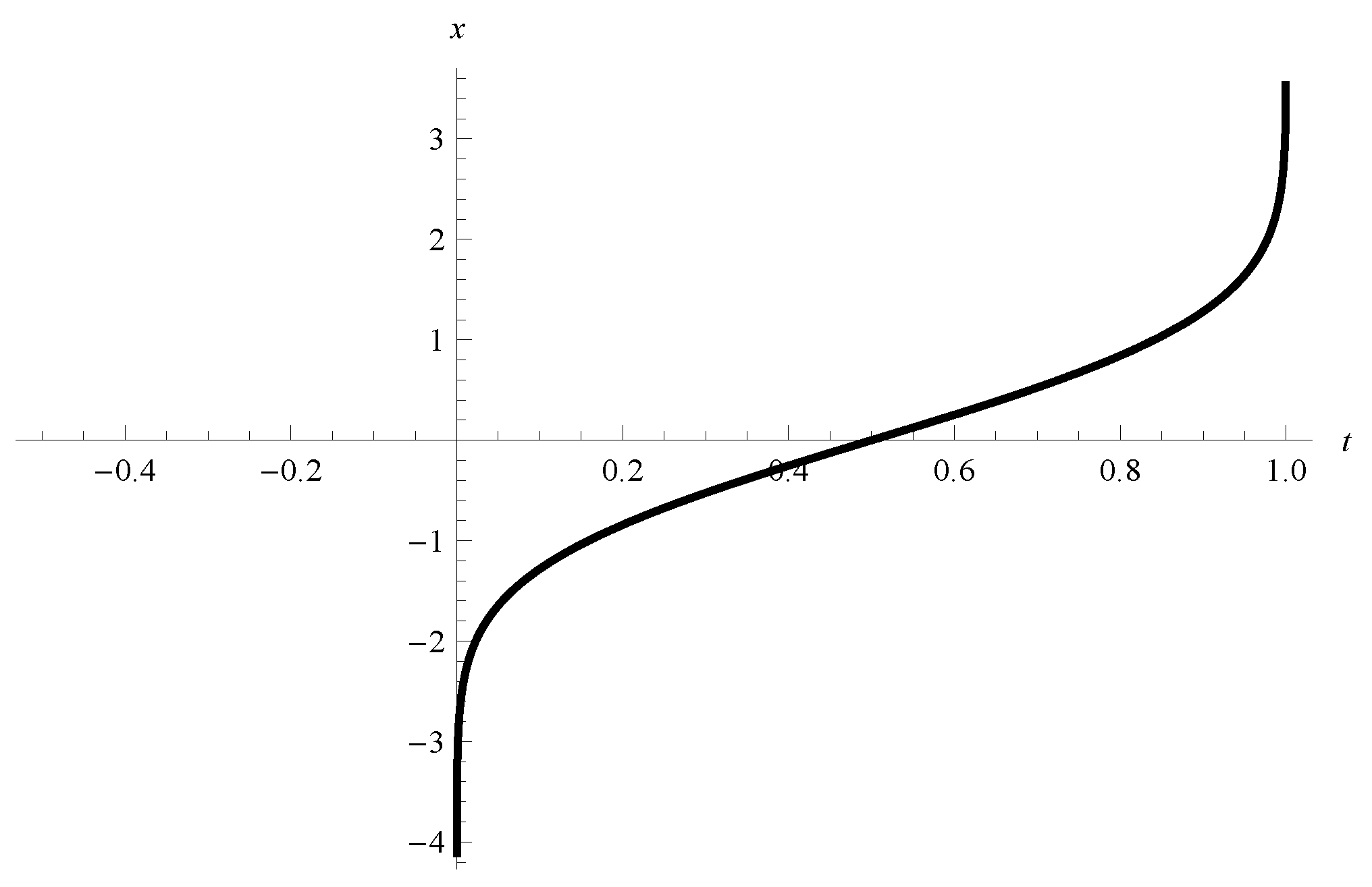
Example 2.
Consider the IVP for the scalar linear FrDDE
0 C D t q x ( t ) = g ( t ) x ( t ) + 0.1 x ( t π ) f o r t > 0 , x ( s ) = 1 f o r s [ π , 0 ] ,
where q ( 0 , 1 ) , g ( t ) = 0.5 0 R L D q sin 2 ( t ) + 0.1 s i n 2 ( t ) + 0.1 0.1 , t > 0 .
Case 1. Consider the quadratic Lyapunov function [12,13,14]) i.e., V ( t , x ) = x 2 . Let x ( t ) be a solution of IVP for FrDDE (14) and t > 0 be such that V ( t , x ( t ) ) = x 2 ( t ) = sup s [ π , t ] x 2 ( s ) = sup s [ π , t ] V ( s , x ( s ) ) . Then according to [29] we get
0 C D t q V ( t , x ( t ) ) 2 x ( t ) 0 C D t q x ( t ) = 2 ( x ( t ) ) 2 g ( t ) + 0.2 x ( t ) x ( t π ) 2 x 2 ( t ) ( 0.1 + g ( t ) ) .
The sign of 0 C D t q V ( t , x ( t ) ) is changeable (the graph of the function g ( t ) + 0.1 for various values of q is given on Figure 1).
Case 2. Consider the function V ( t , x ) = ( sin 2 ( t ) + 0.1 ) x 2 .
Case 2.1: Caputo fractional derivative. Let x ( t ) be a solution of IVP for FrDDE (14). From Equation (2) we obtain
0 C D t q V ( t , x ( t ) ) = 1 Γ 1 q 0 t t s q 2 ( sin 2 ( s ) + 0.1 ) x ( s ) x ( s ) + sin ( 2 s ) x 2 ( s ) d s .
The fractional derivative of this function V is difficult to obtain so it is difficult to discuss its sign.
Case 2.2: Use Formula (3) and for any function ϕ C ( [ π , 0 ] , R ) and any point t > 0 such that V ( t , ϕ ( 0 ) ) = ( sin 2 ( t ) + 0.1 ) ϕ 2 ( 0 ) = sup s [ π , 0 ] ( sin 2 ( t + s ) + 0.1 ) ϕ 2 ( s ) = sup s [ π , 0 ] V ( t + s , ϕ ( s ) ) we obtain
D ( 14 ) + V ( t , ϕ ( 0 ) ) = lim sup h 0 1 h q [ sin 2 ( t ) sin 2 ( t h ) ϕ 2 ( 0 ) 2 h q ( sin 2 ( t h ) + 0.1 ) ϕ ( 0 ) ϕ ( 0 ) g ( t ) + 0.1 ϕ ( 1 ) + h 2 q ( sin 2 ( t h ) + 0.1 ) ϕ ( 0 ) g ( t ) + 0.1 ϕ ( π ) 2 ] = 2 ϕ ( 0 ) ( s i n 2 ( t ) + 0.1 ) ( ϕ ( 0 ) g ( t ) + 0.1 ϕ ( π ) ) 2 ϕ 2 ( 0 ) ( s i n 2 ( t ) + 0.1 ) g ( t ) + 0.2 ϕ ( 0 ) ϕ ( π ) ( s i n 2 ( t ) + 0.1 ) 2 ϕ 2 ( 0 ) ( s i n 2 ( t ) + 0.1 ) g ( t ) + 0.1 ϕ 2 ( 0 ) ( s i n 2 ( t ) + 0.1 ) + 0.1 ϕ 2 ( π ) ( s i n 2 ( t π ) + 0.1 ) 2 ϕ 2 ( 0 ) ( s i n 2 ( t ) + 0.1 ) ( g ( t ) + 0.1 )
i.e., the sign of the derivative D ( 14 ) + V ( t , ϕ ) is changeable.
Case 2.3: Dini fractional derivative. For any function ϕ C ( [ π , 0 ] , R ) and t > 0 such that V ( t , ϕ ( 0 ) ) = ( sin 2 ( t ) + 0.1 ) ϕ 2 ( 0 ) = sup s [ π , 0 ] ( sin 2 ( t + s ) + 0.1 ) ϕ 2 ( s ) = sup s [ π , 0 ] V ( t + s , ϕ ( s ) ) we apply Formula (4) and obtain
D ( 14 ) + V ( t , ϕ ( 0 ) ; 0 ) = lim sup h 0 1 h q [ ( sin 2 ( t ) + 0.1 ) ϕ 2 ( 0 ) r = 1 [ t h ] ( 1 ) r + 1 q C r ( sin 2 ( t r h ) + 0.1 ) ϕ ( 0 ) h q ϕ ( 0 ) g ( t ) + 0.1 ϕ ( π ) 2 ] = ϕ 2 ( 0 ) lim sup h 0 1 h q r = 1 [ t h ] ( 1 ) r ( sin 2 ( t r h ) + 0.1 ) 2 lim sup h 0 r = 1 [ t h ] ( 1 ) r q C r ( sin 2 ( t r h ) + 0.1 ) ϕ 2 ( 0 ) g ( t ) + 0.1 ϕ ( 0 ) ϕ ( π ) + lim sup h 0 h q r = 1 [ t h ] ( 1 ) r + 1 q C r ( sin 2 ( t r h ) + 0.1 ) ϕ ( 0 ) g ( t ) + 0.1 ϕ ( π ) 2 2 ϕ 2 ( 0 ) ( g ( t ) + 0.1 ) ( sin 2 ( t ) + 0.1 ) + ϕ 2 ( 0 ) 0 R L D q sin 2 ( t ) + 0.1 = 0 .
Case 2.4: Caputo fractional Dini derivative. According to Remark 4 and Case 2.3 the inequality
( 14 ) c D + q V ( t , ϕ ( 0 ) ; 0 , ψ 0 ) = D ( 14 ) + V ( t , ϕ ( 0 ) ; 0 ) 0.1 ψ 0 2 ( 0 ) t q Γ ( 1 q ) = 0.1 ψ 0 2 ( 0 ) t q Γ ( 1 q ) 0
holds.
Therefore, for (14) both the Dini fractional derivative and the Caputo fractional Dini derivative seem to be more applicable than the Caputo fractional derivative of Lyapunov function.
Remark 5.
The above example notes that the quadratic function for studying stability properties of neural network might not be successful (especially when the right hand side depends directly on the time variable). Formula (3) is not appropriate for applications to fractional equations. The most general derivatives for non-homogenous fractional differential equations are Dini fractional derivatives and Caputo fractional Dini derivatives.

3. Remarks on Some Applications of Derivatives of Lyapunov Functions

Some authors use the derivative defined by (3) to study stability properties of delay fractional differential equations ([24,30]) and delayed reaction-diffusion cellular neural networks of fractional order ([31]). The proofs are based on the following result:
Lemma 1.
([24]) Assume that:
1.
The function g : [ t 0 , ) × R + R is continuous in [ t 0 , ) × R + and is nondecreasing in u for each t t 0 .
2.
The maximal solution u + ( t ) of the IVP for scalar Caputo fractional differential equation t 0 c D t q u ( t ) = g ( t , u ( t ) ) , t > t 0 , u ( t 0 ) = 1 exists on [ t 0 , ) .
3.
The Lipschitz function V ( t , x ) is such that for t t 0 , ϕ C ( [ r , 0 ] , Δ ) the inequality
D ( 1 ) + V ( t , ϕ ( 0 ) ) g ( t ; V ( t , ϕ ( 0 ) ) )
is valid whenever V ( t + Θ , ϕ ( Θ ) ) V ( t , ϕ ( 0 ) ) for r Θ 0 where Δ R n , 0 Δ .
Then max r Θ 0 V ( t 0 + Θ ) u 0 implies V ( t , x ( t ; t 0 , ϕ 0 ) ) u + ( t ; t 0 , u 0 ) , t [ t 0 , ) , where x ( t ; t 0 , ϕ 0 ) is the solution of (1) with initial data ( t 0 , ψ 0 ) R + × C [ [ r , 0 ] , Δ ] .
The claim of Lemma 1 is not true. We will give a counterexample.
Example 3.
Consider the IVP for FrDDE (1) with n = 1 , t 0 = 0 , r = 0 , g ( t , u ) = h ( t ) , f ( t , x t ) = 0.5 h ( t ) x ( t ) , ψ 0 ( t ) 1 , and h ( t ) = t 2 q p F q [ { 1 } , { 3 / 2 q / 2 , 2 q / 2 } , ( t 2 / 4 ) ] Γ ( 1 q ) ( 1 q ) ( 2 q ) where p F q [ { a } , { b , c } , z ] = n = 0 ( a ) n ( b ) n ( c ) n z n n ! with ( a ) n = a ( a + 1 ) ( a + 2 ) ( a + n 1 ) is the general hypergeometric function or Aomoto-Gelfand hypergeometric function [32]. We denote its solution by x ( t ) .
Consider the Lyapunov function V ( t , x ) = x 2 . According to Example 1, Case 2.1, Equation (11) we get D ( 1 ) + V ( t , ϕ ( 0 ) ) = 2 ϕ ( 0 ) f ( t , ϕ 0 ) = h ( t ) .
The function u ( t ) = c o s ( t ) is a solution of the IVP for the comparison scalar fractional differential equation
0 c D t q u ( t ) = h ( t ) , t > 0 , u ( 0 ) = 1
Then V ( 0 , x ( 0 ) ) = 1 but the inequality
0 V ( t , x ( t ) ) = ( x ( t ) ) 2 cos ( t ) = u ( t )
does not hold for t 0 .
The application of the derivative D ( 1 ) + V ( t , ϕ ( 0 ) ) defined by (3) is not appropriate in studying stability properties of neural networks of fractional order (as presented in [31]). We will consider fractional neural networks with delays and using Lyapunov functions and their Caputo fractional derivative, Dini fractional derivative or Caputo fractional Dini derivative (and without applying Lemma 1) we study stability.

4. Stability for Caputo Fractional Order Neural Networks with Time Varying Delays

4.1. System Description

Consider the general model of fractional order neural networks with time varying delay (FODNN)
0 C D t q x i ( t ) = c i ( t ) x i ( t ) + j = 1 n a i j ( t ) f j ( x j ( t ) ) + j = 1 n b i j ( t ) g j ( x j ( t τ ( t ) ) ) + I i ( t ) for t > 0 , i = 1 , 2 , n ,
where q ( 0 , 1 ) , n represents the number of units in the network, x i ( t ) is the pseudostate variable of the i-th unit of master system, x ( t ) = [ x 1 ( t ) , x 2 ( t ) , , x n ( t ) ] T R n , c i ( t ) > 0 , i = 1 , 2 , , n , is the self-regulating parameters of the i-th unit, , a i j ( t ) , b i j ( t ) , i , j = 1 , 2 , , n , correspond to the connection of the i-th neuron to the j-th neuron at times t and t τ ( t ) respectively, f j ( x j ( t ) ) and g j ( x j ( t τ ( t ) ) ) denote the activation functions of the neurons at time t and t τ ( t ) , respectively, f ( x ) = [ f 1 ( x 1 ) , f 2 ( x 2 ) , , f n ( x n ) ] T , g ( x ) = [ g 1 ( x 1 ) , g 2 ( x 2 ) , , g n ( x n ) ] T and I = [ I 1 , I 2 , , I n ] T is an external bias vector, τ ( t ) C ( R + , [ 0 , r ] ) is the transmission delay.
The initial conditions of the given system (15) are listed as
x i ( t ) = ψ i ( t ) for t [ r , 0 ] ,
where ψ i C ( r , 0 ] , R ) , i = 1 , 2 , , n , with the norm | | ψ | | = sup t [ r , 0 ] i = 1 n | ψ i ( t ) | .
Remark 6.
The problem of existence and uniqueness of equilibrium states of fractional-order neural networks was investigated by several authors; for sufficient conditions which guarantee the existence and uniqueness of solutions for FODNN with constant delays we refer the reader to [15].
Definition 1.
A vector x * R n , x * = ( x 1 * , x 2 * , , x n * ) is an equilibrium point of Caputo FODNN (15), if the equalities 0 = c i ( t ) x i * + j = 1 n a i j ( t ) f j ( x j * ) + j = 1 n b i j ( t ) g j ( x j * ) + I i ( t ) hold for all t > 0 , i = 1 , 2 , , n .
We will discuss the equilibrium points on some FODNN with various activation functions. It will be useful for stability analysis.
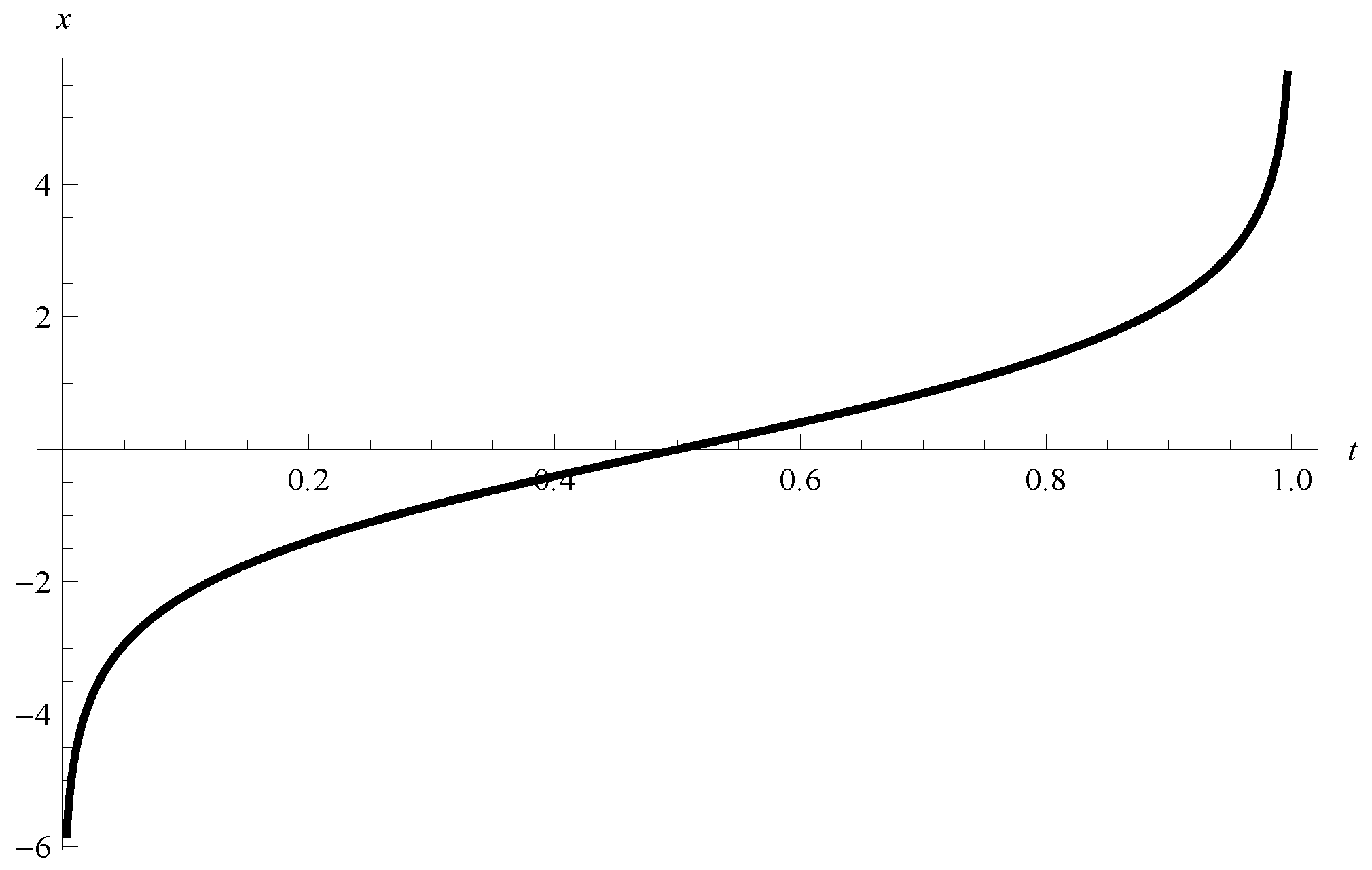
Example 4.
Consider the system of FODNN (15) with n = 3 , c i ( t ) c i , with the activation functions f j ( s ) = g j ( s ) = 0.5 t a n h ( s ) , and a i j ( t ) a i j , b i j ( t ) b i j and I i ( t ) I i . Then the point x * = ( ξ 1 , ξ 2 , ξ 3 ) is an equilibrium point iff 0 = 2 c i ξ i + j = 1 3 a i , j t a n h ( ξ i ) + j = 1 3 b i , j t a n h ( ξ i ) + I i , i = 1 , 2 , 3 .
Example 5.
Let n = 1 , c is a constant and consider the scalar FODNN
0 C D t q x ( t ) = c x ( t ) + a ( t ) f ( x ( t ) ) + b ( t ) g ( x ( t r ) ) + I f o r t > 0 .
Case 1. Let I = 0.5 π c and the activation function be the cosine function f ( u ) = g ( u ) = cos ( u ) (see [33]).
The point x * = 0.5 π is an equilibrium point of FODNN(17) because c 0.5 π + a ( t ) cos ( 0.5 π ) + a ( t ) cos ( 0.5 π ) + 0.5 π c = 0 for all t > 0 .
Case 2. Let I = 0.5 c and the activation function be the Probit function f ( u ) = g ( u ) = 2 e r f 1 ( 2 u 1 ) (see Figure 2) where e r f ( u ) = 2 π 0 u e t 2 d t is the error function. Then e r f 1 ( 0 ) = 0 .
The point x * = 0.5 is an equilibrium point of FODNN(17) because c 0.5 + a ( t ) f ( 0.5 ) + b ( t ) g ( 0.5 ) + 0.5 c = 0 for all t > 0 .
Case 3. Let I = 0.5 c and the activation function be the Logit function f ( u ) = g ( u ) = log u 1 u (see Figure 3). Then f ( 0.5 ) = 0 .
The point x * = 0.5 is an equilibrium point of Caputo FODNN (17) because c 0.5 + a ( t ) f ( 0.5 ) + b ( t ) g ( 0.5 ) + 0.5 c = 0 for all t > 0 .
Assumption 1.
Let the Caputo FODNN (15) have an equilibrium point x * .
If Assumption 1 is satisfied then we can shift the equilibrium point x * of system (15) to the origin. The transformation y ( t ) = x ( t ) x * is used to put system (15) in the following form:
0 C D t q y i ( t ) = c i ( t ) y i ( t ) + j = 1 n a i j ( t ) F j ( y j ( t ) ) + j = 1 n b i j ( t ) G j ( y j ( t τ ( t ) ) ) for t > 0 , i = 1 , 2 , n ,
where F j ( u ) = f j ( u + x j * ) f j ( x j * ) , G j ( u ) = g j ( u + x j * ) g j ( x j * ) , u R , j = 1 , 2 , , n .
We will give the Dini fractional derivative of a Lyapunov function depending directly on the time t among the FODNN (18) which will be used in the proofs of some of the main results.
Example 6.
Consider the IVP for FODNN (18).
Consider the function V ( t , x ) = p ( t ) i = 1 n x i 2 where p C ( [ r , ) , R + : α p ( t ) β for t r where α , β > 0 are constants. Let ϕ C ( [ r , 0 ] , R n ) and t > 0 be such that V ( t , ϕ ( 0 ) ) = p ( t ) i = 1 n ϕ i 2 ( 0 ) = sup s [ r , 0 ] p ( t + s ) i = 1 n ϕ i 2 ( s ) = sup s [ r , 0 ] V ( t + s , ϕ ( s ) ) . Then from Formula (4) we obtain for the Dini fractional derivative:
D ( 18 ) + V ( t , ϕ ( 0 ) ; 0 ) = i = 1 n ϕ i 2 ( 0 ) lim sup h 0 1 h q r = 1 [ t h ] ( 1 ) r p ( t r h ) + 2 i = 1 n c i ( t ) ϕ i 2 ( 0 ) lim sup h 0 r = 1 [ t h ] ( 1 ) r q C r p ( t r h ) 2 i = 1 n ϕ i ( 0 ) j = 1 n a i j ( t ) F j ( ϕ j ( 0 ) ) lim sup h 0 r = 1 [ t h ] ( 1 ) r q C r p ( t r h ) 2 i = 1 n ϕ i ( 0 ) j = 1 n b i j ( t ) G j ( ϕ j ( τ ( t ) ) lim sup h 0 r = 1 [ t h ] ( 1 ) r q C r p ( t r h ) + lim sup h 0 h q r = 1 [ t h ] ( 1 ) r + 1 q C r p ( t r h ) i = 1 n ( c i ( t ) ϕ i ( 0 ) + j = 1 n a i j ( t ) F j ( ϕ j ( 0 ) ) ) + j = 1 n b i j ( t ) G j ( ϕ j ( τ ( t ) ) ) 2 2 p ( t ) i = 1 n c i ( t ) ϕ i 2 ( 0 ) + i = 1 n ϕ i ( 0 ) j = 1 n a i j ( t ) F j ( ϕ j ( 0 ) ) + b i j ( t ) G j ( ϕ j ( τ ( t ) ) + i = 1 n ϕ i 2 ( 0 ) 0 R L D q p ( t ) .

4.2. Some Results for Caputo Fractional Differential Equations

We will give some results for fractional derivatives of Lyapunov functions among Caputo fractional differential equations which will be used for our main results concerning the stability of FODNN.
Lemma 2.
([29]). Let P R n × n be constant, symmetric and positive definite matrix and X ( t ) : R + R n be a function with the Caputo fractional derivative existing.
Then 1 2 0 C D t q x T ( t ) P x ( t ) x T ( t ) P 0 C D t q x ( t ) , t 0 .
Lemma 3.
(Theorem 3.1 [16]). Let w 1 , w 2 C ( R , R + ) be nondecreasing functions, w i ( s ) > 0 , i = 1 , 2 for s > 0 , w i ( 0 ) = 0 , i = 1 , 2 , w 2 ( s ) us strictly increasing and there exists a continuously differentiable Lyapunov function V ( t , x ) R + × R n R + such that
(i) 
w 1 ( | | x | | ) V ( t , x ) w 2 ( | | x | | ) , t 0 , x R n ,
(ii) 
for any t > 0 such that sup Θ [ r , t ] V ( Θ , x ( Θ ) ) = V ( t , x ( t ) ) the inequality
0 C D t β V ( t , x ( t ) ) 0
holds where x ( t ) is a solution of (1) with t 0 = 0 .
Then the equilibrium point of (1) is uniformly stable.
For the Caputo fractional Dini derivative we have:
Lemma 4.
(Theorem 6 [34]). Assume x = 0 be an equilibrium point for (1) with T = and there exists a Lyapunov function V ( t , x ) : V ( t , 0 ) = 0 , t 0 , such that
(i) 
α 1 ( | | x | | ) V ( t , x ) α 2 ( | | x | | ) for t t 0 , x Δ ,
where α i C ( [ 0 , ) , [ 0 , ) ) , i = 1 , 2 are strictly increasing and α i ( 0 ) = 0 .
(ii) 
for any initial data ( t 0 , ψ 0 ) R + × C ( [ r , 0 ] , Δ ) and any function ϕ C ( [ r , 0 ] , Δ ) such that if for a point t t 0 we have V ( t + Θ , ϕ ( Θ ) ) V ( t , ϕ ( 0 ) ) for Θ [ r , 0 ) then the inequality
( 1 ) c D + q V ( t , ϕ ( 0 ) ; t 0 , ψ 0 ) 0
holds.
Then the equilibrium point of (1) is uniformly stable.

4.3. Stability Analysis

We will study stability properties of several different types of FODNN (1) using different types of Lyapunov functions and their fractional derivatives given in Section 2.

4.3.1. Lipschitz Activation Functions and Quadratic Lyapunov Functions

The stability analysis of the fractional-order neural networks with constant delays and Lipschitz active functions was studied in [35] and the argument was based on topological degree theory, nonsmooth analysis and a nonlinear measure method. We will apply the Lyapunov method to derive some sufficient conditions for stability in the case of variable delays.
We assume the following:
Assumption 2.
The neuron activation functions are Lipschitz, i.e., there exist positive numbers L i , H i , i = 1 , 2 , , n such that | f i ( u ) f i ( v ) | L i | u v | and | g i ( u ) g i ( v ) | H i | u v | , i = 1 , 2 , , n for u , v R .
Assumption 3.
There exists positive numbers M i , j , C i , j , i , j = 1 , 2 , , n such that | a i , j ( t ) | M i , j , | b i , j ( t ) | C i , j for t > 0 .
Assumption 4.
The inequality
2 min i = 1 , n ¯ c i > i = 1 n ( max j M i j L j + max j C i j H j ) + max i ( j = 1 n ( M i j L j + C i j H j ) )
holds.
Remark 7.
If Assumption 2 is satisfied then the functions F , G in FODNN (18) satisfy | F j ( u ) | L j | u | , | G j ( u ) | H j | u | , j = 1 , 2 , , n for any u R .
The case of multiple time constant delays and the functions of the connection of the i-th neuron to the j-th neuron at time t in FODNN (15) are constants studied using the quadratic Lyapunov function in [14]. We will study the case of variable bounded functions of connection.
Theorem 1.
Let c j ( t ) c j > 0 , j = 1 , 2 , , n and Assumptions 1–4 are satisfied.
Then the equilibrium point x * of Caputo FODNN (15) is uniformly stable.
Proof. 
Consider the quadratic functions V ( t , x ) = x T x . Let the point t > 0 be such that sup Θ [ r , t ] V ( Θ , x ( Θ ) ) = sup Θ [ r , t ] j = 1 n x j 2 ( Θ ) = j = 1 n x j 2 ( t ) = V ( t , x ( t ) ) where x ( t ) is a solution of the FODNN (18). Then since τ ( t ) [ 0 , r ] , t 0 , we have j = 1 n ( x j ( t ) ) 2 j = 1 n ( x j ( t τ ( t ) ) ) 2 , i = 1 , 2 , , n . Applying Lemma 2 we get
0 C D t q V ( t , x ( t ) ) = 0 C D t q x T ( t ) x ( t ) 2 x T ( t ) 0 C D t q x ( t ) = 2 i = 1 n x i ( t ) 0 C D t q x i ( t ) 2 i = 1 n c i x i 2 ( t ) + 2 i = 1 n j = 1 n | a i j ( t ) | | F j ( x j ( t ) ) | x i ( t ) | + 2 i = 1 n j = 1 n | b i j ( t ) | | G j ( x j ( t τ ( t ) ) ) | x i ( t ) | 2 min i = 1 , n ¯ c i i = 1 n x i 2 ( t ) + i = 1 n j = 1 n M i j L j ( x j 2 ( t ) + x i 2 ( t ) ) + 2 i = 1 n j = 1 n C i j H j | x j ( t τ ( t ) ) | | x i ( t ) | 2 min i = 1 , n ¯ c i i = 1 n x i 2 ( t ) + i = 1 n j = 1 n M i j L j x j 2 ( t ) + i = 1 n j = 1 n M i j L j x i 2 ( t ) + i = 1 n j = 1 n C i j H j x j 2 ( t τ ( t ) ) + i = 1 n j = 1 n C i j H j x i 2 ( t ) 2 min i = 1 , n ¯ c i i = 1 n x i 2 ( t ) + i = 1 n ( max j M i j L j + max j C i j H j ) j = 1 n x j 2 ( t ) + i = 1 n x i 2 ( t ) max i ( j = 1 n ( M i j L j + C i j H j ) 0 .
Inequality (20) and Lemma 3 prove the claim. ☐
Example 7.
Consider the system of FODNN (15) with n = 3 , c i ( t ) c i , with the activation functions f j ( s ) = g j ( s ) = 0.5 t a n h ( s ) , the delay τ ( t ) 1 and | a i j ( t ) | M i j , | b i j ( t ) | C i j , i , j = 1 , 2 , 3 , t 0 where M = { M i j } , C = { C i j } are given by
M = 0.1 0.5 0.3 0.2 0.3 0.2 0.4 0.2 0.1 C = 0.1 0.1 0.2 0.3 0.2 0.1 0.2 0.5 0.3
The point x * = ( 0 , 0 , 0 ) is an equilibrium point of Caputo FODNN (15) if I i ( t ) 0 , i = 1 , 2 , 3 (see Example 4). Then L i = H i = 0.5 and i = 1 3 ( max j M i j L j + max j C i j H j ) = ( 0.25 + 0.1 ) + ( 0.15 + 0.15 ) + ( 0.2 + 0.25 ) = 1.1 , max i ( j = 1 3 ( M i j L j + C i j H j ) = 0.85 .
Therefore, if c i > 1.95 2 = 0.925 , i = 1 , 2 , 3 then according to Theorem 1 the zero equilibrium is uniformly stable.

4.3.2. Non-Lipschitz Activation Functions and Quadratic Lyapunov Functions

There are many types of activation functions which are not Lipschitz (see Example 2, Cases 2 and 3). In this case we assume:
Assumption 5.
There exists a function ξ C ( R + , R ) such that for any solution x ( t ) of the FODNN (18) and any point t > 0 : j = 1 n x j 2 ( t ) = sup s [ r , 0 ] j = 1 n x j 2 ( s ) and i = 1 , 2 , , n the inequality
x i ( t ) j = 1 n a i , j ( t ) ( f j ( x j ( t ) + x j * ) f j ( x j * ) ) + j = 1 n b i , j ( t ) ( g j ( x j ( t τ ( t ) ) + x j * ) g j ( x j * ) ) ξ ( t ) x i 2 ( t )
holds.
Assumption 6.
There exists a function η C ( R + , ( 0 , ) ) such that
c i ( t ) η ( t ) , i = 1 , 2 , , n , t 0 .
Theorem 2.
Let Assumptions 1, 5 and 6 be satisfied with ξ ( t ) η ( t ) , t 0 .
Then the equilibrium point x * of Caputo FODNN (15) is uniformly stable.
Proof. 
Consider the quadratic functions V ( t , x ) = x T x . Let x ( t ) be a solution of the FODNN (18). Let t > 0 be such that sup Θ [ r , t ] V ( Θ , x ( Θ ) ) = sup Θ [ r , t ] j = 1 n x j 2 ( Θ ) = j = 1 n x j 2 ( t ) = V ( t , x ( t ) ) . Then applying Lemma 2, we get for the Caputo fractional derivative
0 C D t q V ( t , x ( t ) ) 2 i = 1 n c i ( t ) x i 2 ( t ) x i ( t ) j = 1 n a i , j ( t ) F j ( x j ( t ) ) x i ( t ) j = 1 n b i , j ( t ) G j ( x j ( t τ ( t ) ) ) 2 η ( t ) ξ ( t ) i = 1 n x i 2 ( t ) .
From inequality (24) and Lemma 3 the claim follows. ☐
Example 8.
Let n = 1 and consider the scalar nonlinear FODNN
0 C D t q x ( t ) = c x ( t ) + a ( t ) f ( x ( t ) ) + b ( t ) f ( x ( t r ) ) + I f o r t > 0 ,
where q ( 0 , 1 ) , r = c o n s t > 0 , I = 0.5 c , c > 0 , the functions a C ( [ 0 , ) , ( , 0 ] ) , b C ( [ 0 , ) , [ 0 , ) ) : a ( t ) + b ( t ) μ ( t ) 0 and the activation function f ( t ) is the Probit function or the Logit function (see Example 6). Then the Equation (25) has an equilibrium point x * = 0.5 (see Example 5). Neither of the activation functions are Lipschitz and Theorem 1 cannot be applied.
Let t > 0 be such that sup Θ [ r , t ] | x ( Θ ) | = | x ( t ) | .
Consider the following possible cases:
-
Let x ( t ) < 0 and x ( t r ) < 0.5 < 0 . Since r > 0 we obtain x ( t r ) x ( t ) and from the monotonicity property of the function f we get f ( x ( t r ) + 0.5 ) f ( x ( t ) + 0.5 ) and b ( t ) f ( x ( t r ) + 0.5 ) x ( t ) b ( t ) f ( x ( t ) + 0.5 ) x ( t ) . Then applying x f ( x + 0.5 ) x 2 0 , x R we get
a ( t ) f ( x u ( t ) + 0.5 ) x ( t ) + b ( t ) f ( x ( t r ) + 0.5 ) x ( t ) a ( t ) + b ( t ) f ( x ( t ) + 0.5 ) x ( t ) μ ( t ) x 2 ( t ) .
-
Let x ( t ) < 0 and x ( t r ) > 0.5 . Then f ( x ( t r ) + 0.5 ) 0 and applying x f ( x + 0.5 ) x 2 0 , x R we obtain
a ( t ) f ( x ( t ) + 0.5 ) x ( t ) + b ( t ) f ( x ( t r ) + 0.5 ) x ( t ) a ( t ) f ( x ( t ) + 0.5 ) x ( t ) a ( t ) x 2 ( t ) μ ( t ) x 2 ( t ) .
-
Let x ( t ) > 0 . Then | x ( t r ) | x ( t ) and from monotonicity property of the function f it follows f ( x ( t r ) + 0.5 ) f ( | x ( t r ) | + 0.5 ) f ( x ( t ) + 0.5 ) . Therefore,
a ( t ) f ( x ( t ) + 0.5 ) x ( t ) + b ( t ) f ( x ( t r ) + 0.5 ) x ( t ) a ( t ) + b ( t ) f ( x ( t ) + 0.5 ) x ( t ) μ ( t ) x 2 ( t ) .
Therefore, the Assumption 5 is satisfied. Then, according to Theorem 2 the equilibrium point x * = 0.5 of FODNN (25) is uniformly stable for all c > 0 .

4.3.3. Non-Lipschitz Activation Functions and Time-Depended Lyapunov Functions

In the case the function η ( t ) in Assumption 6 not being large enough, we introduce
Assumption 7.
There exists a continuous positive function p ( t ) C ( [ 0 , ) , R + ) such that 0 < α p ( t ) β and the fractional derivative 0 R L D t q p ( t ) exists for t > 0 .
In this case, Assumption 5 could be weakened to
Assumption 8.
There exists a function ξ C ( R + , R ) such that for any function ϕ C ( [ r , 0 ] , R n ) and t > 0 be such that p ( t ) i = 1 n ϕ i 2 ( 0 ) = sup s [ r , 0 ] p ( t + s ) i = 1 n ϕ i 2 ( s ) the inequality
i = 1 n ϕ i ( 0 ) j = 1 n a i j ( t ) ( f j ( ϕ j ( 0 ) + x j * ) f j ( x j * ) ) + b i j ( t ) ( ( g j ( ϕ j ( τ ( 0 ) + x j * ) g j ( x j * ) ) ξ ( t ) i = 1 n ϕ i 2 ( 0 )
holds.
Theorem 3.
Let the Assumptions 1, 6–8 be satisfied and
p ( t ) η ( t ) + p ( t ) ξ ( t ) + 0.5 0 R L D t q p ( t ) 0 , t > 0 .
Then the equilibrium point x * of Caputo FODNN (15) is uniformly stable.
Proof. 
In this case the quadratic function V ( t , x ) = j = 1 n x i 2 , x = ( x 1 , x 2 , , x n ) does not work.
Consider the function V ( t , x ) = p ( t ) i = 1 n x i 2 , x = ( x 1 , x 2 , , x n ) where the function p ( t ) is defined in Assumption 7. Then, according to Assumption 7 condition (i) of Lemma 4 is satisfied with α 1 ( u ) = α u and α 2 ( u ) = β u . Let ϕ C ( [ r , 0 ] , R n ) and t > 0 be such that
V ( t , ϕ ( 0 ) ) = p ( t ) i = 1 n ϕ i 2 ( 0 ) = sup s [ r , 0 ] p ( t + s ) i = 1 n ϕ i 2 ( s ) = sup s [ r , 0 ] V ( t + s , ϕ ( s ) ) .
Then from Formula (4) and Example 6 we obtain for the Dini fractional derivative:
D ( 18 ) + V ( t , ϕ ( 0 ) ; 0 ) 2 p ( t ) i = 1 n c i ( t ) ϕ i 2 ( 0 ) + i = 1 n ϕ i ( 0 ) j = 1 n a i j ( t ) F j ( ϕ j ( 0 ) ) + b i j ( t ) G j ( ϕ j ( τ ( 0 ) ) + i = 1 n ϕ i 2 ( 0 ) 0 R L D q p ( t ) 2 p ( t ) η ( t ) + 2 p ( t ) ξ ( t ) + 0 R L D t q p ( t ) i = 1 n ϕ i 2 ( 0 ) 0 .
According to Remark 3 and inequality (28) we get the inequality
( 18 ) c D + q V ( t , ϕ ( 0 ) ; 0 , ψ 0 ) < D ( 18 ) + V ( t , ϕ ( 0 ) ; 0 ) 0 ,
i.e., condition (ii) of Lemma 4 is satisfied. Applying Lemma 4 we prove the claim. ☐
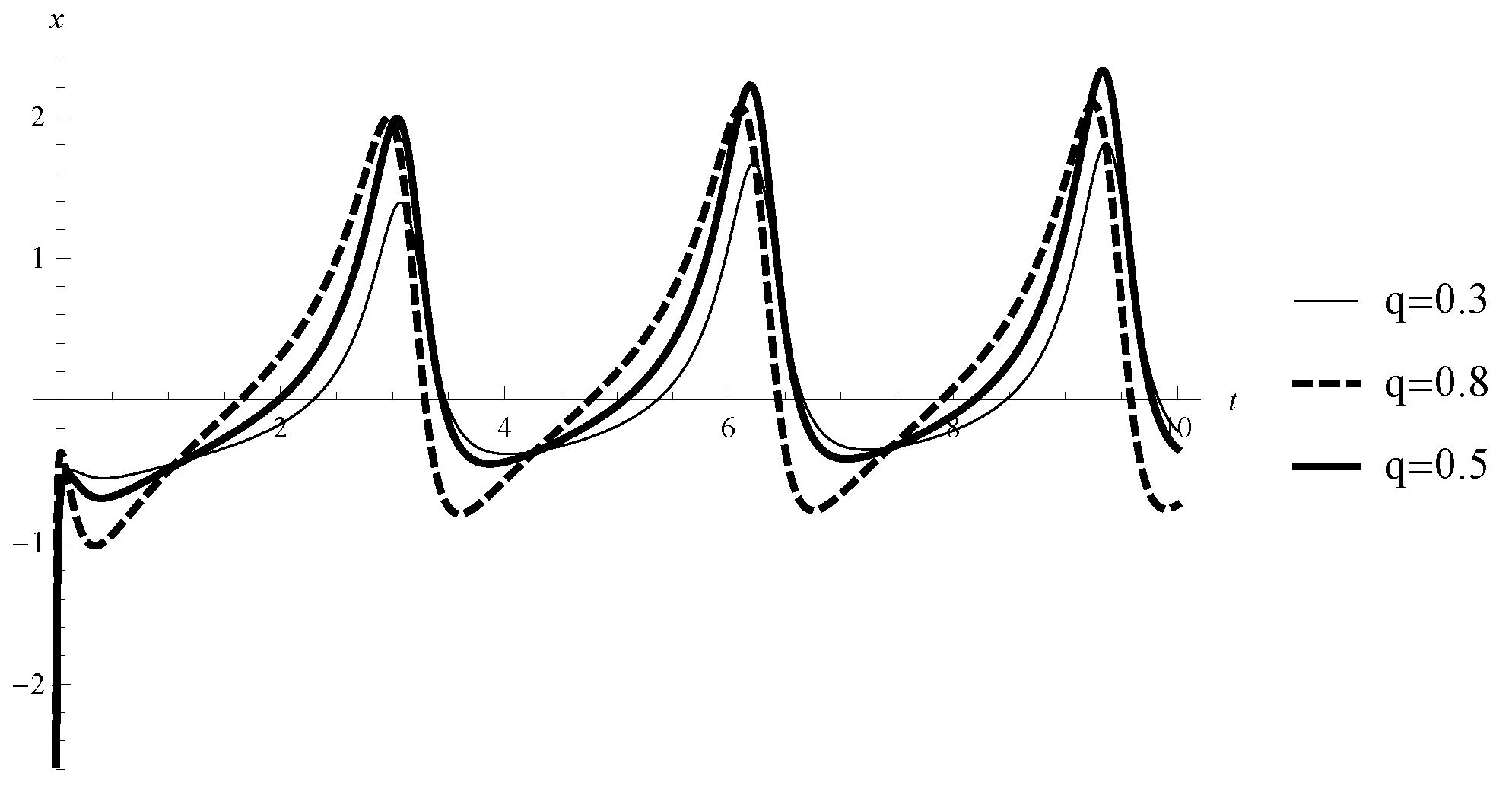
Example 9.
Let n = 1 and consider the scalar FODNN (17) with c ( t ) = 0.55 t q Γ ( 1 q ) ( E q ( t q ) + 0.1 ) + 0.005 E q ( t q ) + 0.1 , I ( t ) 0 , a , b C ( R + , R + ) : a ( t ) + b ( t ) = 0.45 E q ( t q ) E q ( t q ) + 0.1 , the activation functions are the Continuous Tan-Sigmoid Function f ( u ) = g ( u ) = tanh ( u ) = e u e u e u + e u , τ ( t ) r > 0 and the equilibrium point x * = 0 .
Theorem 1 is not applicable since the coefficient before x is not a constant.
Let x ( t ) be a solution of FODNN (17). Then using the inequality | f ( x ) | | x | , x R we get x ( t ) a ( t ) ( f ( x ( t ) ) f ( 0 ) ) a ( t ) x 2 ( t ) . In addition, let t > 0 be such that ( x ( t ) ) 2 = sup s [ r , 0 ] ( x ( s ) ) 2 then | f ( x ( t r ) ) | | x ( t r ) | | x ( t ) | and x ( t ) b ( t ) ( f ( x ( t r ) ) f ( 0 ) ) b ( t ) | x ( t ) ( f ( x ( t r ) ) | b ( t ) ( x ( t ) ) 2 i.e., Assumption 5 is satisfied with ξ ( t ) a ( t ) + b ( t ) . However the inequality ξ ( t ) = a ( t ) + b ( t ) = 0.45 E q ( t q ) E q ( t q ) + 0.1 η ( t ) = c ( t ) = 0.55 t q Γ ( 1 q ) ( E q ( t q ) + 0.1 ) + 0.005 E q ( t q ) + 0.1 is not satisfied (see Figure 4 for q = 0.8 ). Therefore, Theorem 2 cannot be applied.
Consider the function p ( t ) = ( E q ( t q ) + 0.1 ) . Then we get the inequality
p ( t ) η ( t ) + p ( t ) ξ ( t ) + 0.5 0 R L D t q p ( t ) = ( E q ( t q ) + 0.1 ) 0 . 55 t q Γ ( 1 q ) ( E q ( t q ) + 0 . 1 ) + 0 . 005 E q ( t q ) + 0 . 1 + ( E q ( t q ) + 0.1 ) 0.45 E q ( t q ) E q ( t q ) + 0.1 + 0.5 0 R L D t q E q ( t q ) + 0.1 = 0.55 t q Γ ( 1 q ) 0.005 + 0.45 E q ( t q ) + 0.5 E q ( t q ) + 1 . 1 t q Γ ( 1 q ) = 0.55 t q Γ ( 1 q ) 0.005 + 0.45 E q ( t q ) 0.5 E q ( t q ) + 0.55 t q Γ ( 1 q ) = 0.005 0.05 E q ( t q ) = 0.05 E q ( t q ) + 0.1 0.005 .
According to Theorem 3 the equilibrium point x * = 0 of Caputo FODNN (17) is uniformly stable.
Therefore, in the case that the activation functions are not Lipschitz and the coefficients c i are not constants in FODNN, we can use Lyapunov function depending directly on the time variable; its Caputo fractional Dini derivative is applicable to study the stability.

5. Conclusions

Several sufficient conditions are given for stability of the equilibrium point of Caputo fractional order neural networks with delays of order 0 < q < 1 . We study the general case when
-
the transmission delays are time variables;
-
the self-regulating parameters of all units are variable in time;
-
the functions of the connection between two neurons in the network are variable in time bounded functions;
-
the activation function is nonLipschitz (usually in the literature only the case of Lipschitz activation functions is studied).
The investigation is based on applying the fractional Lyapunov approach and various types of Lyapunov functions are discussed (not only the quadratic one as is usually considered in the literature). The presence of the fractional derivative in the model requires an appropriate defined and used derivative of Lyapunov functions among the fractional model. A brief overview of the existing literature and the main types of derivatives among Caputo fractional equations are presented. These types of derivatives are used as an apparatus to study stability properties of the considered Caputo fractional order neural networks for different types of activation functions. Many examples with different types of activation functions such as tanh function, Logit function, continuous Tan-Sigmoid function, are provided to illustrate the practical application of the obtained sufficient conditions.

Author Contributions

The authors have made the same contribution. All authors read and approved the final manuscript.

Acknowledgments

Research was partially supported by Fund MU17-FMI-007, University of Plovdiv “Paisii Hilendarski”.

Conflicts of Interest

The authors declare no conflict of interest.

References

  1. Marcus, C.; Westervelt, R. Stability of analog neural networks with delay. Phys. Rev. A 1989, 39, 347–359. [Google Scholar] [CrossRef]
  2. Chen, D.; Zhang, R.; Liu, X.; Ma, X. Fractional order Lyapunov stability theorem and its applications in synchronization of complex dynamical networks. Commun. Nonlinear Sci. Numer. Simulat. 2014, 19, 4105–4121. [Google Scholar] [CrossRef]
  3. Kaslik, E.; Sivasundaram, S. Nonlinear Dynamics and Chaos in Fractional Order Neural Networks. Neural Netw. 2012, 32, 245–256. [Google Scholar] [CrossRef] [PubMed]
  4. Newman, M.E.J. Communities, modules and large-scale structure in networks. Nat. Phys. 2012, 8, 25–31. [Google Scholar] [CrossRef]
  5. Stigler, J.; Ziegler, F.; Gieseke, A.; Gebhardt, J.C.M.; Rief, M. The complex folding network of single calmodulin molecules. Science 2011, 334, 512–516. [Google Scholar] [CrossRef] [PubMed]
  6. Wanduku, D.; Ladde, G.S. Global properties of a two-scale network stochastic delayed human epidemic dynamic model. Nonlinear Anal.-Real World Appl. 2012, 13, 794–816. [Google Scholar] [CrossRef]
  7. Huang, Y.; Zhang, H.; Wang, Z. Dynamical stability analysis of multiple equilibrium points in time-varying delayed recurrent neural networks with discontinuous activation functions. Neurocomputing 2012, 91, 21–28. [Google Scholar] [CrossRef]
  8. Li, C.; Feng, G. Delay-interval-dependent stability of recurrent neural networks with time-varying delay. Neurocomputing 2009, 72, 1179–1183. [Google Scholar] [CrossRef]
  9. Wu, H.; Wang, L.; Wang, Y.; Niu, P.; Fang, B. Global Mittag-Leffler projective synchronization for fractional-order neural networks: An LMI-based approach. Adv. Differ. Eq. 2016, 2016, 132. [Google Scholar] [CrossRef]
  10. Li, Y.; Chen, Y.; Podlubny, I. Stability of fractional-order nonlinear dynamic systems: Lyapunov direct method and generalized Mittag-Leffler stability. Comput. Math. Appl. 2010, 59, 1810–1821. [Google Scholar] [CrossRef]
  11. Li, Y.; Chen, Y.; Podlubny, I. Mittag-Leffler stability of fractional order nonlinear dynamic systems. Automatica 2009, 45, 1965–1969. [Google Scholar] [CrossRef]
  12. Li, G.; Liu, H. Stability Analysis and Synchronization for a Class of Fractional-Order Neural Networks. Entropy 2006, 18. [Google Scholar] [CrossRef]
  13. Liu, H.; Li, S.; Wang, H.; Huo, Y.; Luo, J. Adaptive Synchronization for a Class of Uncertain Fractional-Order Neural Networks. Entropy 2015, 17, 7185–7200. [Google Scholar] [CrossRef]
  14. Zhang, W.; Wu, R.; Cao, J.; Alsaedi, A.; Hayat, T. Synchronization of a class of fractional-order neural networks with multiple time delays by comparison principles. Nonlinear Anal. Modell. Control 2017, 22, 636–645. [Google Scholar] [CrossRef]
  15. Chen, L.; Chai, Y.; Wu, R.; Ma, T.; Zhai, H. Dynamic analysis of a class of fractional-order neural networks with delay. Neurocomputing 2013, 111, 190–194. [Google Scholar] [CrossRef]
  16. Chen, B.; Chen, J. Razumikhin-type stability theorems for functional fractional-order differential systems and applications. Appl. Math. Comput. 2015, 254, 63–69. [Google Scholar] [CrossRef]
  17. Wang, H.; Yu, Y.; Wen, G. Stability analysis of fractional-order Hopfield neural networks with time delays. Neural Netw. 2014, 55, 98–109. [Google Scholar] [CrossRef] [PubMed]
  18. Zhang, W.; Cao, J.; Chen, D.; Alsaadi, F.E. Synchronization in fractional-order complex-valued delayed neural networks. Entropy 2018, 20. [Google Scholar] [CrossRef]
  19. Bao, H.; Park, J.H.; Cao, J. Synchronization of fractional-order complex-valued neural networks with time delay. Neural Netw. 2016, 81, 16–28. [Google Scholar] [CrossRef] [PubMed]
  20. Wu, R.-C.; Hei, X.-D.; Chen, L.-P. Finite-time stability of fractional-order neural networks with delay. Commun. Theor. Phys. 2013, 60, 189–193. [Google Scholar] [CrossRef]
  21. Yang, X.; Song, Q.; Liu, Y.; Zhao, Z. Finite-time stability analysis of fractional-order neural networks with delay. Neurocomputing 2015, 152, 19–26. [Google Scholar] [CrossRef]
  22. Alofi, A.; Cao, J.; Elaiw, A.; Al-Mazrooei, A. Delay-Dependent Stability Criterion of Caputo Fractional Neural Networks with Distributed Delay. Discr. Dynam. Nat. Soc. 2014, 2014, 529358. [Google Scholar] [CrossRef]
  23. Podlubny, I. Fractional Differential Equations; Academic Press: San Diego, CA, USA, 1999. [Google Scholar]
  24. Stamova, I.; Stamov, G. Functional and Impulsive Differential Equations of Fractional Order: Qualitative Analysis and Applications; CRC Press: Boca Raton, FL, USA, 2016. [Google Scholar]
  25. Devi, J.V.; Rae, F.A.M.; Drici, Z. Variational Lyapunov method for fractional differential equations. Comput. Math. Appl. 2012, 64, 2982–2989. [Google Scholar] [CrossRef]
  26. Agarwal, R.; Hristova, S.; O’Regan, D. A survey of Lyapunov functions, stability and impulsive Caputo fractional differential equations. Fract. Calc. Appl. Anal. 2016, 19, 290–318. [Google Scholar] [CrossRef]
  27. Agarwal, R.; Hristova, S.; O’Regan, D. Lyapunov functions and strict stability of Caputo fractional differential equations. Adv. Differ. Eq. 2015, 2015, 346. [Google Scholar] [CrossRef]
  28. Agarwal, R.; O’Regan, D.; Hristova, S.; Cicek, M. Practical stability with respect to initial time difference for Caputo fractional differential equations. Commun. Nonlinear Sci. Numer. Simulat. 2017, 42, 106–120. [Google Scholar] [CrossRef]
  29. Duarte-Mermoud, M.A.; Aguila-Camacho, N.; Gallegos, J.A.; Castro-Linares, R. Using general quadratic Lyapunov functions to prove Lyapunov uniform stability for fractional order systems. Commun. Nonlinear Sci. Numer. Simulat. 2015, 22, 650–659. [Google Scholar] [CrossRef]
  30. Stamova, I. On the Lyapunov theory for functional differential equations of fractional order. Proc. Am. Math. Soc. 2016, 144, 1581–1593. [Google Scholar] [CrossRef]
  31. Stamova, I.; Simeonov, S. Delayed Reaction-Diffusion Cellular Neural Networks of Fractional Order: Mittag-Leffler Stability and Synchronization. J. Comput. Nonlinear Dyn. 2017, 13, 011015. [Google Scholar] [CrossRef]
  32. Gelfand, I.M. General theory of hypergeometric functions. Doklady Akademii Nauk SSSR 1986, 288, 14–18, (English translation in collected papers, volume III). [Google Scholar]
  33. Rahimi, A.; Recht, B. Weighted sums of random kitchen sinks: Replacing minimization with randomization in learning. Adv. Neural Inf. Process. Syst. 2008, 21, 1313–1320. [Google Scholar]
  34. Agarwal, R.; Hristova, S.; O’Regan, D. Lyapunov functions and stability of Caputo fractional differential equations with delays. Unpublished work. 2018. [Google Scholar]
  35. Li, R.; Cao, J.; Alsaedi, A.; Alsaadi, F. Stability analysis of fractional-order delayed neural networks. Nonlinear Anal. Model. Control 2017, 22, 505–520. [Google Scholar] [CrossRef]
Figure 1. Example 2. Graph of the function g ( t ) + 0.1 for various values of q.
Axioms 07 00030 g001
Figure 2. Example 5. Graph of the function f ( t ) = 2 erf 1 ( 2 t 1 ) .
Axioms 07 00030 g002
Figure 3. Example 5. Graph of the function f ( u ) = log u 1 u .
Axioms 07 00030 g003
Figure 4. Example 9. Graph of the functions ξ ( t ) and η ( t ) for q = 0.8 .
Axioms 07 00030 g004

