1. Introduction
The purpose of our paper is to identify a unifying framework in infinite-dimensional analysis which involves a core duality notion. There are two elements to our point of view: (i) presentation of the general setting of duality and representation theory, and (ii) detailed applications for two areas, often considered disparate. The first is stochastic analysis, and the second is from the theory of von Neumann algebras (Tomita-Takesaki theory), see, e.g., [
1,
2]. We feel that this viewpoint is useful as it adds unity to the study of infinite-dimensional analysis; and further, because researchers in one of these two areas usually do not explore the other, or are even unfamiliar with the connections.
We study densely defined unbounded operators acting between different Hilbert spaces, and for these, we introduce a notion of symmetric (closable) pairs of operators. The purpose of our paper is to give applications to themes at the cross road of commutation relations (operator theory) and stochastic calculus. While both subjects have been studied extensively, our aim is to show that the notion of closable pairs from the theory of unbounded operators serves to unify the two areas. Both areas are important in mathematical physics, but researchers familiar with operator theory typically do not appreciate the implications of results on unbounded operators and their commutators for stochastic analysis; and vice versa.
Both the study of quantum fields, and of quantum statistical mechanics, entails families of representations of the canonical commutation relations (CCRs). In the case of an infinite number of degrees of freedom, it is known that we have existence of many inequivalent representations of the CCRs. Among the representations, some describe such things as a nonrelativistic infinite free Bose gas of uniform density. However, the representations of the CCRs play an equally important role in the kind of infinite-dimensional analysis currently used in a calculus of variation approach to Gaussian fields, Itō integrals, including the Malliavin calculus. In the literature, the infinite-dimensional stochastic operators of derivatives and stochastic integrals are usually taken as the starting point, and the representations of the CCRs are an afterthought. Here we turn the tables. As a consequence of this, we are able to obtain a number of explicit results in an associated multi-variable spectral theory. Some of the issues involved are subtle because the operators in the representations under consideration are unbounded (by necessity), and, as a result, one must deal with delicate issues of domains of families of operators and their extensions.
The representations we study result from the Gelfand-Naimark-Segal construction (GNS) applied to certain states on the CCR-algebra. Our conclusions and main results regarding this family of CCR representations (details below, especially
Section 4 and
Section 5) hold in the general setting of Gaussian fields. However, for the benefit of readers, we have also included an illustration dealing with the simplest case, that of the standard Brownian/Wiener process. Many arguments in the special case carry over to general Gaussian fields
mutatis mutandis. In the Brownian case, our initial Hilbert space will be
.
From the initial Hilbert space
, we build the *-algebra
as in
Section 2.2. We will show that the Fock state on
corresponds to the Wiener measure
. Moreover the corresponding representation
π of
will be acting on the Hilbert space
in such a way that for every
k in
, the operator
is the Malliavin derivative in the direction of
k. We caution that the representations of the *-algebra
are by unbounded operators, but the operators in the range of the representations will be defined on a single common dense domain.
Example: There are two ways to think of systems of generators for the CCR-algebra over a fixed infinite-dimensional Hilbert space (“CCR” is short for canonical commutation relations):
- (i)
an infinite-dimensional Lie algebra, or
- (ii)
an associative *-algebra.
With this in mind, (ii) will simply be the universal enveloping algebra of (i); see [
3]. While there is also an infinite-dimensional “Lie” group corresponding to (i), so far, we have not found it as useful as the Lie algebra itself.
All this, and related ideas, supply us with tools for an infinite-dimensional stochastic calculus. It fits in with what is called Malliavin calculus, but our present approach is different, and more natural from our point of view; and as corollaries, we obtain new and explicit results in multi-variable spectral theory which we feel are of independent interest.
There is one particular representation of the CCR version of (i) and (ii) which is especially useful for stochastic calculus. In the present paper, we call this representation the Fock vacuum-state representation. One way of realizing the representations is abstract: Begin with the Fock vacuum state (or any other state), and then pass to the corresponding GNS representation. The other way is to realize the representation with the use of a choice of a Wiener -space. We prove that these two realizations are unitarily equivalent.
By stochastic calculus we mean stochastic derivatives (e.g., Malliavin derivatives), and integrals (e.g., Itō-integrals). The paper begins with the task of realizing a certain stochastic derivative operator as a closable operator acting between two Hilbert spaces.
There is an extensive literature on quantum stochastic calculus based on the Fock, and other representations, of the CCR including its relation to Malliavin calculus. The list of authors includes R. Hudson, K. R. Parthasarathy and collaborators. We refer the reader to the papers [
4,
5,
6,
7,
8], and also see [
9,
10]. Of more recent papers dealing with results which have motivated our present paper are [
11,
12,
13,
14,
15,
16,
17,
18,
19,
20,
21,
22,
23,
24,
25,
26].
2. Unbounded Operators and the CCR-algebra
2.1. Unbounded Operators between Different Hilbert Spaces: Closable Pairs
While the theory of unbounded operators has been focused on spectral theory where it is then natural to consider the setting of linear endomorphisms with dense domain in a fixed Hilbert space; many applications entail operators between distinct Hilbert spaces, say and . Typically the facts given about the two differ greatly from one Hilbert space to the next.
Let , , be two complex Hilbert spaces. The respective inner products will be written , with the subscript to identify the Hilbert space in question.
Definition 2.1. A linear operator T from to is a pair , T, where is a linear subspace in , and is well-defined for all .
We say that
is the domain of
T, and
is the graph.
If the closure
is the graph of a linear operator, we say that
T is
closable. By closure, we shall refer to closure in the norm of
,
i.e.,
If is dense in , we say that T is densely defined.
Definition 2.2 (The adjoint operator).
Let
be a densely defined operator, consider the subspace
defined as follows:
Then, by Riesz’ theorem, there is a unique
s.t.
we set
.
is called the
adjoint of
T.
Lemma 2.3. Given a densely defined operator , then T is closable if and only if is dense in .
Remark 2.4 (Notation and Facts).
- 1.
The abbreviated notation ![Axioms 05 00012 i001]() will be used when the domains of T and are understood from the context.
will be used when the domains of T and are understood from the context. - 2.
Let T be an operator and , , two given Hilbert spaces. Assume is dense in , and that T is closable.
Then there is a unique closed
operator, denoted such thatwhere “—” on the RHS in Equation (5) refers to norm closure in , see Equation (2). - 3.
It may happen that . See Example 2.6 below.
Definition 2.5 (closable pairs).
Let
and
be two Hilbert spaces with respective inner products
,
; let
,
, be two dense linear subspaces; and let
be linear operators such that
Then both operators
and
are closable. The closures
, and
satisfy
We say the system
is a
closable pair. (Also see Definition 3.5.)
Example 2.6. An operator with dense domain s.t. , i.e., “extremely” non-closable.
Set , , where and are two mutually singular measures on a fixed locally compact measurable space, say X. The space is dense in both and in with respect to the two -norms. Then, the identity mapping , , becomes a Hilbert space operator .
Using Definition 2.2, we see that
is in
iff
such that
Since
is dense in both
-spaces, we get
where
.
Now suppose in , then there is a subset s.t. on A, , and . But , and since . This contradiction proves that ; and in particular T is unbounded and non-closable.
Theorem 2.7. Let be a densely defined operator, and assume that is dense in , i.e., T is closable, then both of the operators and are densely defined, and both are selfadjoint.
Moreover, there is a partial isometry with initial space in and final space in such that(Equation (10) is called the polar decomposition of T.) 2.2. The CCR-algebra, and the Fock Representations
There are two *-algebras built functorially from a fixed (single) Hilbert space
; often called the one-particle Hilbert space (in physics). The dimension
is called
the number of degrees of freedom. The case of interest here is when
(countably infinite). The two *-algebras are called the CAR, and the CCR-algebras, and they are extensively studied; see, e.g., [
2]. Of the two, only CAR(
) is a
-algebra. The operators arising from representations of CCR(
) will be
unbounded, but still having a common dense domain in the respective representation Hilbert spaces. In both cases, we have a Fock representation. For CCR(
), it is realized in the symmetric Fock space
. There are many other representations, inequivalent to the respective Fock representations.
Let
be as above. The CCR(
) is generated axiomatically by a system,
,
,
, subject to
Notation. In Equation (
11),
denotes the commutator. More specifically, if
are elements in a *-algebra, set
.
The
Fock States on the CCR-algebra are specified as follows:
with the vacuum property
For the corresponding Fock representations
π we have:
where
on the RHS of Equation (
14) refers to the identity operator.
Some relevant papers regarding the CCR-algebra and its representations are [
28,
29,
30,
31,
32,
33,
34,
35].
2.3. An Infinite-dimensional Lie Algebra
Let be a separable Hilbert space, i.e., , and let be the corresponding CCR-algebra. As above, its generators are denoted and , for . We shall need the following:
Proposition 2.8. - 1.
The “quadratic” elements in of the form , , span a Lie algebra under the commutator bracket.
- 2.
We havefor all . - 3.
If is an ONB in , then the non-zero commutators are as follows: Set , then, for , we haveAll other commutators vanish; in particular, spans an abelian sub-Lie algebra in . Note further that, when , then the three elementsspan (over ) an isomorphic copy of the Lie algebra . - 4.
The Lie algebra generated by the first-order elements and for , is called the Heisenberg Lie algebra . It is normalized by ; indeed we have:
Proof. The verification of each of the four assertions (
1)–(
4) uses only the fixed axioms for the CCR,
i.e.,
where
denotes the unit-element in
. ☐
Corollary 2.9. Let be the CCR-algebra, generators , , , and let denote the commutator Lie bracket; then, for all , and all (= the n-variable polynomials over ), we have Proof. The verification of Equation (
20) uses only the axioms for the CCR,
i.e., the commutation relations (
19) above, plus a little combinatorics. ☐
We shall now return to a stochastic variation of formula (
20), the so called Malliavin derivative in the direction
k. In this, the system
in Equation (
20) instead takes the form of a multivariate Gaussian random variable.
2.4. Gaussian Hilbert Space
The literature on Gaussian Hilbert space, white noise analysis, and its relevance to Malliavin calculus is vast; we limit ourselves here to citing [
17,
36,
37,
38,
39,
40,
41], and the papers cited there.
Setting and Notation:
: a fixed real Hilbert space
: a fixed probability space
: the Hilbert space , also denoted by
: the mean or expectation functional, where
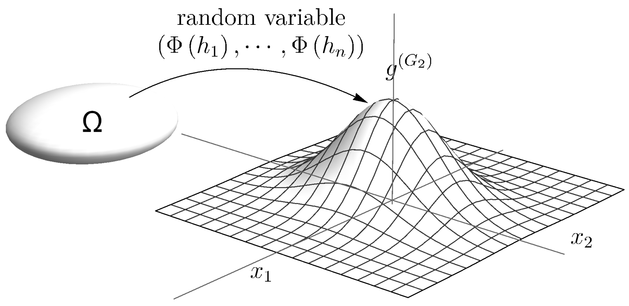
Definition 2.10. Fix a real Hilbert space and a given probability space . We say the pair is a Gaussian Hilbert space.
A
Gaussian field is a linear mapping
, such that
is a Gaussian process indexed by
satisfying:
, ;
,
, the random variable
is jointly Gaussian, with
i.e.,
= the covariance matrix. (For the existence of Gaussian fields, see the discussion below.)
Remark 2.11. For all finite systems , set , called the Gramian. Assume non-singular for convenience, so that . Then there is an associated Gaussian density on ,The condition in Equation (21) assumes that for all continuous functions (e.g., polynomials), we havewhere , and = Lebesgue measure on . See Figure 1 for an illustration. In particular, for , , and , we then get , i.e., the inner product in .
For our applications, we need the following facts about Gaussian fields.
Fix a Hilbert space
over
with inner product
. Then (see [
17,
42,
43]) there is a
probability space , depending on
, and a
real linear mapping
,
i.e., a Gaussian field as specified in Definition 2.10, satisfying
It follows from the literature (see also [
44]) that
may be thought of as a generalized Itō-integral. One approach to this is to select a nuclear Fréchet space
with dual
such that
forms a Gelfand triple. In this case we may take
, and
,
, to be the extension of the mapping
defined initially only for
, but, with the use of (
26), now extended, via (
24), from
to
. See also Example 2.13 below.
Example 2.12. Fix a measure space
. Let
be a Gaussian field such tha
where
,
; and
denotes the characteristic function. In this case,
.
Then we have
,
i.e., the Itō-integral, and the following holds:
for all
. Eq. (
27) is known as the Itō-isometry.
Example 2.13 (The special case of Brownian motion).
There are many ways of realizing a Gaussian probability space . Two candidates for the sample space:
- Case 1.
Standard Brownian motion process: , = σ-algebra generated by cylinder sets, = Wiener measure. Set , ; and , .
- Case 2.
The Gelfand triples:
, where
Set
,
=
σ-algebra generated by cylinder sets of
, and define
Note Φ is defined by extending the duality
to
. The probability measure
is defined from
by Minlos’ theorem [
17,
42].
Definition 2.14. Let
be the dense subspace spanned by functions
F, where
iff
,
, and
= the polynomial ring, such that
(See the diagram below.) The case of
corresponds to the constant function
on Ω. Note that
.
Lemma 2.15. The polynomial fields in Definition 2.14 form a dense subspace in .
Proof. The easiest argument below takes advantage of the isometric isomorphism of
with the symmetric Fock space
For
,
, there is a unique vector
such that
Moreover,
extends by linearity and closure to a unitary isomorphism
, mapping onto
(also see Equation (
73) in Theorem 3.30.) Hence
is dense in
, as
is dense in
. ☐
Lemma 2.16. Let be a real Hilbert space, and let be an associated Gaussian field. For , let be a system of linearly independent vectors in . Then, for polynomials , the following two conditions are equivalent: Proof. Let
be the Gramian matrix. We have
. Let
be the corresponding Gaussian density; see Equation (
22), and
Figure 1. Then the following are equivalent:
in ;
;
a.e. x w.r.t. the Lebesgue measure in ;
,
;
i.e., Equation (
29) holds.
☐
3. The Malliavin Derivatives
Below we give an application of the closability criterion for linear operators
T between different Hilbert spaces
and
, but having dense domain in the first Hilbert space. In this application, we shall take for
T to be the so called Malliavin derivative. The setting for it is that of the Wiener process. For the Hilbert space
we shall take the
-space,
where
is generalized Wiener measure. Below we shall outline the basics of the Malliavin derivative, and we shall specify the two Hilbert spaces corresponding to the setting of Theorem 2.7. We also stress that the literature on Malliavin calculus and its applications is vast, see, e.g., [
17,
36,
45,
46,
47].
Settings. It will be convenient for us to work with the real Hilbert spaces.
Let be as specified in Definition 2.10, i.e., we consider the Gaussian field Φ. Fix a real Hilbert space with . Set , and , i.e., vector valued random variables.
For
, the inner product
is
where
is the mean or expectation functional.
On
, we have the tensor product inner product: If
,
,
, then
Equivalently, if
,
, are measurable functions on Ω, we set
where it is assumed that
Remark 3.1. In the special case of standard Brownian motion, we have , and set (= the Itō-integral), for all . Recall we then haveor equivalently (the Itō-isometry),The consideration above also works in the context of general Gaussian fields; see Section 2.4. Definition 3.2. Let be the dense subspace in as in Definition 2.14. The operator (= Malliavin derivative) with is specified as follows:
For
,
i.e.,
,
a polynomial in
n real variables, and
, where
Set
In the following two remarks we outline the argument for why the expression for
in Equation (
37) is independent of the chosen representation (
36) for the particular
F. Recall that
F is in the domain
of
T. Without some careful justification, it is not even clear that
T, as given, defines a linear operator on its dense domain
. The key steps in the argument to follow will be the result (
41) in Theorem 3.8 below, and the discussion to follow.
There is an alternative argument, based instead on Corollary 2.9; see also
Section 5 below.
Remark 3.3. It is non-trivial that the formula in Equation (37) defines a linear operator. Reason: On the LHS in Equation (37), the representation of F from (36) is not unique. So we must show that ⟹ as well. (The dual pair analysis below (see Definition 3.6) is good for this purpose.) Suppose has two representations corresponding to systems of vectors , and , with polynomials , and , whereWe must then verify the identity: The significance of the next result is the implication (38) ⟹ (39), valid for all choices of representations of the same . The conclusion from (41) in Theorem 3.8 is that the following holds for all :Moreover, with a refinement of the argument, we arrive at the identityvalid for all , and all . However, is dense in w.r.t. the tensor-Hilbert norm in (see (31)); and we get the desired identity (39) for any two representations of F. Remark 3.4. An easy case where (38) ⟹ (39) can be verified “by hand”: Let with fixed. We can then pick the two systems and with , and . A direct calculus argument shows that .
We now resume the argument for the general case.
Definition 3.5 (symmetric pair).
For , let be two Hilbert spaces, and suppose are given dense subspaces.
We say that a pair of operators
forms a
symmetric pair if
, and
; and moreover,
holds for
,
. (Also see Definition 2.5.)
It is immediate that (
40) may be rewritten in the form of containment of graphs:
In that case, both
S and
T are
closable. We say that a symmetric pair is
maximal if
and
.
We will establish the following two assertions:
Indeed T from Definition 3.2 is a well-defined linear operator from to .
Moreover, is a maximal symmetric pair (see Definitions 3.5 and 3.6).
Definition 3.6. Let
be the Malliavin derivative with
, see Definition 3.2. Set
= algebraic tensor product, and on
, set
where
= the operator of multiplication by
.
Note that both operators S and T are linear and well defined on their respective dense domains, , . For density, see Lemma 2.15.
It is a “modern version” of ideas in the literature on analysis of Gaussian processes; but we are adding to it, giving it a twist in the direction of multi-variable operator theory, representation theory, and especially to representations of infinite-dimensional algebras on generators and relations. Moreover our results apply to more general Gaussian processes than covered so far.
Lemma 3.7. Let be the pair of operators specified above in Definition 3.6. Then it is a symmetric pair, i.e.,Equivalently, In particular, we have , and (containment of graphs.) Moreover, the two operators and are selfadjoint. (For the last conclusion in the lemma, see Theorem 2.7.)
Theorem 3.8. Let be the Malliavin derivative, i.e., T is an unbounded closable operator with dense domain consisting of the span of all the functions F from (36). Then, for all , and , we have Proof. We shall prove (
41) in several steps. Once (
41) is established, then there is a recursive argument which yields a dense subspace in
, contained in
; and so
T is closable.
Moreover, formula (
41) yields directly the evaluation of
as follows: If
, set
where
denotes the constant function “one” on Ω. We get
The same argument works for any Gaussian field; see Definition 2.10. We refer to the literature [
17,
36] for details.
The proof of (
41) works for any Gaussian process
indexed by an arbitrary Hilbert space
with the inner product
as the covariance kernel.
Formula (
41) will be established as follows: Let
F and
be as in Equation (
36) and Equation (
37).
Step 1. For every , the polynomial ring is invariant under matrix substitution , where M is an matrix over .
Step 2. Hence, in considering (
41) for
,
, we may diagonalize the
Gram matrix
; thus without loss of generality, we may assume that the system
is orthogonal and normalized,
i.e., that
and we may take
in
.
Step 3. With this simplification, we now compute the LHS in (
41). We note that the joint distribution of
is thus the standard Gaussian kernel in
,
i.e.,
with
. We have
by calculus.
Step 4. A direct computation yields
which is the desired conclusion (
41). ☐
Corollary 3.9. Let , , and be as in Theorem 3.8, i.e., T is the Malliavin derivative. Then, for all , we have for the closure of T the following:Here denotes the graph-closure of T. Proof. Equation (
46) and Equation (
47) follow immediately from (
41) and a polynomial approximation to
see (
36). In particular,
, and
is well defined.
For Equation (
48), we use the facts for the Gaussians:
☐
Example 3.10. Let
,
. We have
and similarly,
Let be the symmetric pair, we then have the inclusion , i.e., containment of the operator graphs, . In fact, we have
Corollary 3.11. .
Proof. We will show that , where ⊖ stands for the orthogonal complement in the direct sum-inner product of . Recall that , and .
Using (
46), we will prove that if
, and
which is equivalent to
But it is know that for the Gaussian filed,
is dense in
, and so (
49) implies that
, which is the desired conclusion.
We can finish the proof of the corollary with an application of Girsanov’s theorem, see e.g., [
36] and [
48]. By this result, we have a measurable action
τ of
on
,
i.e.,
(see also sect 5 below) s.t.
for all
, and
with
Returning to (
49). An application of (
51) to (
49) yields:
where we have used “
” for the action in (
50). Since
τ in (
50) is an action by measure-automorphisms, (
52) implies
again with
arbitrary. If
in
, then the second term in (
53) would be independent of
k which is impossible with
. But if
, then
(in
) by (
53); and so the proof is completed. ☐
Remark 3.12. We recall the definition of the domain of the closure . The following is a necessary and sufficient condition for an to be in the domain of :
⟺ ∃
a sequence s.t.When (54) holds, we have:where the limit on the RHS in (55) is in the Hilbert norm of .Corollary 3.13. Let be as above, and let T and S be the two operators from Corollary 3.11. Then, for the domain of , we have the following:
For random variables F in , the following two conditions are equivalent:;
s.t.holds for . Recallequivalently,for all , and all .
Proof. Immediate from the previous corollary. ☐
3.1. A Derivation on the Algebra
The study of unbounded derivations has many applications in mathematical physics; in particular in making precise the time dependence of quantum observables,
i.e., the dynamics in the Schrödinger picture; —in more detail, in the problem of constructing dynamics in statistical mechanics. An early application of unbounded derivations (in the commutative case) can be found in the work of Silov [
49]; and the later study of unbounded derivations in non-commutative
-algebras is outlined in [
2]. There is a rich variety in unbounded derivations, because of the role they play in applications to dynamical systems in quantum physics.
However, previously the theory of unbounded derivations has not yet been applied systematically to stochastic analysis in the sense of Malliavin. In the present section, we turn to this. We begin with the following:
Lemma 3.14 (Leibniz-Malliavin).
Let be the Malliavin derivative from Equation (36) and Equation (37). Then,- 1.
, given by (36), is an algebra
of functions on Ω under pointwise product, i.e., , . - 2.
is a module over where (= vector valued -random variables.)
- 3.
Moreover,i.e., T is a module-derivation.
Notation. The Equation (
56) is called the Leibniz-rule. By the Leibniz, we refer to the traditional rule of Leibniz for the derivative of a product. And the Malliavin derivative is thus an infinite-dimensional extension of Leibniz calculus.
Proof. To show that is an algebra under pointwise multiplication, the following trick is useful. It follows from finite-dimensional Hilbert space geometry.
Let
be as in Definition 2.14. Then
,
, such that
That is, the same system
may be chosen for the two functions
F and
G.
For the pointwise product, we have
i.e., the product in
with substitution of the random variable
Equation (
56) ⟺
, which is the usual Leibniz rule applied to polynomials. Note that
☐
Remark 3.15. There is an extensive literature on the theory of densely defined unbounded derivations in -algebras. This includes both the cases of abelian and non-abelian *-algebras. Moreover, this study includes both derivations in these algebras, as well as the parallel study of module derivations. Therefore, the case of the Malliavin derivative is in fact a special case of this study. Readers interested in details are referred to [1,2,50,51]. Definition 3.16. Let
be a Gaussian field, and
T be the Malliavin derivative with
. For all
, set
In particular, let
be as in (
36), then
Corollary 3.17. is a derivative on , i.e., Proof. Follows from Equation (
56). ☐
Corollary 3.18. Let be a Gaussian field. Fix , and let be the Malliavin derivative in the k direction. Then on we have Proof. For all
, we have
which yields the assertion in (
59). Equation (
60) now follows from (
59) and the fact that
. ☐
Definition 3.19. Let
be a Gaussian field. For all
, let
be Malliavin derivative in the
k-direction (
57). Assume
is separable,
i.e.,
. For every ONB
in
, let
N is the CCR number operator. See
Section 4 below.
Example 3.20. , since
,
. Similarly,
To see this, note that
which is (
62). The verification of (
63) is similar.
Theorem 3.21. Let be an ONB in , then Proof. Note the span of
is dense in
, and both sides of (
64) agree on
,
. Indeed, by (
61),
☐
Corollary 3.22. Let . Specialize to the case of , and consider , , ; then Proof. A direct application of the formulas of and ☐
Remark 3.23. If in (65), then the RHS in (65) is obtained by a substitution of the real valued random variable into the deterministic functionThen Equation (65) may be rewritten as Corollary 3.24. If , , denotes the Hermite polynomials on , then we get for , , the following eigenvalues Proof. It is well-known that the Hermite polynomials
satisfies
and so (
68) follows from a substitution of (
69) into (
67). ☐
Theorem 3.25.
The spectrum of , as an operator in , is as follows: Proof. We saw that the -representation is unitarily equivalent to the Fock vacuum representation, and . ☐
3.2. Infinite-dimensional Δ and
Corollary 3.26. Let be a Gaussian field, and let T be the Malliavin derivative, . Then, for all (see Definition 3.2), we havewhich is abbreviated
For the general theory of infinite-dimensional Laplacians, see, e.g., [
52].
Proof. (Sketch) We may assume the system
is orthonormal,
i.e.,
. Hence, for
, we have
which is the assertion. For details, see the proof of Theorem 3.8. ☐
Definition 3.27. Let
be a Gaussian field. On the dense domain
, we define the Φ-gradient by
for all
. (Note that
is an unbounded operator in
, and
.)
Lemma 3.28. Let be the Φ
-gradient from Definition 3.27. The adjoint operator , i.e., the Φ
-divergence, is given as follows: Proof. Fix
as in Definition 3.2. Then
,
, and
, such that
Further assume that
.
In the calculation below, we use the following notation:
,
= Lebesgue measure, and
= standard Gaussian distribution in
, see (
44).
Then, we have
which is the desired conclusion in (
72). ☐
Remark 3.29. Note is not
a derivation. In fact, we havefor all , and all . However, the divergence operator does satisfy the Leibniz rule, i.e., 3.3. Realization of the operators
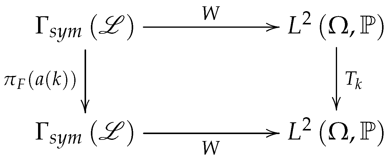
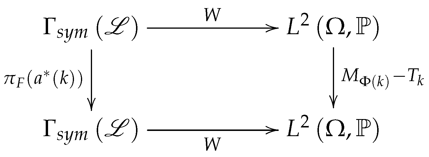
Theorem 3.30. Let be the Fock state on , see Equation (12) and Equation (13), and let denote the corresponding (Fock space) representation, acting on , see Lemma 2.15. Let be the isomorphism given byHere denotes the Gaussian Hilbert space corresponding to ; see Definition 2.10. For vectors , let denote the Malliavin derivative in the direction k; see Definition 3.2. We then have the following realizations:valid for all , where the two identities Equation (74) and Equation (75) hold on the dense domain from Lemma 2.15. In the proof of the theorem, we make use of the following:
Lemma 3.32. Let , , and (= the Fock vacuum state) be as above. Then, for all , and all , , we have the following identity:where the summation on the RHS in (76) is over the symmetric group of all permutations of . (In the case of the CARs, the analogous expression on the RHS will instead be a determinant.) Proof. We leave the proof of the lemma to the reader; it is also contained in [
2]. ☐
Remark 3.33. In physics-lingo, we say that the vacuum-state is determined by its two-point functions
Proof of Theorem 3.30. We shall only give the details for formula (
74). The modifications needed for (
75) will be left to the reader.
Since
W in (
73) is an isomorphic isomorphism,
i.e., a unitary operator from
onto
, we may show instead that
holds on the dense subspace of all finite symmetric tensor polynomials in
; or equivalently on the dense subspace in
spanned by
see also Lemma 2.15. We now compute (
77) on the vectors
in (
78):
valid for all
. ☐
3.4. The Unitary Group
For a given Gaussian field , we studied the -algebra, and the operators associated with its Fock-vacuum representation.
From the determination of Φ by
we deduce that
satisfies the following covariance with respect to the group
of all unitary operators
.
We shall need the following:
Definition 3.34. We say that
iff the following three conditions hold:
is defined a.e. on Ω, and .
; more precisely,
where
, i.e., α is a measure preserving automorphism.
Note that when Equation (
1)–Equation (
3) hold for
α, then we have the unitary operators
in
,
or more precisely,
valid for all
.
Theorem 3.35. - 1.
For every (= the unitary group of
), there is a unique s.t.or equivalently (see (81)) - 2.
If is the Malliavin derivative from Definition 3.2, then we have:
Proof. The first conclusion in the theorem is immediate from the above discussion, and we now turn to the covariance formula (
84).
Note that (
84) involves unbounded operators, and it holds on the dense subspace
in
from Lemma 2.15. Hence it is enough to verify (
84) on vectors in
of the form
,
. Using Lemma 2.15, we then get:
which is the desired conclusion. ☐
4. The Fock-State, and Representation of CCR, Realized as Malliavin Calculus
We now resume our analysis of the representation of the canonical commutation relations (CCR)-algebra induced by the canonical Fock state (see (
11)). In our analysis below, we shall make use of the following details: Brownian motion, Itō-integrals, and the Malliavin derivative.
The general setting. Let
be a fixed Hilbert space, and let
be the *-algebra on the generators
,
,
, and subject to the relations for the CCR-algebra, see
Section 2.2:
where
is the commutator bracket.
A representation
π of
consists of a fixed Hilbert space
(the representation space), a dense subspace
, and a *-homomorphism
such that
The representation axiom entails the commutator properties resulting from Equation (
85) and Equation (
86); in particular
π satisfies
,
; where
.
In the application below, we take
, and
where
is the standard Wiener probability space, and
For
, we set
The dense subspace is generated by the polynomial fields:
For
,
,
a polynomial in
n real variables, set
It follows from Lemma 3.14 that
is an algebra under pointwise product and that
,
. Equivalently,
is a derivation in the algebra
(relative to pointwise product.)
Theorem 4.1. With the operators , , we get a *-representation , i.e., = the Malliavin derivative in the direction k, Proof. The proof begins with the following lemma. ☐
Lemma 4.2. Let π, , and be as above. For , we shall identify with the unbounded multiplication operator in :For , we have ; or in abbreviated form:valid on the dense domain . Proof. This follows from the following computation for , .
Setting
, we have
Hence
, and
, which is the desired conclusion (
96). ☐
Proof of Theorem 4.1 continued. It is clear that the operators
form a commuting family. Hence on
, we have for
,
:
which is the desired commutation relation (
86).
The remaining check on the statements in the theorem are now immediate. ☐
Corollary 4.3. The state on which is induced by π and the constant function in is the Fock-vacuum-state, .
Proof. The assertion will follow once we verify the following two conditions:
and
for all
.
This in turn is a consequence of our discussion of Equation (
12) and Equation (
13) above: The Fock state
is determined by these two conditions. The assertions (
97) and (
98) follow from
, and
. See (
42). ☐
Corollary 4.4. For we get a family of selfadjoint multiplication operators on where . Moreover, the von Neumann algebra generated by these operators is , i.e., the maximal abelian -algebra of all multiplication operators in .
Remark 4.5. In our considerations of representations π of in a Hilbert space , we require the following five axioms satisfied:- 1.
a dense subspace ;
- 2.
, i.e., ;
- 3.
, ;
- 4.
, ; and
- 5.
, .
Note that in our assignment for the operators , and in Lemma 4.2, we have all the conditions (1)–(5) satisfied. We say that π is a selfadjoint representation
. If alternatively, we definewith the following modification:then this ρ will satisfy (1)–(3), andbut then ; i.e., non-containment of the respective graphs. One generally says that the representation π is (formally) selfadjoint, while the second representation ρ is not.


