Complexity L0-Penalized M-Estimation: Consistency in More Dimensions

Abstract

We study the asymptotics in $L^2$ for complexity penalized least squares regression for the discrete approximation of finite-dimensional signals on continuous domains—e.g., images—by piecewise smooth functions. We introduce a fairly general setting, which comprises most of the presently popular partitions of signal or image domains, like interval, wedgelet or related partitions, as well as Delaunay triangulations. Then, we prove consistency and derive convergence rates. Finally, we illustrate by way of relevant examples that the abstract results are useful for many applications.

1. Introduction

We are going to study the consistency of special complexity penalized least squares estimators for noisy observations of finite-dimensional signals on multi-dimensional domains, in particular, of images. The estimators discussed in the present paper are based on partitioning combined with piecewise smooth approximation. In this framework, consistency is proven and convergence rates are derived in $L^2$. Finally, the abstract results are applied to a couple of relevant examples, including popular methods, like interval, wedgelet or related partitions, as well as Delaunay triangulations. 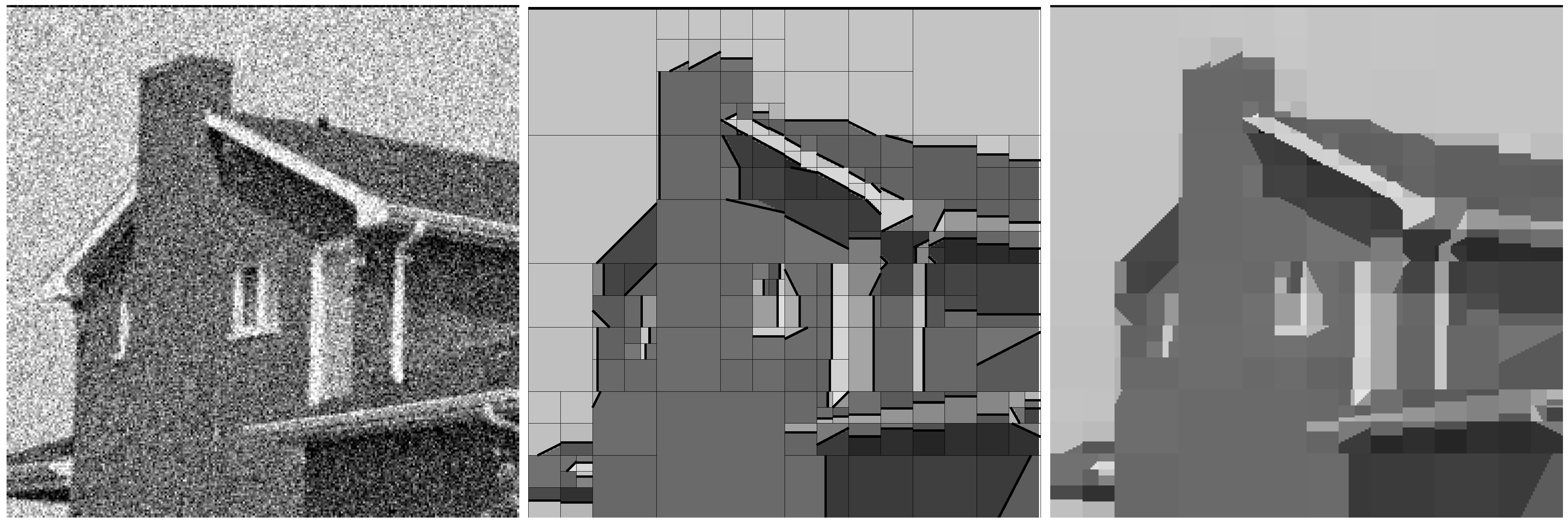Figure 1 illustrates a typical wedgelet representation of a noisy image.

Figure 1. A noisy image (left) and (right) a fairly rough wedgelet representation for $n=256$; the (middle) picture also shows the boundaries of the smoothness regions.

Figure 1. A noisy image (left) and (right) a fairly rough wedgelet representation for $n=256$; the (middle) picture also shows the boundaries of the smoothness regions.

Consistency is a strong indication that an estimation procedure is meaningful. Moreover, it allows for structural insight, since a sequence of discrete estimation procedures is embedded into a common continuous setting and the quantitative behavior of estimators can be compared. It is frequently used as a substitute or approximation for missing or vague knowledge in the real finite sample situation. Plainly, one must be aware of various shortcomings and should not rely on asymptotics in case of a small sample size. Nevertheless, consistency is a broadly accepted justification of statistical methods. Convergence rates are of particular importance, since they indicate the quality of discrete estimates or approximations and allow for comparison of different methods.

Observations or data will be governed by a simple regression model with additive white noise: Let $S^n={\{1,\dots ,n\}}^d$ be a finite discrete signal domain, interpreted as the discretization of the continuous domain, $S^{\infty }={[0,1)}^d$. Data, $y={\left(y_s\right)}_{s\in S^n}$, are available for the discrete domains and generated by the model:

$$Y_s^n={\overline{f}}_s^n+{\xi }_s^n,n\in \mathbb{N},s\in S^n$$

(1)

where ${({\overline{f}}_s^n)}_{s\in S^n}$ is a discretization of an original or “true” signal, f, on $S^{\infty }$ and ${\left({\xi }_s^n\right)}_{s\in S^n}$ is white sub-Gaussian noise.

The present approach is based on a partitioning of the discrete signal domain into regions on each of which a smooth approximation of noisy data is performed. The choice of a particular partition is obtained by a complexity penalized least squares estimation, dependent on the data. Between the regions, sharp breaks of intensity may happen, which allow for edge-preserving piecewise smoothing. In one dimension, a natural way to model jumps in signals is to consider piecewise regular functions. This naturally leads to representations based on partitions consisting of intervals. The number of intervals on a discrete line of length, n, is of the polynomial order, $n^2$.

In more dimensions, however, the definition of elementary fragments is much more involved. For example, in a discrete square of side-length, n, the number of all subregions is of the exponential order $2^{n^2}$. When dealing with images, one of the difficulties consists in constructing reduced sets of fragments, which, at the same time, take into account the geometry of images and lead to computationally feasible algorithms for the computation of estimators.

The estimators adopted here are minimal points of complexity penalized least squares functionals: If $y={\left(y_s\right)}_{s\in S^n}$ is a sample and $x={\left(x_s\right)}_{s\in S^n}$ a tentative representation of y, the functional:

$$H^n(x,y)=\gamma \left|𝒫\left(x\right)\right|+\sum _{s\in S^n}{(y_s-x_s)}^2$$

(2)

has to be minimized in x given y; the penalty, $\left|𝒫\right(x\left)\right|$, is the number of subdomains into which the entire domain is divided and on which x is smooth in a sense to be made precise by the choice of suitable function spaces (see Section 2.1 and Section 5); γ is a parameter that reflects the tradeoff between the quadratic error and the size of the partition.

Due to the non-convexity of the $L^0$-type penalty, one has to solve hard optimization problems in general. If all possible partitions of the signal domain are admitted, such optimization problems are not computationally feasible. A popular attempt to circumvent this nuisance is simulated annealing; see, for instance, the seminal paper [1]. This paper had a considerable impact on imaging; the authors transferred models from statistical physics to image analysis as prior distributions in the framework of Bayesian statistics. This approach was intimately connected with Markov Chain Monte Carlo methods, like Metropolis Sampling and Simulated Annealing [2].

On the other hand, transferring spatial complexity to time complexity, like in such metaheuristics, does not remove the basic problem; it rather transforms it. Such algorithms are not guaranteed to find the optimum or even a satisfactory near-optimal solution [2], Section 6.2. All metaheuristics will eventually encounter problems on which they perform poorly.

Moreover, if the number of partitions grows, at least, exponentially, it is difficult to derive useful uniform bounds on the projections of noise onto the subspaces induced by the partitions. Reducing the search space drastically allows the designing of exact and fast algorithms. Such a reduction basically amounts to restrictions on admissible partitions of the signal domain. There are various suggestions, some of them mentioned initially.

In one dimension, regression onto piecewise constant functions was proposed by the legendary [3] who called respective representations regressograms. The Functional (2) is by some (including the authors) referred to as the Potts functional. It was introduced in [4] as a generalization of the well-known Ising model [5] from statistical physics from two or more spins. It was suggested by [6] and penalizes the length of contours between regions of constant spins. In fact, in one dimension, a partition, $𝒫$, into, say, k intervals on which the signal is constant admits $k-1$ jumps and, therefore, has contour-length, $k-1$.

The one-dimensional Potts model for signals was studied in detail in a series of theses and articles; see [7,8,9,10,11,12,13,14] Consistency was first addressed in [10] and, later on, exhaustively treated in [15,16]. Partitions there consist of intervals. Our study of the multi-dimensional case started with the thesis [8]; see also [17].

In two or more dimensions, the model (2) differs substantially from the classical Potts model. The latter penalizes the length of contours—locations of intensity breaks—whereas (2) penalizes the number of regions. This allows, for instance, good performance on filamentous structures, albeit having long borders compared to their area.

Let us give an informal introduction into the setting. The aim is to estimate a function, f, on the d-dimensional unit cube, $S^{\infty }={[0,1)}^d$, from discrete data. To this end, $S^{\infty }$ and f are discretized to cubic grids, $S^n={\{1,\dots ,n\}}^d$, $n\in \mathbb{N}$, and functions, ${\overline{f}}^n$, on $S^n$. For each n, data, $y_s^n$, $s\in S^n$, is available, i.e., noisy observations of the ${\overline{f}}_s^n$.

In this paper, we prove almost sure convergence of the quadratic error associated with complexity penalized least squares estimators ${\widehat{f}}^n\left(y\right)$, which are minimal points of functionals of the form (2) (see Section 2.2). Note that the partition, $\mathcal{P}$, is chosen among a suitable class of admissible partitions. Moreover, we derive almost sure convergence rates of quadratic errors, whenever a decay rate of the approximation errors is assumed in addition.

We are faced with three kinds of error: The error caused by noise, the approximation and the discretization error. Noise is essentially controlled regardless of the specific form of f. For the approximation and the discretization error, special assumptions on the function classes in question are needed.

The results presented here are closely related to—but differ from—those obtained by the classical model selection theory developed, for instance, in [18,19]. In fact, classical model selection works within the minimax setting, where the quadratic risk, $\mathbb{E}(\parallel {\widehat{f}}^n\left(\omega \right)-{\overline{f}}^n{\parallel }^2)$, is controlled. Let us stress that neither of both results directly implies the other.

Due to the approximation error term, there are deep connections to approximation theory. In particular, when dealing with piecewise regular images, non-linear approximation rates obtained by wavelet shrinkage methods are known to be suboptimal, as discussed in [20,21]. In the last decade, the challenging problem to improve upon wavelets has been addressed in very different directions.

The search for a good paradigm for detecting and representing curvilinear discontinuities of bivariate functions remains a fundamental issue in image analysis. Ideally, an efficient representation should use atomic decompositions, which are local in space (like wavelets), but also possess appropriate directional properties (unlike wavelets). One of the most prominent examples is given by curvelet representations, which are based on multiscale directional filtering combined with anisotropic scaling. [22] proved that thresholding of curvelet coefficients provides estimators, which yield the minimax convergence rate up to a logarithmic factor for piecewise ${𝒞}^2$ functions with ${𝒞}^2$ boundaries. Another interesting representation is given by bandelets, as proposed in [23]. Bandelets are based on optimal local warping in the image domain relative to the geometrical flow, and [24] proved, also, the optimality of the minimax convergence rates of their bandelet-based estimator, for a larger class of functions, including piecewise ${𝒞}^{\alpha }$ functions with ${𝒞}^{\alpha }$ boundaries.

In Section 5, we apply the abstract framework proposed in Section 4 to bidimensional examples that rely on explicit geometrical constructions: In particular, the corresponding approaches are aimed at avoiding the pseudo-Gibbs artifacts produced by the above methods.

Wedgelet partitions were introduced by [21] and belong to the class of shape-preserving image segmentation methods. The decompositions are based on local polynomial approximation on some adaptively selected leaves of a quadtree structure. The use of a suitable data structure allowed for the development of fast algorithms for wedgelet decomposition; see [17].

An alternative is provided by anisotropic Delaunay triangulations, which have been proposed in the context of image compression in [25]. The flexible design of the representing system allows for a particularly fine selection of triangles fitting the anisotropic geometrical features of images. In contrast to curvelets, such representations preserve the advantage of wavelets and are still able to approximate point singularities optimally; see [26].

Both wedgelet representations and anisotropic Delaunay triangulations lead to optimal non-linear approximation rates for some classes of piecewise smooth functions. Note that the classes of (generalized horizon) functions considered in this paper contain and are larger than the above mentioned horizon functions (or boundary fragments). For a brief discussion on the generalization to more general piecewise regular functions, see Section 6. In the present paper, we use this optimality to derive convergence rates of the estimators. We prove almost sure consistency rates for function classes where the piecewise regularity is controlled by a parameter, α. More precisely, for these classes, we obtain that, for almost each ω:

$$\parallel {\widehat{f}}^n\left(\omega \right)-f\parallel =O({\epsilon }_n^{2\alpha /(\alpha +1)}log\left({\epsilon }_n\right)),{\epsilon }_n={\sigma }^2/n^d$$

(3)

where ${\sigma }^2$ is the variance of noise.

In the minimax setting, decay rates similar to those in (3) are known to be optimal for the respective function classes. Note that, using slightly modified penalties, which are not merely proportional to the number of pieces, [27] were able to show that optimal minimax rates may be achieved, optimally meaning that the rates are of the same order as in (3), but without the log factor. In the present paper, in contrast to [27], we control the almost sure convergence instead of the $L^2$-risk. Moreover, we explicitly restrict our attention to the classical penalty given by the number of pieces (or, equivalently, the dimension of the model) as in (2), noting that this is strongly connected to the sparse ansatz, which is currently popular in the signal community. We refer to [28] for a comprehensive review on sparsity. The generalization of the results in the present paper to other penalties is straightforward, but would be rather technical and, thus, might obscure the main ideas.

We address, first, noise and its projections to the approximation spaces; see Section 3. In Section 4, we derive convergence rates in the general context. Finally, in Section 5, we illustrate the abstract results by specific applications. Dimension, 1, is included, thus generalizing the results from [15] to piecewise polynomial regression and piecewise Sobolev classes. Our two-dimensional examples, wedgelets and Delaunay triangulations both rely on a geometric and edge-preserving representation. Our main motivation is the optimal approximation properties of these methods, the key feature to apply the previous framework being an appropriate discretization of these schemes.

2. The Setting

In this section, we introduce the formal framework for piecewise smooth representations, the regression model for data and the estimation procedure.

2.1. Regression and Segmentations

Image domains will generically be denoted by S. We choose $S^{\infty }={[0,1)}^d$, $d\in \mathbb{N}$, as the continuous and $S^n={\{1,\dots ,n\}}^d$ as the generic discrete image domain. Let $f\in L^2\left(S^{\infty }\right)$ represent the “true” image, which has to be reconstructed from noisy discrete data. For the latter, we adopt a simple linear regression model of the form:

$$Y_s^n={\overline{f}}_s^n+{\xi }_s^n,n\in \mathbb{N},s\in S^n$$

(4)

The noise variables, ${\xi }_s^n$, in the regression model are random variables on a common probability space $(\Omega ,ℱ,\mathbb{P})$. $\overline{f^n}={\left({\overline{f^n}}_s\right)}_{s\in S^n}$ is a discretization of f. To be definite, divide $S^{\infty }$ into $n^d$ semi-open cubes:

$$I_{i_1,\dots ,i_d}^n=\prod _{1\le j\le d}[(i_j-1)/n,i_j/n),1\le i_j\le n$$

of volume $1/n^d$ and for $g\in L^2\left(S^{\infty }\right)$ take local means

$${\overline{g}}_s^n=n^d{\int }_{I_s}g\left(u\right)du,s\in S^n$$

This specifies maps, ${\delta }^n$, from $L^2\left(S^{\infty }\right)$ to ${\mathbb{R}}^{S^n}$ by:

$${\delta }^{n}g={\left({\overline{g}}_s^n\right)}_{s\in S^n}$$

(5)

Conversely, embeddings of ${\mathbb{R}}^{S^n}$ into $L^2\left(S^{\infty }\right)$ are defined by:

$$z={\left(z_s\right)}_{s\in S^n}⟼{\iota }^{n}z=\sum _{s\in S^n}{z}_s{1}_{I_s}$$

(6)

As an aid to memory, keep the following chain of maps in mind:

$$L^2\left(S^{\infty }\right)\stackrel{{\delta }^n}{⟶}{\mathbb{R}}^{S^n}\stackrel{{\iota }^n}{⟶}{L}^2\left(S^{\infty }\right)$$

In the absence of noise, the discrete approximations of f are the functions, ${\iota }^n{\overline{f}}^n={\iota }^n{\delta }^{n}f$, which approximate f more and more precisely as n tends to infinity. Thus, a crucial issue will be to control noise. In fact, the function, ${\iota }^n{\delta }^{n}f={\iota }^n{\overline{f}}^n$, is the conditional expectation of f with regard to the (σ)-algebra ${𝒜}^n$ generated by the cubes, $I_s^n$, and convergence can be seen by a martingale argument.

We are dealing with estimates of f or, rather, of ${\overline{f}}^n$ on each level, n. An image domain, S, will be partitioned by the method into sets, on which the future representations are members of initially chosen spaces of smooth functions. To keep control, we choose a class, $ℛ\subset 2^S$, of admissible fragments, and later on, these will be rectangles, wedges or triangles. A subset, $𝒫\subset 2^S$, is a partition if (a) the elements in $𝒫$ are mutually disjoint and (b) S is the union of all $P\in 𝒫$. In the following, $\mathfrak{P}$ is a fixed subset of partitions, $𝒫$, such that $𝒫\subset ℛ$. We call elements of $\mathfrak{P}$ admissible partitions.

For each fragment, $P\in ℛ$, we choose a finite dimensional linear space, ${ℱ}_P$, of real functions on S, which vanish off P. Examples are spaces of constant functions or polynomials of higher degree, set to 0 outside P. If $𝒫\in \mathfrak{P}$ and $f_{𝒫}={\left(f_P\right)}_{P\in 𝒫}$ is a family of such functions, we also denote by $f_{𝒫}$ the function defined on all of S and whose restriction to P is equal to $f_P$ for each $P\in 𝒫$. The pair, $(𝒫,f_{𝒫})$, is a segmentation, and each element $(P,f_P)$ is a segment. For each partition, $𝒫$, define the linear space, ${\oplus }_{P\in 𝒫}{ℱ}_P$. A family of segmentations is called a segmentation class. In particular, for a given set of functions, ${ℱ}_P,P\in 𝒫$, we let:

$$\mathfrak{S}\left(\mathfrak{P}\right):=\left\{(𝒫,f):\mathcal{P}\in \mathfrak{P},f\in {ℱ}_{𝒫}\right\}$$

with partitions in $\mathfrak{P}$ and functions whose restrictions to $P\in 𝒫$ are in ${ℱ}_P$. We will also use the notation, ${\mathfrak{S}}^n$, for the discrete equivalent of $\mathfrak{S}$ obtained from discrete partitions, ${𝒫}^n$.

2.2. Complexity Penalized Least Squares Estimation

We want to produce appropriate discrete representations or estimates of the underlying function, f, on the basis of random data, Y, from the regression model (4). We are watching out for a segmentation that is in proper balance between fidelity to data and complexity.

We decide in advance on a class, ${\mathfrak{S}}^n$, of (admissible) discrete segmentations, which should contain the desired representations. The segmentations, given data, $Y^n$, are scored by the functional:

$$H_{\gamma }^n:{\mathfrak{S}}^n\times {\mathbb{R}}^{S^n}⟶\mathbb{R},H_{\gamma }^n\left((𝒫,f_{𝒫}),Y^n\right)=\gamma \left|𝒫\right|+\parallel f_{𝒫}-Y^n{\parallel }^2$$

(7)

with $\gamma \ge 0$ and $\left|𝒫\right|$ being the cardinality of $𝒫$. The symbol, $\parallel ·\parallel$, denotes the ${\ell }^2$-norm on ${\mathbb{R}}^{S^n}$. The last term measures fidelity to data. The other term is a rough measure of overall smoothness. As estimators for f given data, Y, we choose minimizers: $(\widehat{{𝒫}^n},{\widehat{f}}^n)$ of (7). Note that both $\widehat{{𝒫}^n}$ and ${\widehat{f}}^n$ are random since $Y^n$ is random.

The definition makes sense, since minimal points of (7) always exist. This can be easily verified by the reduction principle, which relies on the decomposition:

$$\underset{𝒫\in {\mathfrak{P}}^n,f_{𝒫}\in {ℱ}_{𝒫}}{min}{H}_{\gamma }^n((𝒫,f_{𝒫}),Y)=\underset{𝒫\in {\mathfrak{P}}^n}{min}\left(\gamma \left|𝒫\right|+\underset{f_{𝒫}\in {ℱ}_{𝒫}}{min}{\parallel f_{𝒫}-Y\parallel }^2\right)$$

Given $𝒫$, the inner minimization problem has as a unique solution the orthogonal projection, ${\widehat{f}}_{𝒫}^n$, of Y onto ${\oplus }_{P\in 𝒫}{ℱ}_P$. The outer minimization problem is finite, and hence, a minimum of (7) exists. Let us pick one of the minimal points, ${\widehat{f}}^n$.

The reduction principle connects complexity penalized least squares to model choice techniques. The right side can be interpreted as a criterion for the choice of a partition, $\mathcal{P}$. The chosen partition determines the linear space, ${\mathcal{F}}_{\mathcal{P}}$, which is a linear model for data. Based on this model, the estimate is finally derived.

3. Noise and Its Projections

For consistency, resolutions at infinitely many levels are considered simultaneously. Frequently, segmentations are not defined for all $n\in \mathbb{N}$, but only for a cofinal subset of $\mathbb{N}$. Typical examples are all dyadic quad-tree partitions or dyadic wedgelet segmentations, where only indices of the form, $n=2^p$, appear. Therefore, we adopt the following convention:

The symbol, $\mathbb{M}$, denotes any infinite subset of $\mathbb{N}$ endowed with the natural order, ≤. $(\mathbb{M},\le )$ is a totally ordered set, and we may consider nets, ${\left(x_n\right)}_{n\in \mathbb{M}}$. For example, $x_n\to x$, $n\in \mathbb{M}$, means that $x_n$ convergences to x along $\mathbb{M}$. We deal similarly with notions, like lim sup etc. Plainly, we might resort to subsequences instead, but this would cause a change of indices, which is notationally inconvenient.

3.1. Sub-Gaussian Noise and a Tail Estimate

We introduce now the main hypotheses on noise accompanied by a brief discussion. The core of the arguments in later sections is the tail Estimate Equation (9) below.

As Theorem 2 will show, the appropriate framework are sub-Gaussian random variables. A random variable, ξ, enjoys this property if one of the following conditions is fulfilled:

Theorem 1 

The following two conditions on a random variable ξ are equivalent:

(a)

There is $a\in \mathbb{R}$, such that:

$$\mathbb{E}(exp\left(t\xi \right))\le exp(a^2{t}^2/2)foreveryt>0$$

(8)

(b)

ξ is centered and majorized in distribution by some centered Gaussian variable, η, i.e.:

$$thereis{c}_0\ge 0\text{,}suchthat\mathbb{P}\left(\right|\xi |\ge c)\le \mathbb{P}\left(\right|\eta |\ge c)\text{,}forallc>c_0$$

This and most other facts about sub-Gaussian variables quoted in this paper are verified in the first few sections of the monograph, [29]; one may also consult [30], Section 3.4.

The definition in (a) was given in the celebrated paper [31], which uses the term generalized Gaussian variables. The closely related concept of semi-Gaussian variables, which requires symmetry of ξ, seems to go back to [32].

The class of all sub-Gaussian random variables living on a common probability space, $(\Omega ,𝒜,\mathbb{P})$, is denoted by $\text{Sub}\left(\Omega \right)$. The sub-Gaussian standard is the number,

$$\tau \left(\eta \right)=inf\{a\ge 0:a\text{is}\text{feasible}\text{in}(8\left)\right\}$$

The infimum is attained and, hence, is a minimum. $\text{Sub}\left(\Omega \right)$ is a linear space, τ is a norm on $\text{Sub}\left(\Omega \right)$ if variables differing on a null-set only are identified. Equipped with the norm, τ, $\text{Sub}\left(\Omega \right)$ is a Banach space. It is important to note that $\text{Sub}\left(\Omega \right)$ is strictly contained in all spaces, $L_0^p\left(\Omega \right)$, $p\ge 1$, the spaces of all centered variables with finite $pth$ ordered absolute moments.

Remark 1 

The most prominent sub-Gaussians are centered Gaussian variables, η, with standard deviation, σ, and $\tau \left(\eta \right)=\sigma$. For them, Inequality (8) is an equality with $a=\sigma$. The specific characteristic of sub-Gaussian variables are tails lighter than those of Gaussians, as expressed in (b) of Theorem 1.

The following theorem is essential in the present context:

Theorem 2 

For each $n\in \mathbb{M}$, suppose that the variables, ${\xi }_s^n$, $s\in S^n$, are independent. Then:

(a)

Suppose that there is a real number, $\beta >0$, such that for each $n\in \mathbb{M}$ and real numbers, ${\mu }_s$, $s\in S^n$, and each $c\in {\mathbb{R}}_{+}$, the inequality:

$$\mathbb{P}\left(\left|\sum _{s\in S_n}{\mu }_s{\xi }_s^n\right|\ge c\right)\le 2·exp\left({\displaystyle -\frac{c^2}{\beta {\sum }_{s\in S_n}{\mu }_s^2}}\right)$$

(9)

holds. Then, all variables ${\xi }_s^n$ are sub-Gaussian with a common scale factor, β.

(b)

Let all variables, ${\xi }_s^n$, be sub-Gaussian. Suppose further that:

$$\beta =2·sup\{{\tau }^2\left({\xi }_s^n\right):n\in \mathbb{M},s\in S^n\}<\infty$$

(10)

Then, (a) is fulfilled with this factor, β.

This is probably folklore, and we skip the proof. A detailed proof can be found in the extended version [33].

Remark 2 

For white Gaussian noise, one has $\tau \left({\xi }_s^n\right)=\sigma$ and, hence, $\beta =2{\sigma }^2$.

3.2. Noise Projections

In this section, we quantify projections of noise. Choose for each $n\in \mathbb{M}$ a class, ${ℛ}^n\subset {\mathfrak{P}}^n\times 2^{S^n}$, of admissible segments over $S^n$ and a set, ${\mathfrak{P}}^n$, of admissible partitions. As previously, for each $P\in {ℛ}^n$, a linear function space, ${ℱ}_P$, is given. We shall denote the orthogonal $L^2$-projection onto the linear space, ${\oplus }_{P\in 𝒫}{F}_{𝒫}$, by ${\pi }_{𝒫}$.

The following result provides almost sure $L^2$-estimates for the projections of noise to these spaces, as there are more and more admissible segments.

Proposition 1 

Suppose that $\dim {ℱ}_P\le D$ for all $n\in \mathbb{M}$ and each $P\in {ℛ}^n$. Assume in addition that there is a number, $M>0$, such that for some $\kappa >0$:

$$\left|{ℛ}^n\right|\ge M·n^{\kappa }eventually$$

Let $\gamma >0$. Then, we have:

$$\begin{array}{ccc}& & \mathbb{P}\left(thereis{𝒫}^n\in {\mathfrak{P}}^n|\parallel {\pi }_{{𝒫}^n}{\xi }^n{\parallel }^2>(\gamma /\kappa +1)\beta D\left|{𝒫}^n\right|ln\left({ℛ}^n\right)\right)\hfill \\ & \le & 2D{M}^{-\gamma /\kappa }{n}^{-\gamma }\hfill \end{array}$$

(11)

Moreover, for $\gamma >1$ and for almost all ω, there is $n_0\left(\omega \right)\in \mathbb{M}$, such that for $n\ge n_0$:

$$andforall{𝒫}^n\in {\mathfrak{P}}^n,{∥{\pi }_{{𝒫}^n}{\xi }^n\left(\omega \right)∥}^2\le (\gamma /\kappa +1)\beta D|{𝒫}^n|ln(|{ℛ}^n\left|\right)$$

(12)

This will be proven at a more abstract level. No structure of the finite sets, $S^n$, is required. Nevertheless, we adopt all definitions from Section 1, mutatis mutandis. All Euclidean spaces, ${\mathbb{R}}^k$, will be endowed with their natural inner products, $\langle ·,·\rangle$, and respective norms. The projection onto the linear subspace $\mathscr{H}$ will be denoted by ${\pi }_{\mathscr{H}}$.

Theorem 3 

Suppose that the noise variables, ${\xi }_s^n$, fulfill (9) accordingly. Consider finite nonempty collections, ${\mathfrak{H}}^n$, of linear subspaces in ${\mathbb{R}}^{S^n}$, and assume that the dimensions of all subspaces, $\mathscr{H}\in {\mathfrak{H}}^n$, $n\in \mathbb{M}$, are uniformly bounded by some number, $D\in \mathbb{N}$. Assume in addition that there is a number, $M>0$, such that for some $\kappa >0$:

$$\left|{\mathfrak{H}}^n\right|\ge M·n^{\kappa }eventually$$

Let $\gamma >0$. Then, we have

$$\mathbb{P}\left(thereis\mathscr{H}\in {\mathfrak{H}}^n|\parallel {\pi }_{\mathscr{H}}{\xi }^n{\parallel }^2\ge (\gamma /\kappa +1)\beta Dln\left({\mathfrak{H}}^n\right)\right)\le 2D{M}^{-\gamma /\kappa }{n}^{-\gamma }$$

Note that $\parallel ·\parallel$ is the Euclidean norm in the spaces, ${\mathbb{R}}^{S^n}$, since each ${\xi }^n\left(\omega \right)$ is simply a vector. The assumption in the theorem can be reformulated as $|{\mathfrak{H}}^n{|}^{-1}=O\left(n^{-\kappa }\right)$.

Proof. 

Choose $n\in \mathbb{M}$ and $\mathscr{H}\in {\mathfrak{H}}^n$ with $dim\mathscr{H}=d_n$. Let $e_i$, $1\le i\le d_n$ be some orthonormal basis of $\mathscr{H}$. Observe that for any real number, $c>0$:

$$\sum _{i=1}^{d_n}|\langle {\xi }^n\left(\omega \right),e_i\rangle {|}^2>c^{2}ln\left|{\mathfrak{H}}^n\right|$$

implies that:

$$|\langle {\xi }^n\left(\omega \right),e_i\rangle {|}^2>\frac{c^2}{d_n}ln\left|{\mathfrak{H}}^n\right|\text{for}\text{at}\text{least}\text{one}i=1,\dots ,d_n$$

We derive a series of inequalities:

$$\begin{array}{ccc}& & \mathbb{P}\left({∥{\pi }_H{\xi }^n∥}^2>c^{2}ln\left|{\mathfrak{H}}^n\right|\right)=\mathbb{P}\left(\sum _{i=1}^{d_n}|\langle {\xi }^n,e_i\rangle {|}^2>c^{2}ln\left|{\mathfrak{H}}^n\right|\right)\hfill \\ & \le & \mathbb{P}\left(\bigcup _{i=1}^{d_n}\left\{\right|\langle {\xi }^n,e_i\rangle {|}^2>\frac{c^2}{d_n}ln|{\mathfrak{H}}^n\left|\right\}\right)\le \sum _{i=1}^{d_n}\mathbb{P}\left(|\langle {\xi }^n,e_i\rangle {|}^2>\frac{c^2}{d_n}ln|{\mathfrak{H}}^n|\right)\hfill \\ & \le & \sum _{i=1}^{d_n}\mathbb{P}\left(\left|\sum _{s\in S^n}{\xi }_s^n{e}_{i,s}\right|>c{\left(ln|{\mathfrak{H}}^n|/d_n\right)}^{1/2}\right)\hfill \end{array}$$

where the first inequality follows from the introductory implication. By (9), we may continue with:

$$\le 2·d_{n}exp\left(\frac{-c^{2}ln|{\mathfrak{H}}^n|}{\beta d_n{\sum }_{s\in S^n}{e}_{i,s}^2}\right)\le 2·D·{\left|{\mathfrak{H}}^n\right|}^{\frac{-c^2}{\beta D}}$$

This implies that:

$$\begin{array}{ccc}& & \mathbb{P}\left(\exists \mathscr{H}\in {\mathfrak{H}}^n|\parallel {\pi }_{\mathcal{H}}{\xi }^n{\parallel }^2\ge c^{2}ln\left({\mathfrak{h}}^n\right)\right)\le \sum _{\mathscr{H}\in {\mathfrak{H}}^n}\mathbb{P}\left({∥{\pi }_{\mathscr{H}}{\xi }^n∥}^2>c^{2}ln\left|{\mathfrak{H}}^n\right|\right)\hfill \\ & \le & 2D\sum _{\mathscr{H}\in {\mathfrak{H}}^n}|{\mathfrak{H}}^n{|}^{\frac{-c^2}{\beta D}}\le 2D|{\mathfrak{H}}^n\left|\right|{\mathfrak{H}}^n{|}^{\frac{-c^2}{\beta D}}\hfill \\ & \le & 2D{\left(\frac{1}{M}·n^{-\kappa }\right)}^{\frac{c^2}{\beta D}-1}=2D·M^{1-c^2/\left(\beta D\right)}{n}^{-\kappa (\frac{c^2}{\beta D}-1)}\hfill \end{array}$$

Let $\gamma >0$. For $c^2=(\gamma /\kappa +1)\beta D$:

$$\mathbb{P}\left(\exists \mathscr{H}\in {\mathfrak{H}}^n|\parallel {\pi }_{\mathcal{H}}{\xi }^n{\parallel }^2\ge (\gamma /\kappa +1)\beta Dln\left({\mathfrak{H}}^n\right)\right)\le 2D{M}^{-\gamma /\kappa }{n}^{-\gamma }$$

and the assertion is proven. $\square$

Now, let us prove Proposition 1:

Proof of Proposition 1. 

We apply Theorem 3 to the collections, ${\mathfrak{H}}^n=\{{ℱ}_R:R\in {ℛ}^n\}$. Then, $|{\mathfrak{H}}^n|=|{ℛ}^n|$. Since for each ${𝒫}^n\in {\mathfrak{P}}^n$, the spaces, ${ℱ}_P$, $P\in {𝒫}^n$, are mutually orthogonal, one has for $z\in {\mathbb{R}}^{S^n}$ that:

$$\parallel {\pi }_{{𝒫}^n}{z\parallel }^2=\sum _{P\in {𝒫}^n}{\parallel {\pi }_{{ℱ}_P^n}z\parallel }^2$$

In particular, we have:

$$\begin{array}{cc}& \mathbb{P}\left(\sum _{P\in {𝒫}^n}\parallel {\pi }_{{ℱ}_P^n}{\parallel }^2>\left(\frac{\gamma }{\kappa }+1\right)\beta Dln\left({\mathfrak{H}}^n\right)\left|{𝒫}^n\right|\right)\\ & \le \mathbb{P}\left(\exists P\in {𝒫}^n|\parallel {\pi }_{{ℱ}_P^n}{\parallel }^2>\left(\frac{\gamma }{\kappa }+1\right)\beta Dln\left({\mathfrak{H}}^n\right)\left|{𝒫}^n\right|\right)\end{array}$$

Applying Theorem 3 to the latter inequality Proves (11). Moreover, for $\gamma <1$, we observe that the right hand side of (11) has a finite sum over n. Thus, the Borel-Cantelli lemma yields:

$$\begin{array}{ccc}& & \mathbb{P}\left(\parallel {\pi }_{{𝒫}^n}{\xi }^n\parallel >\left(\frac{\gamma }{\kappa }+1\right)\beta D|{𝒫}^n|ln|{ℛ}_n|\right.\hfill \\ & & \left.\text{for}\text{finitely}\text{many}(n,{𝒫}^n)\text{with}{𝒫}^n\in {\mathfrak{P}}^n\right)=1\hfill \end{array}$$

This implies (12). $\square$

Let us finally illustrate the above concept in the classical case of Gaussian white noise.

Remark 3 

Continuing from Remark 2, we illustrate the behavior of the lower bound for the constant, C, in Proposition 1 and Theorem 3, in the case of white Gaussian noise and polynomially growing number of fragments, i.e., $|{ℛ}^n|$ is asymptotically equivalent to $n^{\kappa }$. In this case, the estimate for the norm of noise projections takes the form, for almost all ω and for $n\ge n_0$:

$$\begin{array}{ccc}\hfill \parallel {\pi }_{{𝒫}^n}{\xi }^n{\left(\omega \right)\parallel }^2& \le & \left(\frac{1}{\kappa }+1\right)\kappa 2{\sigma }^{2}D|{𝒫}^n|lnn=(1+\kappa )2{\sigma }^{2}D\left|{𝒫}^n\right|lnn\hfill \end{array}$$

This underlines the dependency between the noise projections, the number of fragments, the noise variance, the dimension of the regression spaces and the size of the partitions.

3.3. Discrete and Continuous Functionals

We want to approximate functions, f, on the continuous domain, $S^{\infty }={[0,1)}^d$, by estimates on discrete finite grids, $S^n$. The connections between the two settings are provided by the maps, ${\iota }^n$ and ${\delta }^n$, introduced in (5) and (6). Note first that:

$$\langle {\iota }^{n}x,{\iota }^{n}y\rangle =\langle x,y\rangle /|S^n|\text{and}\parallel {\iota }^n{x\parallel }^2={\parallel x\parallel }^2/\left|S^n\right|\text{for}x,y\in {\mathbb{R}}^{S^n}$$

(13)

where the inner product and norm on the respective left-hand sides are those on $L^2\left(S^{\infty }\right)$, and on the right-hand sides, one has the Euclidean inner product and norm. Furthermore, one needs appropriate versions of the Functionals (7). Let now ${\mathfrak{S}}^n$ be segmentation classes on the domains, $S^n$, and $\mathfrak{S}\supset {\iota }^n{\mathfrak{S}}^n$ a segmentation class on $S^{\infty }$. Set:

$$\begin{array}{ccc}\hfill H_{\gamma }^n:{\mathbb{R}}^{S^n}\times {\mathfrak{S}}^n,H_{\gamma }^n(z,({𝒫}^n,g_{{𝒫}^n}^n))& =& \gamma |{𝒫}^n|+\parallel z-g_{{𝒫}^n}{\parallel }^2/\left|S^n\right|\hfill \\ \hfill {\tilde{H}}_{\gamma }^n:L^2\left(S^{\infty }\right)\times \mathfrak{S},{\tilde{H}}_{\gamma }^n(f,(𝒫,g_{𝒫}))& =& \left\{\begin{array}{cc}\gamma \left|𝒫\right|+\parallel f-g_{𝒫}{\parallel }^2& \text{if}(𝒫,g_{𝒫})\in {\iota }^n{\mathfrak{S}}^n\hfill \\ \infty & \text{otherwise}\hfill \end{array}\right.\hfill \end{array}$$

The two functionals are compatible.

Proposition 2 

Let $n\in \mathbb{M}$ and $({𝒫}^n,g_{{𝒫}^n})\in {\mathfrak{S}}^n$ and $z^n\in {\mathbb{R}}^{S^n}$. Then,

$$H_{\gamma }^n(z^n,{({𝒫}^n,g_{{𝒫}^n})}^n)={\tilde{H}}_{\gamma }^n({\iota }^n{z}^n,{\iota }^n({𝒫}^n,g_{{𝒫}^n}^n))$$

If, moreover, $f\in L^2\left(S^{\infty }\right)$ then:

$$({𝒫}^n,g_{{𝒫}^n}^n)\in \mathrm{argmin}{H}_{\gamma }^n({\delta }^{n}f,·)⟺{\iota }^n({𝒫}^n,g_{{𝒫}^n}^n)\in \mathrm{argmin}{\tilde{H}}_{\gamma }^n(f,·)$$

Proof. 

The identity is an immediate consequence of (13). Hence, let us turn to the equivalence of minimal points. The key is a suitable decomposition of the functional, ${\tilde{H}}_{\gamma }^n(f,·)$. The map, ${\iota }^n{\delta }^n$, is the orthogonal projection of $L^2\left(S^{\infty }\right)$ onto the linear space, ${\mathscr{H}}^n=\mathrm{span}\left\{1_{I_{ij}:1\le i,j\le n}\right\}$, and for any $(𝒫,h)\in {\iota }^n{\mathfrak{S}}^n$, the function, h, is in ${\mathscr{H}}^n$. Hence:

$${\parallel f-h\parallel }^2+\gamma \left|𝒫\right|=\parallel f-{\iota }^n{\delta }^n{f\parallel }^2+\parallel {\iota }^n{\delta }^n{f-h\parallel }^2+\gamma \left|𝒫\right|$$

The quantity, $\parallel f-{\iota }^n{\delta }^n{f\parallel }^2$, does not depend on $(𝒫,h)$. Therefore, a pair, $(𝒫,h)$, minimizes

$$\parallel f-{\iota }^n{\delta }^n{f\parallel }^2+\parallel {\iota }^n{\delta }^n{f-h\parallel }^2+\gamma \left|𝒫\right|$$

if and only if it minimizes

$$\parallel {\iota }^n{\delta }^n{f-h\parallel }^2+\gamma \left|𝒫\right|={\tilde{H}}_{\gamma }^n({\iota }^n{\delta }^{n}f,{\iota }^n(𝒫,h))$$

Setting $z^n={\delta }^{n}f$ in (2), this completes the proof. $\square$

3.4. Upper Bound for Projective Segmentation Classes

We compute an upper bound for the estimation error in a special setting: choose in advance a finite dimensional linear subspace, $𝒢$ of $L^2\left(S^{\infty }\right)$. Discretization induces linear spaces, ${\delta }^n𝒢=\{{\delta }^{n}f:f\in 𝒢\}$ and ${𝒢}_P^n=\{1_P·g:g\in {\delta }^n𝒢\}$, for any $P\subset S^n$, of functions on $S^n$. Let further for each $n\in \mathbb{M}$, a set, ${ℛ}^n$, of admissible fragments and a family, ${\mathfrak{P}}^n$, of partitions with fragments in ${ℛ}^n$ be given. Set ${\mathfrak{G}}^n:=\left\{{𝒢}_{𝒫}:𝒫\in {\mathfrak{P}}^n\right\}$. The induced segmentation class,

$${\mathfrak{S}}^n({\mathfrak{P}}^n,{\mathfrak{G}}^n)=\left\{({\mathfrak{P}}^n,f):\exists 𝒫\in {\mathfrak{P}}^n,f\in {𝒢}_{𝒫}\right\}$$

will be called projective $𝒢$-segmentation class at stage, n.

The following inequality is at the heart of later arguments since it controls the distance between the discrete M-estimates and the “true” signal. Note that this result is also central in the derivation of the results of the model selection theory.

Lemma 1 

Let for $n\in \mathbb{M}$ a $𝒢$-projective segmentation class, ${\mathfrak{S}}^n$, over $S^n$ be given and choose a signal, $f\in L^2\left(S^{\infty }\right)$, and a vector, ${\xi }^n\in {\mathbb{R}}^{S^n}$. Let further

$$({\widehat{𝒫}}^n,{\widehat{f}}^n)\in \underset{(𝒬,h)\in {\mathfrak{S}}^n}{\mathrm{argmin}}{H}_{\gamma }^n({\delta }^{n}f+{\xi }^n,(𝒬,h))$$

and $(𝒬,h)\in {\mathfrak{S}}^n$. Then,

$$\parallel {\iota }^n{\widehat{f}}^n{-f\parallel }^2\le 2\gamma \left(\right|𝒬|-|{\widehat{𝒫}}^n\left|\right)+3\parallel {\iota }^n{h-f\parallel }^2+\frac{16}{n^d}\left(\parallel {\pi }_{{\widehat{𝒫}}^n}{\xi }^n{\parallel }^2+{\parallel {\pi }_{𝒬}{\xi }^n\parallel }^2\right)$$

(14)

Proof. 

Since $({\widehat{𝒫}}^n,{\widehat{f}}^n)$ is a minimal point of $H_{\gamma }^n({\delta }^{n}f+{\xi }^n,·)$, the embedded segmentation, ${\iota }^n({\widehat{𝒫}}^n,{\widehat{f}}^n)$, is a minimal point of ${\tilde{H}}_{\gamma }^n(f+{\iota }^n{\xi }^n,·)$ by Proposition 2 and, hence:

$$\gamma |{\widehat{𝒫}}^n|+\parallel ({\iota }^n{\widehat{f}}^n-f)-{\iota }^n{\xi }^n{\parallel }^2\le \gamma \left|𝒬\right|+\parallel ({\iota }^{n}h-f)-{\iota }^n{\xi }^n{\parallel }^2$$

Expansion of squares yields that:

$$\begin{array}{ccc}& & \gamma |{\widehat{𝒫}}^n|+\parallel {\iota }^n{\widehat{f}}^n{-f\parallel }^2+2\langle {\iota }^n{\widehat{f}}^n-f,{\iota }^n{\xi }^n\rangle +{\parallel {\iota }^n{\xi }^n\parallel }^2\hfill \\ & \le & \gamma \left|𝒬\right|+\parallel {\iota }^n{h-f\parallel }^2+2\langle {\iota }^{n}h-f,{\iota }^n{\xi }^n\rangle +{\parallel {\iota }^n{\xi }^n\parallel }^2\hfill \end{array}$$

and hence:

$$\parallel {\iota }^n{\widehat{f}}^n{-f\parallel }^2\le \gamma \left(\right|𝒬|-|{\widehat{𝒫}}^n\left|\right)+\parallel {\iota }^n{h-f\parallel }^2+2\langle {\iota }^{n}h-{\iota }^n{\widehat{f}}^n,{\iota }^n{\xi }^n\rangle$$

(15)

By definition, $h\in {ℱ}_{𝒬}$ and ${\widehat{f}}^n\in {ℱ}_{{\widehat{𝒫}}^n}$, which implies that $h-{\widehat{f}}^n\in {ℱ}^{\prime }=\mathrm{span}({\widehat{𝒫}}^n,{ℱ}_{𝒬})$ and, hence, ${\pi }_{{ℱ}^{\prime }}({\widehat{f}}^n-h)={\widehat{f}}^n-h$. We proceed with:

$$\begin{array}{ccc}& & |\langle {\iota }^{n}h-{\iota }^n{\widehat{f}}^n,{\iota }^n{\xi }^n\rangle |=|S^n{|}^{-1}|\langle {\pi }_{{ℱ}^{\prime }}({\widehat{f}}^n-h),{\xi }^n\rangle |=|S^n{|}^{-1}\left|\langle h-{\widehat{f}}^n,{\pi }_{{ℱ}^{\prime }}{\xi }^n\rangle \right|\hfill \\ & \le & \parallel {\iota }^n{\widehat{f}}^n-{\iota }^{n}h\parallel ·|S^n{|}^{-1/2}·\parallel {\pi }_{{ℱ}^{\prime }}{\xi }^n\parallel \hfill \\ & \le & |S^n{|}^{-1/2}\parallel {\pi }_{{ℱ}^{\prime }}{\xi }^n\parallel ·\parallel {\iota }^n{\widehat{f}}^n-f\parallel +|S^n{|}^{-1/2}\parallel {\pi }_{{ℱ}^{\prime }}{\xi }^n\parallel ·\parallel f-{\iota }^{n}h\parallel \hfill \end{array}$$

Since $ab\le a^2+b^2/4$, we conclude:

$$\begin{array}{ccc}\hfill |\langle {\iota }^{n}h-{\iota }^n{\widehat{f}}^n,{\iota }^n{\xi }^n\rangle |& \le & \parallel {\iota }^n{\widehat{f}}^n-{\iota }^n{h\parallel }^2/4+\parallel f-{\iota }^n{h\parallel }^2/4+2\parallel {\pi }_{{ℱ}^{\prime }}{\xi }^n{\parallel }^2/\left|S^n\right|\hfill \\ & \le & \parallel {\iota }^n{\widehat{f}}^n-{\iota }^n{h\parallel }^2/4+{\parallel f-{\iota }^{n}h\parallel }^2/4\hfill \\ & & +4\left(\parallel {\pi }_{{\widehat{𝒫}}^n}{\xi }^n{\parallel }^2+{\parallel {\pi }_{𝒬}{\xi }^n\parallel }^2\right)/\left|S^n\right|\hfill \end{array}$$

Putting this into Inequality (15) results in:

$$\begin{array}{ccc}\hfill \parallel {\iota }^n{\widehat{f}}^n{-f\parallel }^2& \le & \gamma \left(\right|𝒬|-|{\widehat{𝒫}}^n\left|\right)+\parallel {\iota }^n{h-f\parallel }^2+{\parallel {\iota }^n{\widehat{f}}^n-f\parallel }^2/2\hfill \\ & & +\parallel f-{\iota }^n{h\parallel }^2/2+8\left(\parallel {\pi }_{{\widehat{𝒫}}^n}{\xi }^n{\parallel }^2+{\parallel {\pi }_{𝒬}{\xi }^n\parallel }^2\right)/\left|S^n\right|\hfill \end{array}$$

which implies the asserted inequality. $\square$

4. Consistency

In this section, we complete the abstract considerations and summarize the preliminary work in two theorems on consistency. The first one concerns the desired $L^2$-convergence of estimates to the “truth”, and the second one provides convergence rates.

4.1. $L^2$-Convergence

We will prove now that the estimates of image converge almost surely to the underlying true signal in $L^2\left(S^{\infty }\right)$ for almost all observations. We adopt the projective setting introduced in Section 3.4. Let us make some agreements in advance.

Hypothesis 1 

Assume that

(H1.1)

There are $\kappa >0$ and $C>0$, such that $|{ℛ}^n|\ge C·n^{\kappa }$, and eventually,

(H1.2)

The random variables, ${\xi }_s^n$, are sub-Gaussian, such that

$$\beta =2·sup\{{\tau }^2\left({\xi }_s^n\right):n\in \mathbb{M},s\in S^n\}<\infty$$

(H1.3)

The positive sequence, ${\left({\gamma }_n\right)}_{n\in \mathbb{N}}$, satisfies:

$${\gamma }_n\to 0and{\gamma }_n>CD·\frac{ln|R^n|}{|S^n|},foreventuallyalln$$

with $C=4\beta (\kappa +1)/\kappa$, and D is, like in Proposition 1, an upper bound for the dimension of the linear spaces, ${ℱ}_P$.

Remark. 

Let us briefly comment on these hypotheses. (H1.1) means that the number of fragments of which the models are built is growing in n at least as rapidly as the (possibly fractional) monomial, $n^{\kappa }$. Observe that the central point here is to use the number of fragments rather than the number of models. Note further that, besides the wedgelets and triangulations discussed in Section 5, this setting includes many other partitioning schemes, for instance, smoothlets; see [34]. (H1.2) reflects the assumption that noise is uniformly sub-Gaussian, i.e., the tails are asymptotically comparable to those of Gaussians with uniform variance. (H1.3) expresses that the variational parameters, ${\gamma }_n$, should tend to zero, but at a controlled velocity: If ${\gamma }_n$ converges too fast to infinity, the noise dominates, while too slow of a convergence of ${\gamma }_n$ leads to dominating approximation error. Finally, we note that the constant, which controls the decay of ${\gamma }_n$, depends on the maximal dimension of the local regression spaces, D, on the noise level, β, and on the polynomial growth rate, κ, of the number of fragments used in the model. Finally, note that the condition, ${\gamma }_n·\left|S^n\right|/lnn\to \infty$, implies the second part of (H1.3) by (H1.1). It was used, for example, in [8,15,16].

Given a signal, $f\in L^2\left(S^{\infty }\right)$, we must assure that our setting actually allows for good approximations of f at all. If so, least squares estimates are consistent.

Theorem 4 

Assume that Hypothesis 1 holds. Let $f\in L^2\left(S^{\infty }\right)$ and suppose:

$$\underset{k\to \infty }{lim}\underset{n\to \infty }{lim\; sup}\underset{(𝒬,h)\in {\mathfrak{S}}^n,\left|𝒬\right|\le k}{inf}{\parallel {\iota }^{n}h-f\parallel }^2=0$$

(16)

Then:

$$\parallel {\iota }^n{\widehat{f}}^n{\left(\omega \right)-f\parallel }^2⟶0asn\to \infty foralmostall\omega \in \Omega$$

We formulate part of the proof separately, since it will be needed later once more.

Lemma 2 

We maintain the assumptions of Theorem 4. Then, given $k>0$, for almost all ω, there exists $n_0\left(\omega \right)$, such that for all $n\ge n_0\left(\omega \right)$, and for all $(\mathcal{Q},h)\in {\mathfrak{S}}^n$, such that $\left|\mathcal{Q}\right|\le k$:

$$\parallel {\iota }^n{\widehat{f}}^n{\left(\omega \right)-f\parallel }^2\le 3{\gamma }_n·\left|\mathcal{Q}\right|+3\parallel {\iota }^n{h-f\parallel }^2$$

(17)

Proof. Lemma 1 yields:

$$\parallel {\iota }^n{\widehat{f}}^n{\left(\omega \right)-f\parallel }^2\le 2{\gamma }_n\left(\left|𝒬\right|-|{𝒫}^n|\right)+3{\parallel {\iota }^{n}h-f\parallel }^2+\frac{16}{n^d}\left(\parallel {\pi }_{{\widehat{𝒫}}^n}{\xi \parallel }^2+{\parallel {\pi }_{𝒬}\xi \parallel }^2\right)$$

and application of Proposition 1 implies that for any real number, $C^{\prime }>\frac{\kappa +1}{\kappa }\beta D$, the following inequality holds for almost all $\omega \in \Omega$:

$$\begin{array}{ccc}\hfill \parallel {\iota }^n{\widehat{f}}^n{\left(\omega \right)-f\parallel }^2& \le & 2{\gamma }_{n}k+3{\parallel {\iota }^{n}h-f\parallel }^2\hfill \\ & & +16C^{\prime }\left(\frac{ln\left(\right|{ℛ}^n\left|\right)}{n^d}\right)·\left(\left|𝒬\right|+|{\widehat{𝒫}}^n|\right)-2{\gamma }_n·\left|{\widehat{𝒫}}^n\right|\hfill \\ & \le & 2{\gamma }_{n}k+3{\parallel {\iota }^{n}h-f\parallel }^2\hfill \\ & & +16C^{\prime }\frac{ln|{ℛ}^n|}{n^d}k+\left|{𝒫}^n\right|\left(8C^{\prime }\frac{ln|{ℛ}^n|}{n^d}-2{\gamma }_n\right)\hfill \end{array}$$

For ${\gamma }_n$ satisfying Hypothesis (H1.3), the term in parenthesis is negative. Therefore, (17) holds, and the assertion is proven. $\square$

Theorem 4 follows now easily.

Proof of Theorem 4. 

The following formulae hold almost surely. Lemma 2 implies that:

$$\parallel {\iota }^n{\widehat{f}}^n{-f\parallel }^2\le 3{\gamma }_n·k+3·\underset{(𝒬,h)\in {\mathfrak{S}}^n,\left|𝒬\right|\le k}{inf}\left(\parallel {\iota }^n{h-f\parallel }^2\right)\text{eventually}$$

Therefore:

$$\begin{array}{ccc}\hfill \underset{n\to \infty }{lim\; sup}{\parallel {\iota }^n{\widehat{f}}^n-f\parallel }^2& \le & \underset{n\to \infty }{lim\; sup}\left(3{\gamma }_n·k+3·\underset{(𝒬,h)\in {\mathfrak{S}}^n,\left|𝒬\right|\le k}{inf}\left(\parallel {\iota }^n{h-f\parallel }^2\right)\right)\hfill \\ & =& 0+3·\underset{n\to \infty }{lim\; sup}\underset{(𝒬,h)\in {\mathfrak{S}}^n,\left|𝒬\right|\le k}{inf}\left(\parallel {\iota }^n{h-f\parallel }^2\right)\hfill \end{array}$$

By Assumption (16), the right-hand side converges to zero as k tends to ∞. Hence:

$$\underset{n\to \infty }{lim\; sup}{\parallel {\iota }^n{\widehat{f}}^n-f\parallel }^2=0$$

which completes the proof. $\square$

4.2. Convergence Rates

The final abstract result provides almost sure convergence rates in the general setting.

Theorem 5 

Suppose that Hypothesis 1 holds, and assume further that there are real numbers, $\alpha ,C>0,\varrho \ge 0$, and a sequence, ${\left(F_n\right)}_{n\in \mathbb{N}}$, with ${lim}_{n\to \infty }{F}_n=+\infty$, such that:

$$\begin{array}{ccc}& & \parallel {\iota }^{n}h-f\parallel \le C·\left(\frac{k^{\varrho }}{F_n}+\frac{1}{k^{\alpha }}\right)\hfill \end{array}$$

(18)

$$\begin{array}{ccc}& & foralln\in \mathbb{M}andk,andsome(𝒬,h)\in {\mathfrak{S}}^{n}with\left|𝒬\right|\le k\hfill \end{array}$$

Then:

$$\parallel {\iota }^n{\widehat{f}}^n{\left(\omega \right)-f\parallel }^2=O\left({\gamma }_n^{\frac{2\alpha }{2\alpha +1}}\right)+O\left(F_n^{-\frac{2\alpha }{\alpha +\varrho }}\right)foralmostall\omega \in \Omega$$

(19)

Proof. 

Let ${\left(k_n\right)}_{n\in \mathbb{M}}$ be a sequence in ${\mathbb{R}}_{+}$. Recall from Lemma 2 that

$$\parallel {\iota }^n{\widehat{f}}^n{-f\parallel }^2\le 2{\gamma }_n·k_n+3·{\parallel {\iota }^{n}h-f\parallel }_2^2$$

for sufficiently large $n\in \mathbb{M}$ and any $(𝒬,h)\in {\mathfrak{S}}^n$ with $\left|𝒬\right|\le k_n$ on a set of ω of full measure. The following arguments hold for all such ω. We will write C for constants; hence, the C below may differ. Since ${(a+b)}^2\le 2(a^2+b^2)$, Assumption (18) implies that:

$$\parallel {\iota }^n{\widehat{f}}^n{-f\parallel }^2\le C\left({\gamma }_n·k_n+\frac{k_n^{2\varrho }}{F_n^2}+\frac{1}{k_n^{2\alpha }}\right)$$

(20)

This decomposition of the error into variance, discretization and bias can be interpreted as follows: The first term corresponds to an estimate of the error due to the noise, the second term corresponds to the discretization, while the third term can be directly related to the approximation error of the underlying scheme, in the continuous domain.

One has free choice of the parameters, $k_n$. We enforce the same decay rate for the first and third term setting ${\gamma }_n{k}_n=k_n^{-2\alpha }.$ Then, in view of (20):

$$\parallel {\iota }^n{\widehat{f}}^n{-f\parallel }^2\le C\left({\gamma }_n^{\frac{2\alpha }{2\alpha +1}}+\frac{{\gamma }_n^{-\frac{2\varrho }{2\alpha +1}}}{F_n^2}\right)$$

(21)

To get the same rate for the discretization and the approximation error set:

$$\frac{k_n^{2\varrho }}{F_n^2}=\frac{1}{k_n^{2\alpha }}\mathrm{or} \mathrm{equivalently}{k}_n=F_n^{\frac{1}{\varrho +\alpha }}$$

which, together with Estimate (20), yields:

$$\parallel {\iota }^n{\widehat{f}}^n{-f\parallel }^2\le C\left({\gamma }_n{F}_n^{\frac{1}{\varrho +\alpha }}+F_n^{-\frac{2\alpha }{\alpha +\varrho }}\right)$$

(22)

Straightforward calculation gives:

$${\gamma }_n^{\frac{2\alpha }{2\alpha +1}}\ge \frac{{\gamma }_n^{-\frac{2\varrho }{2\alpha +1}}}{F_n^2}\text{if}\text{and}\text{only}\text{if}{\gamma }_n{F}_n^{\frac{1}{\alpha +\varrho }}\ge \frac{1}{F_n^{\frac{2\alpha }{\alpha +\varrho }}}$$

Hence, the first term on the right-hand side of Inequality (21) dominates the second one if and only this holds in Inequality (22). We discriminate between the two cases, ≥ and <. The first one is:

$${\gamma }_n^{\frac{2\alpha }{2\alpha +1}}\ge \frac{{\gamma }_n^{-\frac{2\varrho }{2\alpha +1}}}{F_n^2}$$

(23)

Combination with (21) results in:

$$\parallel {\iota }^n{\widehat{f}}^n{-f\parallel }_2^2\le C·{\gamma }_n^{\frac{2\alpha }{2\alpha +1}}$$

(24)

for some $C>0$. In view of the equivalence, replacement of ≥ by < in (23), results in:

$${\gamma }_n{F}_n^{\frac{1}{\alpha +\varrho }}<F_n^{-\frac{2\alpha }{\alpha +\varrho }}$$

which, together with Estimate (22) gives for some $C>0$ that:

$$\parallel {\iota }^n{\widehat{f}}^n{-f\parallel }^2\le C·F_n^{-\frac{2\alpha }{\alpha +\varrho }}$$

(25)

Combination of (25) and (24) completes the proof of (19). $\square$

Remark 4 

Let us continue from Remark 3. If $|{ℛ}^n|\sim n^{\kappa }$ and noise is white Gaussian with $\beta =2{\sigma }^2$, then Hypothesis (H1.3) boils down to

$${\gamma }_n⟶0\text{and}{\gamma }_n>2(\kappa +1){\sigma }^{2}D·\frac{lnn}{n^d}$$

Setting ${\epsilon }_n=\sigma /n^{d/2}$, the Estimate (19) then reads as follows. For almost all ω, there exists $n_0\left(\omega \right)$, such that for all $n\ge n_0$,

$$\parallel {\iota }^n{\widehat{f}}^n{\left(\omega \right)-f\parallel }^2=O\left({\left({\epsilon }_n^2\left|ln{\epsilon }_n\right|\right)}^{\frac{2\alpha }{2\alpha +1}}\right)$$

as long as the growth of $F_n$ is sufficient. In particular, we obtain almost sure convergence rates of the same order as those obtained by model selection with the same penalty, for the control of the $L^2$-risk of the estimators, see, for instance, [18].

5. Special Segmentations

We are going to now exemplify the abstract Theorem 5 by way of typical partitions and spaces of functions. On the one hand, this extends a couple of already existing results, and on the other hand, it illustrates the wide range of possible applications.

5.1. One Dimensional Signals—Interval Partitions

Albeit, the focus of this paper is on two or more dimensions, we start with one dimension. There are at least two reasons for that: Illustration of the abstract results by choices of the (seemingly) most elementary example and to generalize results like some of those in [15,16] to classes of piecewise Sobolev functions.

To be definite, let $S^n=\{1,\dots ,n\}$ and let ${ℛ}^n=\{[i,j]:1\le i\le j\le n\}$ be the discrete intervals of admissible fragments. Then, ${\mathfrak{P}}^n$ is the collection of partitions of $S^n$ into intervals. Plainly, $|{ℛ}^n|=(n+1)n/2$ and $|{\mathfrak{P}}^n|=2^{n-1}$. We deal with approximation by local polynomials. To this end and in accordance with Section 3.4, we choose the finite dimensional linear subspace, ${ℱ}_p\subset L^2\left([0,1)\right)$, of polynomials of maximal degree, p. The induced segmentation class, ${\mathfrak{S}}^n$, consists of the piecewise polynomial functions relative to a partition in ${\mathfrak{P}}^n$.

The signals to be estimated will be members of the fractional Sobolev space, $W^{\alpha ,2}\left((0,1)\right)$, of the order, $\alpha >0$. The main task is to verify Condition (18). Note that this class of functions is slightly larger than the classical Hölder spaces of the order, α, as usually treated. For results in the case of equidistant partitioning, we refer, for instance, to [35], Section 11.2.

For the following lemma, we adopt classical arguments from approximation theory.

Lemma 3 

For any $f\in W^{\alpha ,2}\left((0,1)\right)$, with $p<\alpha <p+1$, there is $C>0$, such that for all $k\le n\in \mathbb{N}$, there is $({𝒫}_k^n,h_k^n,)\in {\mathfrak{S}}^n$, such that $|{𝒫}_k^n|\le k$ and which satisfies:

$$\parallel f-{\iota }^n{h}_k^n\parallel \le C·\left(\frac{1}{k^{\alpha }}+\frac{k}{n}\right)$$

(26)

For the proof, let us introduce partitions, ${ℐ}_k=\{[(i-1)/k,i/k):i=1,\cdots ,k\}$, of $[0,1)$ into k intervals, each of length, $1/k$.

Proof. 

Let $f\in W^{\alpha ,2}\left((0,1)\right)$. From classical approximation theory (see e.g., [36], Chapter 12, Theorem 2.4), we learn that there is $C>0$, such that there is a piecewise polynomial function, $h_k$, of a degree at most p, such that:

$$\parallel f-h_k\parallel \le \frac{C}{k^{\alpha }}$$

For each $i=1,\dots ,k$, let $h_{k,i}$ denote the restriction of $h_k$ to $I_i=((i-1)/k,i/k)$. We consult the Bramble-Hilbert lemma (for a version corresponding to our needs, we refer to Theorem 6.1 in [37]) and find $C>0$, such that:

$$|f-h_{k,i}{|}_{W^{1,2}\left(I_i\right)}\le C·{\left|f\right|}_{W^{1,2}\left(I_i\right)}\text{for}\text{each}i=1,\dots ,k$$

This yields for some $C>0$, independent of k and n, that

$$|h_{k,i}{|}_{W^{1,2}\left(I_i\right)}\le |f-h_{k,i}{|}_{W^{1,2}\left(I_i\right)}+{\left|f\right|}_{W^{1,2}\left(I_i\right)}\le C·{\left|f\right|}_{W^{1,2}\left(I_i\right)}\text{ for all }i=1,\cdots ,k$$

We turn now to the piecewise constant approximation on the partition, ${ℐ}_n$. We split $[0,1)$ into the union, $J_k^n$, of those intervals in ${ℐ}_n$, which do not contain knots, $i/k$, and the union, $K_k^n$, of those intervals in ${ℐ}_n$, which do contain knots, $i/k$. For $I\in {ℐ}_k$ and $I\subset J_k^n$, we have:

$$|h_{k,i}{|}_{W^{1,2}\left(I\right)}\le {C\left|f\right|}_{W^{1,2}\left(I\right)}\left|\text{if}\text{and}\text{only}\text{if}\right|h_{k,i}^{\prime }{|}_{L^2\left(I\right)}^2\le C^2·{\left|f^{\prime }\right|}_{L^2\left(I\right)}^2$$

This implies:

$$\sum _{I\subset J_n^k}|h_{k,i}^{\prime }{|}_{L^2\left(I\right)}^2\le C^2\sum _{I\subset J_n^k}|f^{\prime }{|}_{L^2\left(I\right)}^2\le C^2{|f^{\prime }|}_{L^2\left([0,1]\right)}$$

which in turn leads to:

$$|h_k{|}_{W^{1,2}\left(J_n^k\right)}\le C^2{\left|f\right|}_{W^{1,2}\left((0,1)\right)}$$

Hence we are ready to conclude that for some constant, $C>0$:

$$\parallel h_k-{\iota }^n{\delta }^n{h}_k{\parallel }_{L^2\left(J_k^n\right)}\le C/n$$

(27)

For $I\in {ℐ}_k$ and $I\subset K_k^n$, we use the fact that $h_k^n\le 2C·{\parallel f\parallel }_{L^{\infty }}\left([0,1]\right)$ and deduce:

$$\parallel h_k-{\iota }^n{\delta }^n{h}_k{\parallel }_{L^2\left(I\right)}\le 2C{\parallel f\parallel }_{L^{\infty }\left(I\right)}/n$$

Summation over all intervals included in $K_k^n$ results in:

$$\parallel h_k-{\iota }^n{\delta }^n{h}_k{\parallel }_{L^2\left(K_k^n\right)}\le C·k/n$$

This yields for the entire interval $[0,1)$ that

$$\parallel f-{\iota }^n{\delta }^n{h}_k\parallel \le \parallel f-h_k\parallel +\parallel h_k-{\iota }^n{\delta }^n{h}_k\parallel \le C\left(\frac{k}{n}+\frac{1}{k^{\alpha }}\right)$$

with $h_k^n={\delta }^n{h}_k$. This completes the proof. $\square$

Piecewise smooth functions have only a very low Sobolev regularity. Indeed, recall that piecewise smooth functions belong to $W^{\alpha ,2}\left((0,1)\right)$ only for $\alpha >1/2$. In order to overcome this limitation, we consider a larger class of functions, the class of piecewise Sobolev functions.

Definition 1 

Let $\alpha >1/2$ be a real number, $J\in \mathbb{N}$, and $x_0=0<x_1<\cdots <x_{J+1}=1$. A function, f, is said to be piecewise$W^{\alpha ,2}\left([0,1]\right)$ with J jumps, relative to the partition, $\{[x_i,x_{i+1}):i=1,\cdots ,J\}$ if

$${f|}_{(x_i,x_{i+1})}\in W^{\alpha ,2}\left((x_i,x_{i+1})\right)$$

Remark 5 

Definition 1 is consistent, due to the Sobolev embedding theorem. For an open interval, I, of $\mathbb{R}$, $W^{\alpha ,2}\left(I\right)$ is continuously embedded into $𝒞\left(I^a\right)$, the space of uniformly continuous functions on the closure $I^a$ of I.

We conclude from Lemma 3:

Lemma 4 Let f be piecewise-$W^{\alpha ,2}\left([0,1)\right)$ with J jumps and with $p<\alpha <p+1$. Then, there are $C>0$ and $({𝒫}_k^n,h_k^n)\in {\mathfrak{S}}^n$, such that $|{𝒫}^n|\le k$ and:

$$\parallel f-h_k^n\parallel \le C·\left(\frac{1}{k^{\alpha }}+\frac{k}{n}+\frac{J}{n}\right)$$

(28)

Proof. With the same arguments as in the proof of Lemma (3), we just have to incorporate the error made at each jump of the original piecewise regular function. More precisely, we use a similar splitting into $J_k^n$ and $K_k^n$, where $K_k^n$ also contains the intervals containing $x_i$ for $i=1,\cdots ,J$. Since there are at most $k+J$ intervals in $K_k^n$, this gives Estimate: (28). $\square$

By Lemma 4, a piecewise Sobolev function satisfies Condition (18) with $\rho =1$ and $F_n=n$, and therefore, Theorem 5 applies. In summary:

Theorem 6 Let $\alpha \in (0,p+1)$, where p is the maximal degree of the approximating polynomials, and let f be piecewise, $W^{\alpha ,2}\left([0,1]\right)$. We assume further that (H1.3) holds and that the noise variables, ${\xi }_s^n$, from Section 2.1 satisfy (9). Then:

$$\parallel {\iota }^n{\widehat{f}}^n{\left(\omega \right)-f\parallel }^2=O\left({\gamma }_n^{\frac{2\alpha }{2\alpha +1}}\right),foralmostall\omega \in \Omega$$

(29)

Proof. Let us check the assumption in Theorem 5. Since $|{ℛ}^n|=(n-1)n/2$, Hypothesis (H1.1) holds with $\kappa =2$. Hypothesis (H1.2) and (H1.3) were required separately. Finally, Condition (18) holds with $\varrho =1$ and $F_n=n$ by Lemma 4. Finally, Hypothesis (H1.3) completes the proof. $\square$

Let ${𝒞}^1\left([0,1]\right)$ denote the set of continuously differentiable functions. For $p\in \mathbb{N}$, $\alpha \in (p,p+1]$, a function, $f\in {𝒞}^p\left([0,1]\right)$, is said to be α-Hölder if there is $C>0$, such that

$$|f^{\left(p\right)}\left(x\right)-f^{\left(p\right)}{\left(y\right)|\le C|x-y|}^{\alpha -p}\text{for}\text{any}x,y\in [0,1],x\ne y$$

The linear space of α-Hölder functions will be denoted by ${𝒞}^{\alpha }\left([0,1]\right)$ if $\alpha \notin \mathbb{N}$ and ${𝒞}^{\alpha -1,1}\left([0,1]\right)$ if $\alpha \in \mathbb{N}$.

Remark. Choose ${\gamma }_n=Clnn/n$ with large enough C, independently of f. Then, the almost sure Estimates (29) of the estimation error simplify to:

$$\parallel {\iota }^n{\widehat{f}}^n{\left(\omega \right)-f\parallel }^2=O{\left(\frac{lnn}{n}\right)}^{\frac{\alpha }{2\alpha +1}}\text{for}\text{almost}\text{all}\omega \in \Omega$$

(30)

These convergence rates are, up to the logarithmic factor, the optimal rates for mean square error in the Hölder classes ${𝒞}^{\alpha }\left([0,1]\right)$. Thus, our estimate automatically adapts to all smoothness, $\alpha <p+1$, of the signal.

5.2. Wedgelet Partitions

Wedgelet decompositions are content-adapted partitioning methods based on elementary geometric atoms, called wedgelets. A wedge results from the splitting of a square into two pieces by a straight line, and in our setting, a wedgelet will be a piecewise polynomial function over a wedge partition. The discrete setting requires a careful treatment. We adopt the discretization scheme from [17], which relies on the digitalization of lines from [38]. This discretization differs from that in [21], where all pairs of pixels on the boundary of a discrete square are used as endpoints of line segments. One of the main reasons for our special choice is an efficient algorithm, which returns exact solutions of the Functional (7). It relies on rapid moment computation, based on lookup tables [17].

5.2.1. Wedgelet Partitions

Let us first recall the relevant concepts and definitions. Only the case of dyadic wedgelet partitions will be discussed. Generalizations are straightforward, but technical.

We start from discrete dyadic squares, $S^m={\{1,\dots ,m\}}^2$ with $m\in \mathbb{M}=\{2^p:p\in {\mathbb{N}}_0\}$. Admissible fragments are dyadic squares of the form:

$$[(i-1)·2^q,i·2^q)\times [(j-1)·2^q,j·2^q),1\le i,j\le 2^{p-q},0\le q\le p$$

The collection of dyadic squares can be interpreted as the set of leaves of a quadtree, where each internal node has exactly four children obtained by subdividing one square into four.

Digital lines in ${\mathbb{Z}}^2$ are defined for angles $\vartheta \in (-\pi /4,3\pi /4]$. Let:

$$d\left(\vartheta \right)=max\left\{\right|cos\vartheta |,|sin\vartheta \left|\right\},v\left(\vartheta \right)=\left\{\begin{array}{cc}(-sin\vartheta ,cos\vartheta )\hfill & \text{if}|cos\vartheta |\ge |sin\vartheta |\hfill \\ (sin\vartheta ,-cos\vartheta )\hfill & \text{otherwise}\hfill \end{array}\right.$$

The digital line through the origin in direction ϑ is defined as:

$$L_{\vartheta }^0=\{s\in {\mathbb{Z}}^2:-d\left(\vartheta \right)/2<\langle s,v\left(\vartheta \right)\rangle \le d\left(\vartheta \right)/2\}$$

Lines parallel to $L_{\vartheta }^0$ are shifted versions:

$$L_{\vartheta }^r=\{s\in {\mathbb{Z}}^2:(r-1/2)d\left(\vartheta \right)<\langle s,v\left(\vartheta \right)\rangle \le (r+1/2)d\left(\vartheta \right)\}$$

with the line numbers, $r\in \mathbb{Z}$. One distinguishes between flat lines, where $cos\vartheta \ge sin\vartheta$, and steep lines, where $cos\vartheta <sin\vartheta$. For $x\in \mathbb{R}$, set $\mathtt{round}\left(x\right)=max\{i\in \mathbb{Z}:i\le x+1/2\}$, let $y_{\vartheta }\left(x\right)=\mathtt{round}(x·tan\vartheta )$ and $x_{\vartheta }\left(x\right)=\mathtt{round}(y·cot\vartheta )$. According to Lemma 2.7 in [17]:

$$\begin{array}{ccc}\hfill L_{\vartheta }^r& =& (0,r)+\left\{(x,y_{\vartheta }\left(x\right):x\in \mathbb{Z})\right\}\text{for}\text{flat}\text{lines}\hfill \\ \hfill L_{\vartheta }^r& =& (r,0)+\left\{(x_{\vartheta }\left(y\right),y:y\in \mathbb{Z})\right\}\text{for}\text{steep}\text{lines}\hfill \end{array}$$

By Lemma 2.8 in the same reference, all parallel lines partition ${\mathbb{Z}}^2$. We are now ready to define wedgelets. Let Q be a square in ${\mathbb{Z}}^2$ and $L_{\vartheta }^r$ a line with $L_{\vartheta }^r\cap Q\ne \varnothing$ and $L_{\vartheta }^{r+1}\cap Q\ne \varnothing$. A wedge split is a partition of Q into the lower and upper wedge, respectively, given by:

$$W_{\vartheta }^{r,l}=\bigcup _{k\le r}{L}_{\vartheta }^k\cap Q,W_{\vartheta }^{r,u}=\bigcup _{k>r}{L}_{\vartheta }^k\cap Q$$

(31)

Let $𝒬$ be a partition of some domain, $S^m$, into squares. Then, a wedge partition of $S^m$ is obtained, replacing some of these squares by the two wedges of a wedge split. It is called dyadic if $m\in \mathbb{M}$, and the squares $Q\in 𝒬$ are dyadic.

We assume that a finite set, Θ, of angles is given. The set ${ℛ}^m$ of admissible segments consisting of wedges obtained by wedge splits of dyadic squares, given by (31) and for $\theta \in \Theta$ or by dyadic squares.

Focus is on piecewise polynomial approximation of low order. The induced segmentation classes, ${\mathfrak{S}}^m$, consist of piecewise polynomial functions relative to a wedgelet partition. The cases of piecewise constant (original wedgelets) and piecewise linear polynomials (platelets) will be treated explicitly.

5.2.2. Wedgelets and Approximations

We first recall some approximation results for wedgelets. They stem from [21,39]. Since we are not working with the same discretization, we rewrite them for the continuous setting and provide elementary self-contained proofs. The discussion of the discretization is postponed to Section 5.2.3. We start with the definition of horizon functions, like in [21].

Definition 2 (Horizon functions) Let $\alpha \in (1,2]$ and $h\in {𝒞}^{\alpha }\left([0,1]\right)$ if $\alpha <2$ or ${𝒞}^{1,1}\left([0,1]\right)$ if $\alpha =2$. Let, further, f be a bivariate function, which is piecewise constant relative to the partition of ${[0,1]}^2$ in an upper and a lower part induced by h:

$$f(x,y)=\left\{\begin{array}{c}{c}_{1}ify\le h\left(x\right)\hfill \\ c_{2}ify>h\left(x\right)\hfill \end{array}\right.$$

with real numbers, $c_1$ and $c_2$. Such a function is called an α-horizon function; the set of such functions will be denoted by $Ho{r}^{\alpha }\left({[0,1]}^2\right)$. h is called the horizon boundary of f.

Discretization at various levels of a typical horizon function is plotted in Figure 2, left column. In the right column, respective noisy versions are shown.

Figure 2. (Left) ${\delta }^{n}f$, for $n=64,128,256$, respectively, where f is a horizon function, according to Definition 2. Here, the horizon boundary is in ${𝒞}^{\alpha }\left((0,1)\right)$ and $\alpha =1.5$; (Right) Respective noisy images ${\delta }^{n}f+{\xi }^n$.

Figure 2. (Left) ${\delta }^{n}f$, for $n=64,128,256$, respectively, where f is a horizon function, according to Definition 2. Here, the horizon boundary is in ${𝒞}^{\alpha }\left((0,1)\right)$ and $\alpha =1.5$; (Right) Respective noisy images ${\delta }^{n}f+{\xi }^n$.

Lemma 5 Let $\alpha \in [1,2]$ and $f\in Ho{r}^{\alpha }\left({[0,1]}^2\right)$ with boundary function, h. Then, there are $C,C^{\prime }>0$ —independent of k—and for each k, a continuous wedge partition, ${𝒲}_k$, of the unit square, ${[0,1]}^2$, such that $|{𝒲}_k|\le C^{\prime }k$ and

$$\parallel f-f_k{\parallel }_{L^2\left({[0,1]}^2\right)}\le \frac{C}{k^{\alpha /2}}$$

where $f_k$ is the $L^2$-projection of f on the space of piecewise constant functions relative to the wedge partition, ${𝒲}_k$.

Proof. Let us first approximate the graph of h by linear pieces. We consider the uniform partition induced by $x_i=i/k$. We denote by $S_k\left(h\right)$ the continuous linear spline interpolating, h, relatively to the uniform subdivision:

$$S_k\left(h\right)\left(x\right)=h\left(x_i\right)+(x-x_i)\left(\frac{h\left(x_{i+1}\right)-h\left(x_i\right)}{x_{i+1}-x_i}\right)\mathrm{for}i=0,\cdots ,k-1\mathrm{and}x\in I_i$$

where $I_i=[x_i,x_{i+1}]$. Therefore, we have:

$$\left|h\left(x\right)-S_k\left(h\right)\left(x\right)\right|=\left|h\left(x\right)-h\left(x_i\right)-\frac{h\left(x_{i+1}\right)-h\left(x_i\right)}{x_{i+1}-x_i}(x-x_i)\right|\text{for}\text{each}x\in I_i$$

(32)

Since $h^{\prime }\in {𝒞}^{0,\alpha -1}\left([0,1]\right)$, there exists $C>0$, such that:

$$\left|\frac{h\left(x_{i+1}\right)-h\left(x_i\right)}{x_{i+1}-x_i}-h^{\prime }\left(x_i\right)\right|\le C{|x_{i+1}-x_i|}^{\alpha -1}=\frac{C}{k^{\alpha -1}}$$

This implies that:

$$\left|h\left(x\right)-S_k\left(h\right)\left(x\right)\right|=\left|h\left(x\right)-h\left(x_i\right)-\left(h^{\prime }\left(x_i\right)+O\left(\frac{1}{k^{\alpha -1}}\right)\right)(x-x_i)\right|\mathrm{for}x\in I_i$$

On the other hand:

$$h\left(x\right)=h\left(x_i\right)+h^{\prime }\left(x_i\right)(x-x_i)+O\left(\right|x-x_i{|}^{\alpha })$$

Hence, Equation (32) can be rewritten as:

$$\left|h\left(x\right)-S_k\left(h\right)\left(x\right)\right|=O\left(\right|x-x_i{|}^{\alpha })+O\left(\frac{1}{k^{\alpha }}\right)$$

and there is a constant $C>0$ (independent of k) such that:

$${∥h-S_k\left(h\right)∥}_{L^{\infty }\left([0,1]\right)}\le \frac{C}{k^{\alpha }}$$

Now, we will use this estimate to derive error bounds for the optimal wedge representation. As a piecewise approximation of f, we propose:

$$f_k(x,y)=\left\{\begin{array}{c}{c}_1\text{if}y<S_k\left(h\right)\left(x\right)\hfill \\ c_2\text{if}y>S_k\left(h\right)\left(x\right)\hfill \end{array}\right.$$

We bound the error by the area between the horizon, h, and its piecewise affine reconstruction:

$$\begin{array}{cc}\hfill \parallel f-f_k{\parallel }_{L^2\left({[0,1]}^2\right)}& \le |c_1-c_2|{\left({\int }_0^1|h\left(x\right)-S_k\left(h\right)\left(x\right)|dx\right)}^{1/2}\hfill \\ & \le |c_1-c_2|{\left(\parallel h-S_k{\left(h\right)\parallel }_{L^{\infty }\left([0,1]\right)}\right)}^{1/2}\le \frac{C}{k^{\alpha /2}}\hfill \end{array}$$

It remains to bound the size of the minimal continuous wedgelet partition, ${𝒲}_k$, such that $f_k\in {ℱ}_{{𝒲}_k}$. A proof is given in Lemma 4.3 in [21]; it uses $h\in {𝒞}^1\left([0,1]\right)$. $\square$

Remark. For an arbitrary horizon function, the approximation rates obtained by non-linear wavelet approximation (with sufficiently smooth wavelets) cannot be better than

$$\parallel f-f_k{\parallel }_{L^2\left({[0,1]}^2\right)}=O\left(\frac{1}{k^{1/2}}\right)$$

where $f_k$ is the non-linear k-term wavelet approximation of f. This means that for such a function, the asymptotical behavior in terms of approximation rates is strictly better for wedgelet decompositions than for wavelet decompositions. For a discussion on this topic, see Section 1.3 in [22].

Piecewise constant wedgelet representations are limited by the degree, zero, of the regression polynomials on each wedge. This is reflected by the choice of the horizon functions, which are not only piecewise smooth, but even piecewise constant. A similar phenomenon arises also in the case of approximation by Haar wavelets.

R. Willett and R. Nowak [39] extended the regression model to piecewise linear functions on each leaf of the wedgelet partition and called the according representations platelets. This allows for an improved approximation rate for larger classes of piecewise smooth functions.

Let h be a function in $𝒞\left(\right[0,1\left]\right)$. We define the two subdomains, $S^{+}$ and $S^{-}$, respectively, as the hypograph and the epigraph of h restricted to ${(0,1)}^2$. In other words:

$$S^{+}=\left\{(x,y)\in {(0,1)}^2|y>h\left(x\right)\right\},S^{-}=\left\{(x,y)\in {(0,1)}^2|y<h\left(x\right)\right\}$$

(33)

Let us introduce the following generalized class of horizon functions:

$$Ho{r}_1^{\alpha }\left({[0,1]}^2\right){:=\{f:[0,1]}^2\to {\mathbb{R}\left|f\right|}_{S^{+}}\text{and}f{|}_{S^{-}}\in {𝒞}^{\alpha }\left(S^{\pm }\right),h\in {𝒞}^{\alpha }\left([0,1]\right)\}$$

(34)

The following result from [39] gives approximation rates by platelet approximations for $Ho{r}^{\alpha }$.

Proposition 3 Let $f\in Ho{r}_1^{\alpha }\left([0,1]\right)$ for $1<\alpha \le 2$. Then, the k-term platelet approximation error, $h_k$, satisfies:

$$\parallel f-h_k{\parallel }_{L^2\left({[0,1]}^2\right)}=O\left(\frac{1}{k^{\alpha /2}}\right)$$

(35)

Proof. A sketch of the proof is given by the following two steps: (1) The boundary between the two subdomains is approximated uniformly, like in [21]; (2) In the rest of the subdomains, we also use uniform approximation with dyadic cubes, together with the corresponding Hölder bounds. The partition generated consists of squares of sidelength at least $O(1/k^{1/2})$. There are at most $O\left(k\right)$ such squares. $\square$

5.2.3. Wedgelets and Consistency

Now, we apply the continuous approximation results to the consistency problem of the wedgelet estimator based on the above discretization. Note that, due to our specific discretization, the arguments below differ from those in [21].

Two ingredients are needed: Pass over to a suitable discretization and bound the number of generated discrete wedgelet partitions polynomially in n, in order to apply the general consistency results. Let us first state a discrete approximation lemma:

Lemma 6 Let f be an α horizon function in $Ho{r}_1^{\alpha }$ with $1<\alpha <2$. There is $C>0$, such that for all $k\le n\in \mathbb{N}$, there is $({𝒫}_k^n,h_k^n,)\in {\mathfrak{S}}^n$, such that $|{𝒫}_k^n|\le k$ and which satisfies:

$$\parallel f-{\iota }^n{h}_k^n\parallel \le C·\left(\frac{1}{k^{\alpha /2}}+\frac{k^{1/2}}{n^{1/2}}\right)$$

(36)

Proof. The triangular inequality yields the following decomposition of the error:

$$\parallel f-{\iota }^n{\delta }^n{h}_k\parallel \le \parallel f-h_k\parallel +\parallel h_k-{\iota }^n{\delta }_n{h}_k\parallel$$

The first term may be approximated by (35), whereas the second term corresponds to the discretization. Let us estimate the error induced by discretization.

One just has to split ${[0,1)}^2$ into $J_n^k$, the union of those squares in ${𝒬}_n$, which do not intersect the approximating wedge lines and $K_n^k$, the union of such squares meeting the approximating wedge lines. We obtain the following estimates:

$$\parallel h_k-{\iota }^n{\delta }^n{h}_k{\parallel }_{L^2\left(Q\right)}^2\le \frac{C}{n^2}\mathrm{for}\mathrm{any}Q\in K_n^k,\mathrm{and}\mathrm{for}\mathrm{some}\mathrm{constant},C>0$$

Since there are, at most, $C^{\prime }kn$ such squares, for some constant, $C^{\prime }$, not depending on k and n, this implies that:

$$\parallel h_k-{\iota }^n{\delta }^n{h}_k{\parallel }_{L^2\left(K_n^k\right)}^2\le \frac{Ckn}{n^2}=\frac{C}{n}\text{and}{\parallel h_k-{\iota }^n{\delta }^n{h}_k\parallel }_{L^2\left(J_k^n\right)}^2\le \frac{Ck}{n}$$

where $C>0$ is a constant. Taking $h_k^n={\delta }^n{h}_k$ completes the proof. $\square$

Finally, the following lemma provides an estimate of the number of fragments in ${ℛ}^n$.

Lemma 7 There is a constant, $C>0$, such that for all $n\in \mathbb{M}$, the number, $|{ℛ}^n|$, of fragments used to form the wedgelet partitions is bounded as follows:

$$|{ℛ}^n|\le C{n}^4$$

Proof. In a dyadic square of size, j, there are at most $j^4$ possible digital lines. For dyadic $n\in \mathbb{M}$, one can write $n=2^J$, and therefore, we have:

$$\begin{array}{ccc}\hfill |{ℛ}^n|& \le & \sum _{i=0}^J{2}^{2(J-i)}·2^{2·2i}=n^2\sum _{i=0}^J{2}^{2i}\hfill \\ & =& n^2·\frac{2^{2J+2}-1}{2^2-1}\le C·n^4\mathrm{for}\mathrm{some}\mathrm{constant}C>0\hfill \end{array}$$

This completes the proof. $\square$

Note that the discretization of the continuous approximation, $h_k$, leads to a wedgelet partition composed of fragments in ${ℛ}^n$. Therefore, combination of the Lemmatas 6 and 7 yields:

Theorem 7 Let $\alpha \in (1,2)$, and let f be an α horizon function in $Ho{r}_1^{\alpha }\left({[0,1]}^2\right)$. Assume further that the noise is such that (H1.2) holds and suppose that the parameters, ${\gamma }_n$, satisfy (H1.3) with $\kappa =4$. Then:

$$\parallel {\widehat{f}}_{{\gamma }_n}^n{\left(\omega \right)-f\parallel }^2=O\left({\gamma }_n^{\frac{\alpha }{\alpha +1}}\right)+O\left(n^{-\frac{\alpha }{\alpha +1}}\right),foralmostall\omega \in \Omega$$

(37)

where ${\widehat{f}}_{{\gamma }_n}^n$ is the wedgelet-platelet estimator.

Remark 6 Choosing ${\gamma }_n$ of the order $lnn/n^2$, Estimate (37) reads:

$$\parallel {\widehat{f}}_{{\gamma }_n}^n{\left(\omega \right)-f\parallel }^2=O\left(\frac{{(lnn)}^{\frac{2\alpha }{\alpha +1}}}{n^{\frac{2\alpha }{\alpha +1}}}\right)+O\left(\frac{1}{n^{\frac{\alpha }{\alpha +1}}}\right)foralmostall\omega \in \Omega$$

(38)

Whereas the first term on the right-hand side consists of the best compromise between approximation and noise removal, the second term on the right-hand size corresponds to the discretization error. Note that, in contrast to the $1D$-case the discretization error asymptotically dominates the first term. This is related to the piecewise constant nature of the discretization. In concrete applications, this may severely limit the actual quality of the estimation. Finally, note that, neglecting this discretization problem, the decay rate given by (38) is of the same order as the bounds for the decay rates of the risk, which would have been obtained by model selection.

On the left column of Figure 3, wedgelet estimators for a typical noisy horizon function are shown.

Figure 3. Estimators of the noisy images of Figure 2. (Left) piecewise linear wedgelet estimator; (Right) piecewise linear and continuous Delaunay estimators.

Figure 3. Estimators of the noisy images of Figure 2. (Left) piecewise linear wedgelet estimator; (Right) piecewise linear and continuous Delaunay estimators.

5.3. Triangulations

Adaptive triangulations have been used since the emergence of early finite element methods to approximate solutions of elliptic differential equations. They have been also used in the context of image approximation; we refer to [40] for an account on recent triangulation methods applied to image approximation. The idea to use discrete triangulations leading to partitions based on a polynomially growing number of triangles has been proposed in [41] in the context of piecewise constant functions over triangulations. In the present example, we deal with a different approximation scheme, where the triangulations are Delaunay triangulations and where the approximating functions are continuous linear splines. One key ingredient is the use of recent approximation results, [26], that show the asymptotical optimality of approximations based on Delaunay triangulations having at most n vertices. Due to this specific approximation context, a key feature for the proof of the consistency is a suitable discretization scheme, which still preserves the approximation property.

5.3.1. Continuous and Discrete Triangulations

Let us start with some definitions. We begin with triangulations in the continuous settings:

Definition 3 A conforming triangulation, $\mathcal{T}$, of the domain, ${[0,1]}^2$, is a finite set, ${\left\{T\right\}}_{T\in \mathcal{T}}$, of closed triangles, $T\subset {[0,1]}^2$, satisfying the following conditions:

(i)

The union of the triangles in $\mathcal{T}$ covers the domain, ${[0,1]}^2$;

(ii)

For each pair, $T,T^{\prime }\in \mathcal{T}$, of distinct triangles, the intersection of their interior is empty;

(iii)

Any pair of two distinct triangles in $\mathcal{T}$ intersects at most in one common vertex or along one common edge.

We denote the set of (conforming) triangulations by $𝒯\left({[0,1]}^2\right)$. We will use the term triangulations for conforming triangulations.

Accordingly, we define the following discrete sets, relatively to partitions, ${𝒬}_k=\{[(i-1)/k,i/k)\times [(j-1)/k,j/k):i,j=1,\cdots ,k\}$ of ${[0,1)}^2$ into k squares each of side length, $1/k$.

For $a,b\in {[0,1]}^2$, we denote by $[a,b]$ the line segment with endpoints, a and b.

Definition 4 For a triangle, $T\subset {[0,1]}^2$, with vertices $a,b$ and c, we define the following discrete sets:

(i)

For each $p\in \{a,b,c\}$, the square, $Q\in {𝒬}_n$, such that $Q\ni p$ is called a discrete vertex of T;

(ii)

For each edge, $e\in \left\{\right[ab],[bc],[ca\left]\right\}$, the set of squares, $Q\in {𝒬}_n$, such that $Q\cap e\ne \varnothing$, and Q is not a discrete vertex, called a discrete (open) edge of the triangle, T;

(iii)

The set of squares, $Q\in {𝒬}_n$, such that $Q\cap T\ne \varnothing$ and Q, is neither a discrete vertex nor belongs to a discrete open edge, called a discrete open triangle.

5.3.2. Piecewise Polynomials Functions on Triangulations

We take $S^n={\{1,\cdots ,n\}}^2$, and the set of fragments, ${ℛ}^n$, is given as the set of discrete vertices, open edges and open triangles :

$${ℛ}^n=S^n\cup \left\{\left(\left[ab\right]\right):a,b\in S^n\right\}\cup \left\{\left(\left[abc\right]\right):a,b,c\in S^n\right\}$$

We let ${\mathfrak{P}}^n$ then be the collection of partitions of $S^n$ into discrete triangles, obtained from continuous triangulations, and assuming that there is a rule deciding to which triangle discrete open segments and discrete vertices belong. Each such discrete triangle is then the union of elementary digital sets in ${ℛ}^n$. We remark that $|{ℛ}^n|=n+n(n-1)/2+n(n-1)(n-2)/6$ and, therefore, $|{ℛ}^n|\sim n^3/6$. Like in the one-dimensional case, as described in Section 5.1, we choose the finite dimensional linear subspace, ${ℱ}_p\subset L^2\left([0,1)\right)$, of polynomials of maximal degree, p. The induced segmentation classes, ${\mathfrak{S}}^n({\mathfrak{P}}^n,{\mathfrak{F}}^n)$, consist of piecewise polynomial functions relative to partitions in ${\mathfrak{P}}^n$.

We have the following approximation lemma:

Lemma 8 Let $f\in {𝒞}^{\alpha }\left({[0,1]}^2\right)$, with $p<\alpha <p+1$. There is $C>0$, such that for all $k\le n\in \mathbb{N}$, there is $({𝒫}_k^n,h_k^n)\in {\mathfrak{S}}^n$, such that $|{𝒫}_k^n|\le k$ and which satisfies:

$$\parallel f-{\iota }^n{h}_k^n\parallel \le C·\left(\frac{1}{k^{\alpha /2}}+{\left(\frac{k}{n}\right)}^{1/2}\right)$$

(39)

Proof. We first use classical approximation theory, which tells us the existence of a function, $h_k:{[0,1]}^2\mapsto \mathbb{R}$, piecewise polynomially relative to a triangulation with k triangles and such that the error on the whole domain is bounded by:

$$\parallel f-h_k\parallel \le \frac{C}{k^{\alpha /2}}$$

As in the 1-D case, we split ${[0,1)}^2$ into the union, $J_n^k$, of those squares in ${𝒬}_n$, which do not meet the continuous triangulation, and $K_n^k$, the set of such squares meeting the triangulation, i.e., which intersects with some edge of the triangulation. For each small square, $Q\in {𝒬}_n$ and $Q\subset K_n^k$, the following estimate holds:

$$\parallel h_k-{\iota }^n{\delta }^n{h}_k{\parallel }_{L^2\left(Q\right)}^2\le \frac{C}{n^2}\mathrm{for}\mathrm{any}Q\in K_n^k,\mathrm{and}\mathrm{some}\mathrm{constant}C>0$$

and there are at most $3·\sqrt{2}kn$ such squares. Altogether, we obtain:

$$\parallel h_k-{\iota }^n{\delta }^n{h}_k{\parallel }_{L^2\left(K_n^k\right)}\le \frac{C{k}^{1/2}}{n^{1/2}},\mathrm{for}\mathrm{some}\mathrm{constant}C>0$$

Now, for each square, $Q\in {𝒬}_n$ and $Q\subset J_n^k$, an argumentation similar to that in the $1D$-proof yields:

$$\parallel h_k-{\iota }^n{\delta }^n{h}_k{\parallel }_{L^2\left(J_k^n\right)}\le \frac{C}{n}$$

This completes the proof. $\square$

Due to Lemma 8, (18) is satisfied: A function in ${𝒞}^{\alpha }$ satisfies (18) with $\rho =1/2$ and $F_n=n^{1/2}$ and, therefore, Theorem 5 applies.

5.3.3. Continuous Linear Splines

We turn now to the more subtle case of continuous linear splines on Delaunay triangulations. Anisotropic Delaunay triangulations have been recently applied successfully to the design of a full image compression/decompression scheme, [25,42]. Here, we investigate the behavior of such triangulation schemes in the context of image estimation.

To this end, we first introduce the associated function space in the continuous setting. We restrict the discussion to the case of piecewise affine functions, i.e., $p=1$:

Definition 5 Let $\mathcal{T}$ be a conforming triangulation of ${[0,1]}^2$. Let

$${\mathcal{S}}_{\mathcal{T}}^0=\left\{f\in 𝒞\left({[0,1]}^2\right):f{|}_T\in {ℱ}_1,T\in \mathcal{T}\right\}$$

be the set of piecewise affine and continuous functions on $\mathcal{T}$.

The following piecewise smooth functions generalize the horizon functions from (34):

Definition 6 Let $\alpha \in (1,2)$ and $g\in {𝒞}^{\alpha }\left([0,1]\right)$. Let $S^{+}$ and $S^{-}$ be two subdomains defined as in (33). A generalized α-horizon function is an element of the set,

$${\mathscr{H}}^{\alpha ,2}\left({[0,1]}^2\right):=\left\{f\in L^2\left({[0,1]}^2\right){\left|f\right|}_{S^{+}}{,f|}_{S^{-}}\in W^{\alpha ,2}\left(S^{\pm }\right)\right\}$$

where $W^{\alpha ,2}\left(S^{\pm }\right)$ is the Sobolev space of regularity, α, relative to the $L^2$-norm on $S^{\pm }$.

In order to obtain convergence rates of the triangulation-based estimators for this class of functions, we need the following recent result, Theorem 4 in [26]:

Theorem 8 Let f be an α-horizon function in $Ho{r}_1^{\alpha }$, with $\alpha \in (1,2)$, such that ${f|}_{S^{\pm }}\in W^{\alpha ,2}\left(S^{\pm }\right)$. Then, there is $C>0$, such that for all $k\in \mathbb{N}$, there is a Delaunay triangulation ${\mathcal{D}}_k$ with k vertices and such that:

$$\parallel f-{\pi }_{{\mathcal{S}}_{{\mathcal{D}}_k}^0}{f\parallel }_{L^2\left({[0,1]}^2\right)}\le \frac{C}{k^{\alpha /2}}$$

Using arguments as in the proof of Lemma 8, we obtain the following lemma:

Lemma 9 Let $f\in {\mathscr{H}}^{\alpha ,2}\left({[0,1]}^2\right)$, with $1<\alpha <2$ there is $C>0$ such that for all $k\le n\in \mathbb{N}$, there is $({𝒫}_k^n,h_k^n)$, such that ${𝒫}_k^n\in {\mathfrak{P}}^n$ is a discretization of a continuous Delaunay triangulation, ${\mathcal{D}}_k$, $|{𝒫}_k^n|\le k$, $h_k^n={\delta }^n{h}_k$, where $h_k\in {\mathcal{S}}_{{\mathcal{D}}_k}^0$ and which satisfies:

$$\parallel f-{\iota }^n{h}_k^n\parallel \le C·\left(\frac{1}{k^{\alpha /2}}+\frac{k^{1/2}}{n^{1/2}}\right)$$

The previous machinery cannot be applied directly without an explanation: Since we are dealing with the space of continuous linear splines, our scheme is not properly a projective $ℱ$-segmentation class. However, for each fixed partition, $𝒫\in \mathfrak{P}$, with elements in ${ℛ}^n$, ${\mathcal{S}}_{\mathcal{T}}^0$, a subspace of ${ℱ}_P$. Observe that all arguments in Lemma 1 remain valid if we replace ${ℱ}_P$ by subspaces and consider also the minimization of the functional $H_{\gamma }^n$ over functions in these subspaces. We can thus apply Theorem 5 to obtain the equivalent of Theorem 6.

Theorem 9 Let $\alpha \in (1,2)$ and let f be a generalized horizon function in ${\mathscr{H}}^{\alpha }\left({[0,1]}^2\right)$. Let us further assume that noise in (4) is such that (H1.2) holds. Assume further that ${\gamma }_n$ satisfy (H1.3), with $\kappa =3$. Then:

$$\parallel {\widehat{f}}_{{\gamma }_n}^n{\left(\omega \right)-f\parallel }^2=O\left({\gamma }_n^{\frac{\alpha }{\alpha +1}}\right)+O\left(n^{-\frac{\alpha }{\alpha +1}}\right)foralmostall\omega \in \Omega$$

(40)

where ${\widehat{f}}_{{\gamma }_n}^n$ is the Delaunay estimator.

Proof. We check the assumptions in Theorem 5. Since $|{ℛ}^n|$ is of the order ${\left(n^2\right)}^3$, Hypothesis (H1.1) holds with $\kappa =3$. Hypothesis (H1.2) and (H1.3) were required separately. Finally, (18) holds with $\varrho =1/2$ and $F_n=n^{1/2}$ by Lemma 9. This completes the proof. $\square$

Remark 7 Similarly to Remark 6 and choosing ${\gamma }_n$ of the order $lnn/n^2$, Estimate (40) reads:

$$\parallel {\widehat{f}}_{{\gamma }_n}^n{\left(\omega \right)-f\parallel }^2=O\left(\frac{{(lnn)}^{\frac{2\alpha }{\alpha +1}}}{n^{\frac{2\alpha }{\alpha +1}}}\right)+O\left(\frac{1}{n^{\frac{\alpha }{\alpha +1}}}\right)foralmostall\omega \in \Omega$$

As in Remark 6, we observe that the discretization error asymptotically dominates over the other term. Again, neglecting the discretization term, we have obtained almost sure estimates of the same asymptotical decay order as those one would have obtained by model selection to control the risk of the estimators.

Whereas the first term on the right-hand size consists of the best compromise between approximation and noise removal, the second term on the right-hand size corresponds to the discretization error. Note that, in contrast to the $1D$-case, the discretization error asymptotically dominates the first term. This is related to the piecewise constant nature of the discretization. In concrete applications, this may severely limit the actual quality of the estimation. Neglecting this discretization problem, the decay rates given by (38) are the usual optimal rates for the function class under consideration.

On the right column of Figure 3, estimators by Delaunay triangulation are shown, for the same noisy horizon function as in the wedgelet case.

The rates in Theorem 9 are, up to a logarithmic factor, similar to the minimax rates obtained in [22] with curvelets for $\alpha =2$ and, more recently, in [24] with bandelets for general α. This is in contrast to isotropic approximation methods, e.g., shrinkage of tensor product wavelet coefficients, which only attain the rate for $\alpha =1$.

6. Conclusion

In the last section, we have mainly discussed the application of our abstract consistency results to two partitioning schemes, wedgelets and Delaunay triangulations. Note that the classes of functions covered by our results are very simple prototypes for images dominated by geometric information. Recently, optimal decay rates of the wedgelet approximations were obtained for larger classes of piecewise regular images, which include possible junctions between the curves of discontinuities (see, e.g., [43], Theorem 5.16). This suggests that the proof of optimal rates presented in this paper could be easily transferred to more general classes of piecewise regular images. Note that the result of Theorem 5.16 in [43] requires that at the intersection between two curves, a certain conic condition is fulfilled. Such a condition or a similar one, which, for instance, prevents singularities of the cusp type, seems to be necessary to obtain the desired generalization.

References

1. Geman, S.; Geman, D. Stochastic relaxation, Gibbs distributions, and the Bayesian restoration of images. IEEE Trans. PAMI 1984, 6, 721–741. [Google Scholar] [CrossRef]
2. Winkler, G. Stochastic Modelling and Applied Probability. In Image Analysis, Random Fields and Markov Chain Monte Carlo Methods: A Mathematical Introduction, 2nd ed.; Springer Verlag: Berlin, Germany, 2003; Volume 27. [Google Scholar]
3. Tukey, J.W. Curves as Parameters, and Touch Estimation. In Proceedings of 4th Berkeley Symposium on Mathematical Statistics and Probability, Berkeley, CA, USA, 20 June–30 July 1960; University of California Press: Berkeley, CA, USA, 1961; Volume I, pp. 681–694. [Google Scholar]
4. Potts, R.B. Some generalized order-disorder transitions. Proc. Camb. Philos. Soc. 1952, 48, 106–109. [Google Scholar] [CrossRef]
5. Ising, E. Beitrag zur Theorie des Ferromagnetismus. Z. Phys. 1925, 31, 253–258. [Google Scholar] [CrossRef]
6. Lenz, W. Beiträge zum Verständnis der magnetischen Eigenschaften in festen Körpern. Phys. Z. 1920, 21, 613–615. [Google Scholar]
7. Liebscher, V.; Winkler, G. A Potts Model for Segmentation and Jump. In Proceedings S4G International Conference on Stereology, Spatial Statistics and Stochastic Geometry, Prague, Czekh, 21–24 June 1999; Benes, V., Janacek, J., Saxl, I., Eds.; Union of Czech Mathematicians and Physicists: Prague, Czekh, 1999; pp. 185–190. [Google Scholar]
8. Friedrich, F. Complexity Penalized Segmentations in 2D—Efficient Algorithms and Approximation Properties. Ph.D. Thesis, Munich University of Technology, Institute of Biomathematics and Biometry, National Research Center for Environment and Health, Munich, Germany, 2005. [Google Scholar]
9. Friedrich, F.; Kempe, A.; Liebscher, V.; Winkler, G. Complexity penalized M-estimation: Fast computation. J. Comput. Graph. Stat. 2008, 17, 1–24. [Google Scholar] [CrossRef]
10. Kempe, A. Statistical Analysis of Discontinuous Phenomena with Potts Functionals. Ph.D. Thesis, Institute of Biomathematics and Biometry, National Research Center for Environment and Health, Munich, Germany, 2004. [Google Scholar]
11. Winkler, G.; Kempe, A.; Liebscher, V.; Wittich, O. Parsimonious Segmentation of Time Series by Potts Models. In Proceedings of 27th Annual GfKl Conference on Innovations in Classification, Data Science, and Information Systems, Cottbus, Germany, 12–14 March 2003; Baier, D., Wernecke, K.-D., Eds.; Springer-Verlag: Heidelberg-Berlin, Germany, 2004; pp. 295–302. [Google Scholar]
12. Winkler, G.; Liebscher, V. Smoothers for discontinuous signals. J. Nonparametr. Stat. 2002, 14, 203–222. [Google Scholar] [CrossRef]
13. Winkler, G.; Wittich, O.; Liebscher, V.; Kempe, A. Don’t shed tears over breaks. Jahresber. Deutsch. Math.-Ver. 2005, 107, 57–87. [Google Scholar]
14. Wittich, O.; Kempe, A.; Winkler, G.; Liebscher, V. Complexity penalized least squares estimators: Analytical results. Math. Nachr. 2008, 281, 1–14. [Google Scholar] [CrossRef]
15. Boysen, L.; Kempe, A.; Liebscher, V.; Munk, A.; Wittich, O. Consistencies and rates of convergence of jump-penalized least squares estimators. Ann. Stat. 2009, 37, 157–183. [Google Scholar] [CrossRef]
16. Boysen, L.; Liebscher, V.; Munk, A.; Wittich, O. Scale space consistency of piecewise constant least squares estimators—Another look at the regressogram. IMS Lect. Notes-Monogr. Ser. 2007, 55, 65–84. [Google Scholar]
17. Friedrich, F.; Demaret, L.; Führ, H.; Wicker, K. Efficient moment computation over polygonal domains with an application to rapid wedgelet approximation. SIAM J. Sci. Comput. 2007, 29, 842–863. [Google Scholar] [CrossRef]
18. Birgé, L.; Massart, P. From Model Selection to Adaptive Estimation. In Festschrifft for Lucien Le Cam: Research Papers in Probability and Statistics; Springer: New York, NY, USA, 1997; pp. 55–87. [Google Scholar]
19. Donoho, D.L.; Johnstone, I.M. Ideal Denoising in an Orthonormal Basis Chosen from a Library of Bases; Gauthier-Villars: Paris, France, 1994; Volume 319, pp. 1317–1322. [Google Scholar]
20. Korostelev, A.P.; Tsybakov, A.B. Minimax Theory of Image Reconstruction; Lecture Notes in Statistics 82; Springer: New York, NY, USA, 1993. [Google Scholar]
21. Donoho, D. Wedgelets: Nearly minimax estimation of edges. Ann. Stat. 1999, 27, 859–897. [Google Scholar] [CrossRef]
22. Candès, E.; Donoho, D. New tight frames of curvelets and optimal representations of objects with piecewise-C2 singularities. Comm. Pure Appl. Math. 2002, 57, 219–266. [Google Scholar] [CrossRef]
23. Le Pennec, E.; Mallat, S. Sparse geometrical image approximation using bandelets. IEEE Trans. Image Process. 2005, 14, 423–438. [Google Scholar] [CrossRef] [PubMed]
24. Dossal, C.; Mallat, S.; Le Pennec, E. Bandelets image estimation with model selection. Signal Process. 2011, 91, 2743–2753. [Google Scholar] [CrossRef] [Green Version]
25. Demaret, L.; Dyn, N.; Iske, A. Image compression by linear splines over adaptive triangulations. Signal Process. J. 2006, 86, 1604–1616. [Google Scholar] [CrossRef]
26. Demaret, L.; Iske, A. Optimal n-term approximation by linear splines over anisotropic Delaunay triangulations. Preprint. 2012. Available online: http://www.math.uni-hamburg.de/home/iske/papers/atapprox.pdf (accessed on 27 June 2013).
27. Birgé, L.; Massart, P. Minimal penalties for Gaussian model selection. Probab. Theory Relat. Fields 2007, 138, 33–73. [Google Scholar] [CrossRef]
28. Elad, M. Sparse and Redundant Representations: From Theory to Applications in Signal and Image Processing; Springer Verlag: New York, NY, USA, 2010. [Google Scholar]
29. Buldygin, V.V.; Kozachenko, Y.V. Metric Characterization of Random Variables and Random Processes; American Mathematical Society: Providence, Rhode Island, 2000. [Google Scholar]
30. Petrov, V.V. Sums of Independent Random Variables; Springer Verlag: New York, NY, USA, 1975. [Google Scholar]
31. Chow, Y.S. Some convergence theorems for independent random variables. Ann. Math. Stat. 1966, 35, 1482–1493. [Google Scholar] [CrossRef]
32. Kahane, J.P. Séminaire de Mathématiques Supérieures; Technical Report for Université de Montréal: Montréal, QC, Canada, 1963. [Google Scholar]
33. Demaret, L.; Friedrich, F.; Liebscher, V.; Winkler, G. Complexity l0-penalized m-estimation: Consistency in more dimensions. Available online: http://arxiv.org/abs/1301.5492 (accessed on 27 June 2013).
34. Lisowska, A. Smoothlets: Multiscale functions for adaptive representation of images. IEEE Trans. Image Process. 2011, 20, 1777–1787. [Google Scholar] [CrossRef] [PubMed]
35. Györfi, L.; Kohler, M.; Krzyzak, A.; Walk, H. A Distribution-Free Theory of Nonparametric Regression; Springer Series in Statistics; Springer Verlag: New York, NY, USA, 2002. [Google Scholar]
36. DeVore, R.; Lorentz, G. Constructive Approximation. In Grundlehren der Mathematischen Wissenschaften; Springer Verlag: Heidelberg, Germany, 1993. [Google Scholar]
37. Dupont, T.; Scott, R. Polynomial approximation of functions in Sobolev spaces. Math. Comput. 1980, 34, 441–463. [Google Scholar] [CrossRef]
38. Bresenham, J. Algorithm for computer control of a digital plotter. IBM Syst. J. 1965, 4, 25–30. [Google Scholar] [CrossRef]
39. Willett, R.; Nowak, R. Platelets: A multiscale approach for recovering edges and surfaces in photon-limited medical imaging. IEEE Trans. Med. Imaging 2003, 22, 332–350. [Google Scholar] [CrossRef] [PubMed]
40. Demaret, L.; Iske, A. Anisotropic Triangulation Methods in Image Approximation. In Algorithms for Approximation; Georgoulis, E.H., Iske, A., Levesley, J., Eds.; Springer-Verlag: Berlin, Germany, 2010; pp. 47–68. [Google Scholar]
41. Candès, E. Modern statistical estimation via oracle inequalities. Acta Numer. 2005, 15, 257–325. [Google Scholar] [CrossRef]
42. Demaret, L.; Iske, A.; Khachabi, W. Contextual Image Compression from Adaptive Sparse Data Representations. In Proceedings of SPARS’09, Saint-Malo, France, 6–9 April 2009.
43. Demaret, L. Geometric anisotropy and image approximation. Habilitationsschrifft 2013. submitted. [Google Scholar]