1. Introduction
Wavelets are a versatile tool for representing and analyzing functions. Wavelet transforms can be continuous, though we will focus on the discrete form (for both, see [
1,
2], or any other textbook on the subject). The discrete transform decomposes a function via families of wavelets and wavelet-related basis functions. Wavelets can be orthogonal [
3,
4,
5], and biorthogonal [
6]. The greatest advantage of wavelet decompositions is that they combine multiple scales (much like different Fourier modes, or frequencies) with substantial localization. As a result, wavelets can be used directly to efficiently approximate the solution of partial differential equations, as in [
7,
8] (where wavelet decompositions are used in every spatial direction, as well as for the time discretization). The decomposition can also be used indirectly, as a tool to analyze a function and determine where greater resolution is necessary, like in [
9,
10]. Wavelets have been used to efficiently represent operators, as in [
11]. Work has also been done adapting wavelets to the challenges inherent in solving partial differential equations, notably the introduction of second generation wavelets in [
12]. Unlike first generation wavelets, these are not always equal to translates and scalings of a “mother” function, and so can be (more easily) made compatible with, for instance, the domain of a partial differential equation. Also, since the multi-resolution decomposition is usually the key property, multi-resolution representations have been developed that do not require a wavelet basis, see [
13]. We will keep our model simple, and so use biorthogonal wavelets (symmetric, with finite support), with a few small modifications to satisfy any required boundary conditions.
The goal of this paper is to improve the efficiency of implicit methods for time-dependent partial differential equations. The basic premise is that the time step resulting from an implicit discretization can be calculated at multiple resolutions, with each resolution calculated separately (sequentially). If the problem requires fine resolution in small sub-domains, then this approach can significantly speed up implicit calculation of time steps. At its most basic, this method starts by calculating what we call the large-scale system: The time step over the entire domain Ω, at a coarse resolution. Next, some of those calculated wavelet coefficients are used in the small-scale system, a new set of calculations at a fine resolution in the sub-domain . Some of the coefficients from the small-scale system are then added to the large-scale system and the time step is complete.
The advantage to our approach is the ability to compute a time step at different resolutions, in different domains, sequentially. Solving a problem at multiple resolutions is an obvious way to exploit a multi-scale decomposition. As such, there are similar methods to be found throughout the literature. The most similar are those intended to be used to solve elliptic problems at multiple scales. One that is particularly connected to our own method, due to its use of biorthogonal wavelets, can be found in [
14]. Others can be found in [
15,
16,
17]. Our method is different from those in that it is intended to be used on time-dependent problems. More importantly, adaptive multi-scale solvers for elliptic problems use repeated iterations at each resolution to maintain consistency and reduce the error. Our method keeps the different levels of resolution, the different scales, consistent with each other. This means that no repeated iteration is needed for each time step, so the problem only needs to be calculated once for each scale. This is not an advantage in an elliptic solver, but when several thousand (if not million) time steps have to be calculated, it is advantageous to avoid having to repeatedly calculate individual time steps.
Another perspective on our method is that it allows, in effect, the problem to be solved in a different manner in the subdomain Λ than over the remainder of the full domain Ω. This difference is, at the moment, restricted to the use of a finer resolution, but it could well be that using a different time-discretization altogether could be an option (note that this is not yet tested). This means that our method has a property similar to that of domain decomposition methods. As with adaptive multi-scale solvers, domain decomposition methods typically require multiple iterations between the different domains. Furthermore, they typically require limited interaction across the interfaces between domains. Our method is not restricted by the extent of interaction across the interfaces, only by whether those interactions are adequately modeled by the large-scale (coarse) resolution.
2. Wavelet Decomposition
Our notation is largely based on [
2], a good introductory source for wavelets, which bases its approach on [
1]. Further discussion on the many applications of wavelets can be found in [
18]. We use the terminology, and some formatting, based on the theory of first generation wavelets, but the key steps for our method require only a multi-resolution decomposition. The concept could be extended to second generation wavelets, or to alternative decompositions. For instance, the discrete data based multi-resolution decomposition introduced by Harten in [
13] would be ideal, in many ways.
Our numerical examples each use a biorthogonal spline wavelet/scaling function pair (biorthogonal wavelets were introduced in [
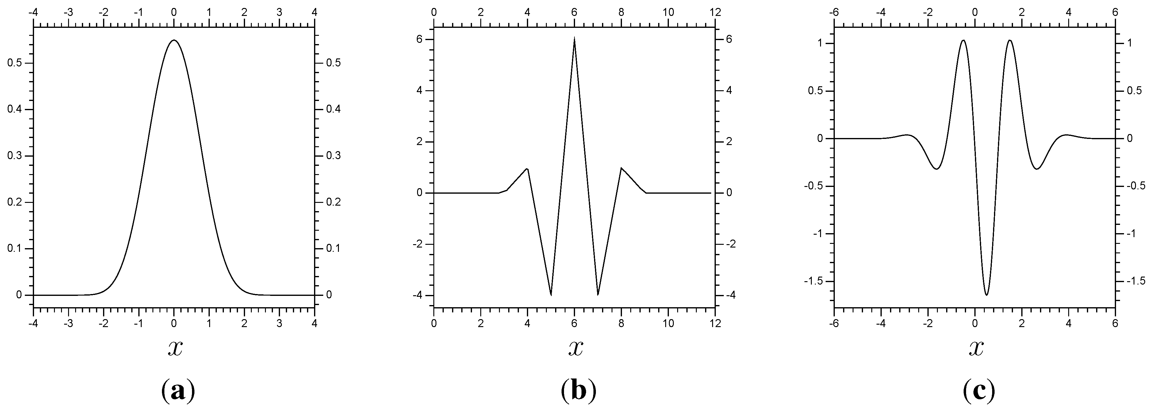
6]). The first example uses a scaling function
φ equivalent to the fourth order spline function, which is shown in
Figure 1, along with its second derivative
and its dual
. The figure also shows the corresponding wavelet
ψ, along with its second derivative
and its dual
.
Figure 1.
Top: The wavelet pair corresponding to the spline function , its second derivative and dual re-centered at . Bottom: The same for the corresponding wavelet. (a) ; (b) ; (c) ; (d) ; (e) ; (f) .
Figure 1.
Top: The wavelet pair corresponding to the spline function , its second derivative and dual re-centered at . Bottom: The same for the corresponding wavelet. (a) ; (b) ; (c) ; (d) ; (e) ; (f) .
A wavelet decomposition uses variants of the form
Notice that
and
for all
(using the
norm). Also, notice that the functions become more localized (
i.e., have their support reduced) as
j becomes more negative, while
k determines the location of
or
. Notice also that
and
are equal except for a translation of one, and that
and
are equal except for a translation of
. As a result, more negative values of
j do not just make the functions
and
more localized, but also reduce the space between them. One key property of the scaling function,
φ, and wavelet,
ψ, is that they can be written in terms of the finer scaling functions
, so
for constants
and
.
These functions create subspaces of
of the form
This definition and (
2.2) mean that
and, more generally,
for all
. We also get
, which in turn makes
As a result, any function
(
) can be expressed using different, but equivalent, sets of basis functions from the spaces
and
. First, by the definition of
,
However, assuming that
, we can write it in terms of
, so
Continuing this pattern, we can get
which can be expanded to
and further. Basically, there is a starting function of the form
which is simply an approximation of
f in the coarse resolution space
. Then functions
are added to correct that approximation. So, any function
has a unique component in
(equal to the projection of
f onto
when orthogonal wavelets are used), an approximation containing only the coarser, large-scale, features of
f. The finer, smaller scale, features of
f are found in the spaces
to
.
3. Multi-Scale Method
We propose a new wavelet method for solving time-dependent partial differential equations, specifically multi-scale problems that require implicit time-discretization. The method exploits the form of the wavelet decomposition to divide the implicit system created by the time-discretization into multiple, smaller, systems that can be solved sequentially. One can, if certain requirements are taken into account, compute implicit time steps at multiple spatial resolutions. Most importantly, these resolutions are solved sequentially, and kept consistent so they need only be solved once per time step. For non-linear problems, where even a linearized scheme (such as that in Equation (
7.2)) requires solving a new system every time step, this can greatly reduce computational expense. The key idea is to divide the system to be solved into two, smaller, systems that can be solved separately. First, we have a coarse resolution
over the whole domain Ω, called the large-scale system. The next system has the finer resolution
only covering the subset
, called the small-scale system (with
). This arrangement allows the two systems to be solved sequentially. First, the large-scale system is solved, in
over Ω, and the resulting coefficients that are within (or near) Λ are converted so that they can be expressed in terms of the small-scale. Those coefficients are included in the calculations for the new small-scale system. Next, the large-scale (
) components of the newly calculated small-scale system are converted to the form used in the large-scale, and added to the earlier large-scale values. This finishes the time step. Note that the two systems, large and small-scale, are solved separately.
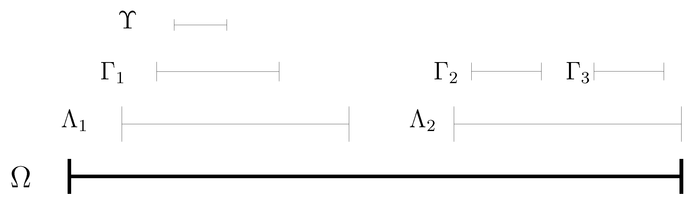
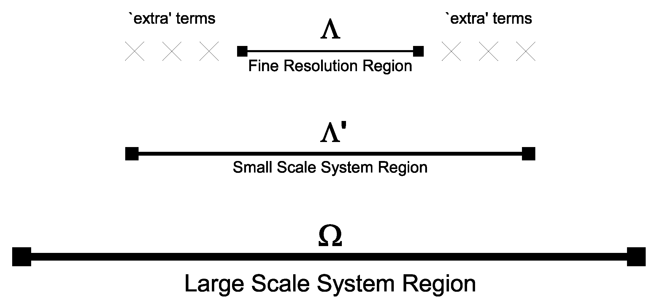
Depending on how the discretization is implemented, the two systems can be the same size (that is, have the same number of coefficients). In fact, this arrangement can be done with any number of systems, possibly nested, as shown in
Figure 2. As long as their domains are either nested or disjoint, any number of systems can be used. That the different systems can be solved separately is the advantage here. A pair of systems sized
will be quicker to solve than a single system sized
.
Figure 2.
A diagram of several nested small-scale systems of a domain Ω.
Figure 2.
A diagram of several nested small-scale systems of a domain Ω.
4. Implementation
In this section we describe the basic implementation of the method: The dividing of an implicit time step into two, separately calculated, systems. This concept should be compatible with many features of multi-scale methods, (i.e., making the large- and small-scale systems use adaptive decompositions). However, we will not include any, to avoid additional complications. The numerical experiments will be kept as simple as possible, as well.
To explain our method in detail requires a certain level of notation. We shall look at a one-dimensional example, though the general concept behind the method can be expanded to any number of dimensions. For instance, our second numerical example uses a decomposition of a two-dimensional domain Ω via tensor product between a Fourier decomposition in the x direction and a wavelet decomposition in the y direction. This allows the small-scale domain Λ to be of the form , i.e., to cover the entire x domain and a subset of the y domain. If the decomposition was via a tensor product with wavelet decompositions in both directions, then we could use a subdomain Λ that is smaller, with finer resolution, in either direction, or both.
The actual functions we shall be dealing with are those of the form
Recall that wavelet decompositions are in the spaces
and
,
, as defined in (
2.3) and (
2.4). In
Section 2 we discussed how there are multiple ways of expressing a function via wavelet decomposition. Since the specific form of the decomposition is relevant to any wavelet-related method, a means of expressing these differences becomes helpful.
All functions in the space
and
can be characterized in terms of the coefficients of their wavelets and scaling functions. The wavelet (
ψ) coefficients are written
, the scaling function (
φ) coefficients are written
, with
j relating to resolution and
k relating to location. The coefficients
are best organized into vectors of the form
The same can be done with the sets of coefficients
, creating vectors
of the form
Any decomposition of the form in (
4.1) has an equivalent vector
Any function
can also be decomposed directly into
via
with a vector
, which has the same number of components as the vector in (
4.4). The setup discussed in
Section 3 focused on two different levels of resolution,
and
, with
. One helpful way of writing this is to define a vector
, containing all the necessary coefficients for
, and a vector
containing all the necessary coefficients for the spaces
to
. This setup, using
and
, would result in vectors of the form
The result of this setup is that any function in
can be expressed in terms of a vector of the form
, and any function in
can be expressed in terms of a vector
.
Next, we have two different domains to use: Ω and . The vector has all the coefficients from the space over the entire domain Ω. Now we must consider vectors relating only to . Whether a coefficient can be considered relating to Λ depends on its scaling function . We use biorthogonal scaling functions and wavelets that are symmetric, with finite support. As a result, we designate or to be within Λ if the center of the function’s support is strictly within Λ. Other options would probably work, such as defining or to be in Λ if their supports intersect Λ. A subscript Λ, for , restricts the coefficients in to those relating to the smaller domain Λ. This will be standard practice throughout this paper. If a subscript Λ is added to a vector or matrix, that means that the vector or matrix is restricted to the smaller domain Λ, with coefficients relating only to Λ.
Now we take a linear partial differential equation of the form
where
L is a linear differential operator
As
L is linear, we discretize it using a matrix
M. The idea is for
M to calculate the effect of
L restricted to
. So, if the function
is expressed in terms of
, then
This matrix
M can be calculated via a Galerkin or collocation method, so long as it is accurate in approximating
L. Our earliest tests of this method used a Galerkin method. In this paper, the examples will be calculated via a collocation method, discussed later in
Subsection 7.2. Boundary conditions are a potential issue. To keep the equations in this section clean, we will be ignoring the boundary conditions, or assuming that they are satisfied via the wavelet decomposition and
M. Our later examples use the method effectively on a problem with zero boundary conditions and on a problem with constant, non-zero, boundary conditions. Our approach for satisfying zero boundary conditions is discussed in
Subsection 7.2.
The method is meant for use with an implicit time-discretization. Here, and in the rest of the paper, we shall illustrate the implementation of the method using the second order Adams-Moulton scheme for the time-discretization. This particular scheme is ideal since it is simple and, most importantly, implicit. Combining that time-discretization with the matrix
M gives us the time step
We also use the block decomposition
Assume that the vectors
and
have
and
components, respectively. The matrix
A will have
rows and columns and
D will have
rows and columns. The matrix
B will have
rows and
columns, and
C will have
rows and
columns. Note that while
A and
D are square, they do not have to be equal in size. In fact, our main example will usually give
A four times as many rows and columns as
D.
Now we separate the time step in Equation (
4.9) into two systems. First, we have the large-scale system, with functions in the space
over Ω, characterized by vectors of the form
. We also have the small-scale system with functions in
over Λ, characterized by vectors of the form
. Recall that
has only the components of
corresponding to the functions
in Λ. The large-scale system is at the limited resolution
, and so uses the matrix
D to model the operator
L from (
4.7). The small-scale system is expressed in terms of a matrix
of the form
where
,
,
and
are composed of the elements from
A,
B,
C and
D that are related to Λ.
Example 4.1 Using the domains and and the space , we shall take a look at getting from D.
In this example, the vector
has 79 components: The functions
are at points separated by a distance of
, and so are at points
,
,
… ,
. The matrix
D, which is a discretization for the differential operator
L restricted to
, is a square matrix. Multiplication (on the left) by this matrix takes the
coefficients from a function
in the vector
, creating the vector
, the
approximation of
. We can write it as
The matrix
only operates on the coefficients of functions
restricted to Λ. As a result, the number of rows and columns of
have to be equal to the number of
coefficients in Λ. As a result, it is smaller:
The first step is to use a time-discretization to find a temporary approximation of
, which we shall call
. Using the second-order Adams-Moulton method yields the large-scale system
This calculates the time step on Ω at the large-scale resolution
. What we want next is to calculate the time step on Λ at the small-scale resolution
. However,
and the newly calculated
have to be included. So, we use the components of
and
that are in Λ, which we call
and
, respectively. These are used in the system
Note the presence of
, a corrector term for the temporary approximation
. The final step is to take
, rewrite it in Ω as
, and add it to
for
This setup is consistent with the time-discretization. Since
, the restriction of
to Λ will be
Next, we will rewrite that expression using
The last term in (
4.16) is going to be smaller than the others, considering the restriction to
followed by a restriction to Λ. In the context of the small-scale system, the last term in (
4.16) can be viewed as representing influences that are similar to boundary conditions: Influences consistent with the problem that come from outside the region being calculated (Λ, in this case). This term, being somewhat cumbersome to write and read, will not be written in the next expressions. We will simply replace the first term in (
4.16) with the second (they are, at least, approximately equal). This substitution yields
which matches the second order Adams-Moulton discretization.
6. A Test Problem
To illustrate the application of the method, and confirm that it can work, we test it on a one dimensional problem involving Burgers’ equation. Burgers’ equation is appropriate because it is not linear, its expression is fairly simple, and because it can be easily set up to require fine resolution in a small region and so benefit from the method we are testing. Note that we are deliberately keeping things very simple. We will use fixed Λ subdomains, and fixed resolutions. The method looks to be compatible with many types of adaptive schemes, and other expansions. However, in this paper, we want to ensure that the method can deliver consistent results, with no additional complications. We therefore use the simplest version of the method, without these additional features.
We solve for the function
,
,
, satisfying
with boundary and initial conditions
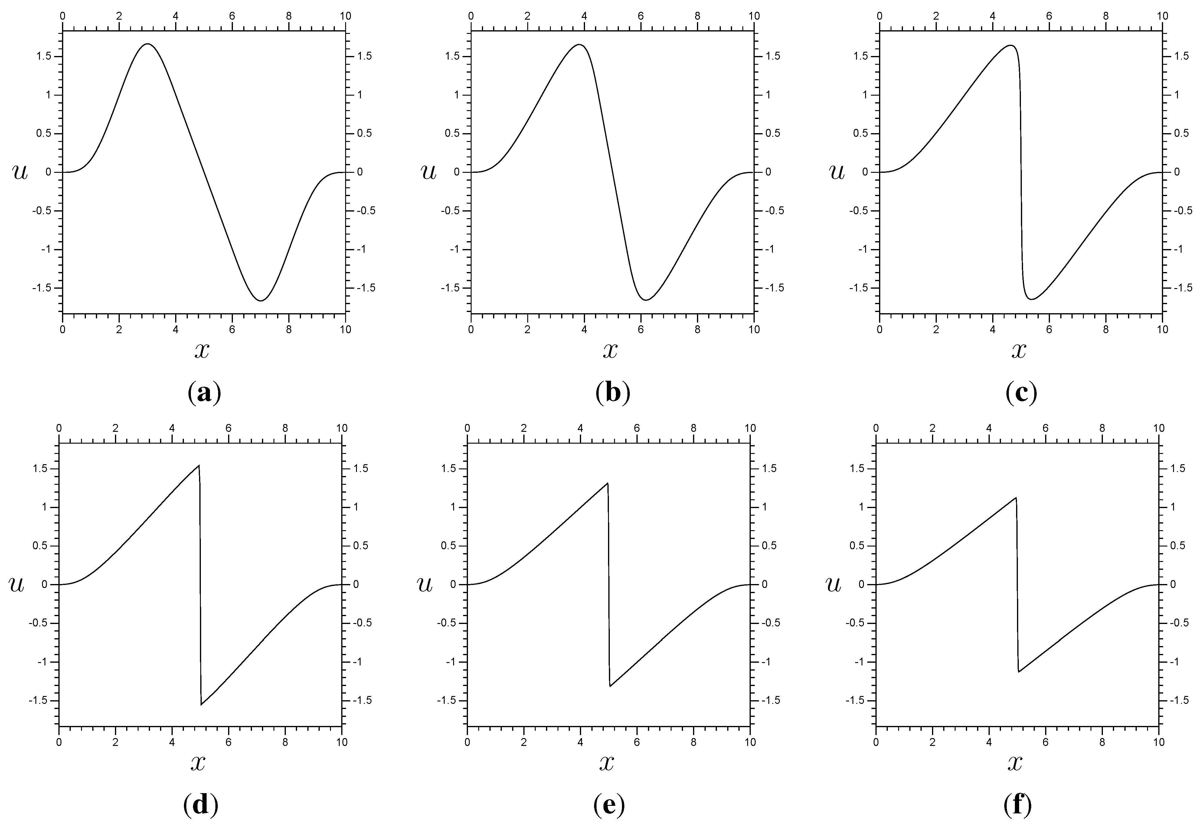
The function
is plotted in
Figure 3 (a). The exact value of
is
using
φ from
Figure 1. This choice of initial condition will require some explanation. First, we use an initial condition in
to simplify the required programs and to avoid any error at
. This means that all different models/resolutions start at zero error. The general shape chosen relates to the behavior of Burgers’ equation, mainly the effect of the
term. If we set the viscous parameter,
ν, to zero then the solution becomes
meaning that the characteristics will start at points
and have slopes equal to
. Of course, if
then this effect will be changed, but the basic nature, and directions, will be much the same. Now consider what this means for
in
Figure 3. As shown in this figure, the two peaks will approach each other as the time increases, colliding at
. What happens when they meet depends on the magnitude of
ν. If
, then the characteristics will intersect, resulting in a singular solution. If
then the peaks will collide, but not cause an infinite slope. Instead, the translation will cease, and the solution will converge to zero under the influence of the viscosity (see
Figure 3). So, instead of an infinite slope at
, the solution will have a finite slope dependent on the magnitude of
ν. Increase
ν and the resulting slope at
will get smaller. Decrease
ν and the slope at
will be greater. A very steep slope at
will make proper expression of the solution very difficult for a coarse resolution
space. The results shown here, with
, require at least
for reasonable results (using our wavelet/scaling function pair).
Figure 3.
Results for Burgers’ equation with resolution and time step . (a) ; (b) ; (c) ; (d) ; (e) ; (f) .
Figure 3.
Results for Burgers’ equation with resolution and time step . (a) ; (b) ; (c) ; (d) ; (e) ; (f) .
9. Results
The most accurate (and stable) results use linear components derived from a full operator decomposition matrix
M (see
Section 4). Doing so results in the term
from (
8.9) being equal to a zero matrix, so there is no need for a matrix
J (see
Subsection 8.1) for the linear components of
L. A matrix
(again, see
Subsection 8.1), is required for the non-linear derivative terms. Our first set of multi-scale results use
on
and
on
. They also use three “extra” terms and
meaning that the non-linear effect on the “extra” terms in
is removed entirely. The results are in
Figure 6, and the error (difference between the multi-scale, from
Figure 6, and control results, from
Figure 3) is in
Figure 7. They show little difference from the full resolution
results. Remember that these results use half as many terms, in total, and the method solves them in approximately half sized sections. As a result, the average time step for the
system takes about 0.988 seconds (on a 2.5 GHz processor, standard for the remainder of the paper), while the average time step for the
/
multi-scale system takes about 0.0337 s. So, the multi-scale system gives results differing by 0.001, and takes about 3.4% as much time to compute.
Next, we need to confirm that the method can converge towards the results of the fine resolution system. To do so, we use a full domain
and compare it to a scheme using
with localized
. An increase in the size of Λ and the number of “extra” terms should cause the resulting error to decrease. The multiplier
is set to have a zero for each “extra” term, then one more zero followed by
, 1, and so on. The problem is the same, with
, as is the size of the time step,
. One interesting result is that the error in the interior of Λ becomes so small that it becomes insignificant next to the errors near
and
. See
Figure 8, and notice that the error on the boundary stays constant as Λ increases in size. The error near
and
is due to lack of resolution around the boundary. No matter how large we make Λ, or how close Λ gets to the boundary of Ω, that error stays constant (to within machine precision). We are mostly interested in the accuracy near the center of the domain, the modeling of the collision between the peaks. Also, the translation from the boundary to the center is trivial, meaning that the accuracy near the boundary has a minimal effect on the interior. So, we shall simply ignore
and
when calculating the error. In
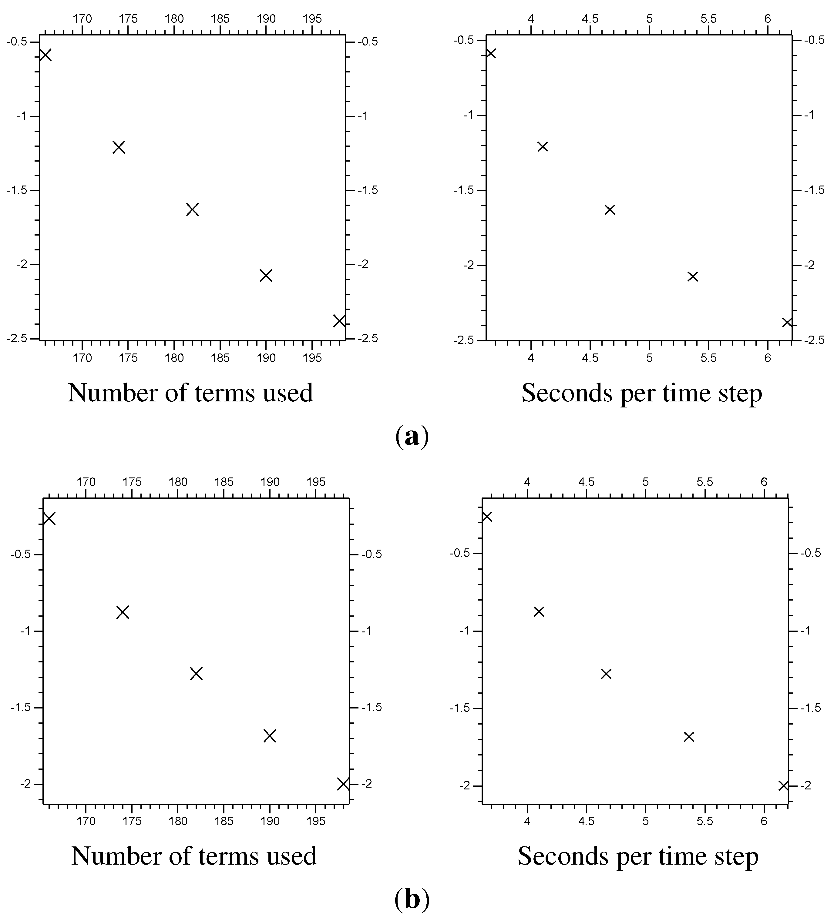
Figure 9 we have a set of plots of the errors (numerically approximated using a resolution of
elements per unit) of the different multi-scale systems, compared with the full domain
system. These are calculated at
, only on
.
Table 1 summarizes the
Figure 9 results (notice that the “Terms” column relates to the horizontal axis for the plots on the left in
Figure 9, and the “Time” column relates to those on the right). To put these results in perspective, the difference calculated in
Subsection 7.3 between the
control results and a much more accurate
model has
,
and
differences of
,
and
, respectively, on the subdomain
. Basically, we have found solid evidence that the error resulting from our multi-scale method is trivial next to the error stemming from using a limited resolution of
.
Figure 6.
Results for Burgers’ equation using the components from
Section 8. These use
with localized
and three “extra” coefficients
around
. It also uses
values of 0, 0, 0, 0,
, 1, 1,
etc. The time step size is
. (
a)
; (
b)
; (
c)
; (
d)
; (
e)
; (
f)
.
Figure 6.
Results for Burgers’ equation using the components from
Section 8. These use
with localized
and three “extra” coefficients
around
. It also uses
values of 0, 0, 0, 0,
, 1, 1,
etc. The time step size is
. (
a)
; (
b)
; (
c)
; (
d)
; (
e)
; (
f)
.
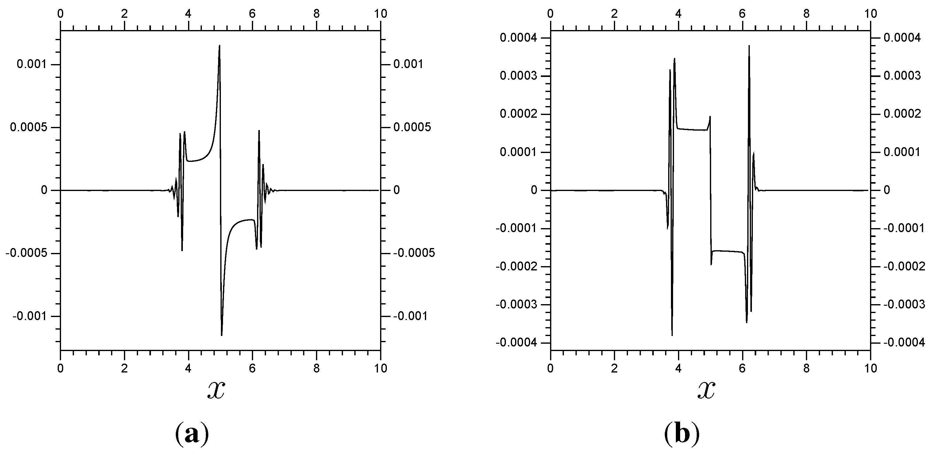
Figure 7.
Results of a multi-scale system for Burgers’ equation compared with a full resolution system. The error shown is the difference between the
/
results from
Figure 6 and the full
resolution results from
Figure 3. (
a) Error at
; (
b) Error at
.
Figure 7.
Results of a multi-scale system for Burgers’ equation compared with a full resolution system. The error shown is the difference between the
/
results from
Figure 6 and the full
resolution results from
Figure 3. (
a) Error at
; (
b) Error at
.
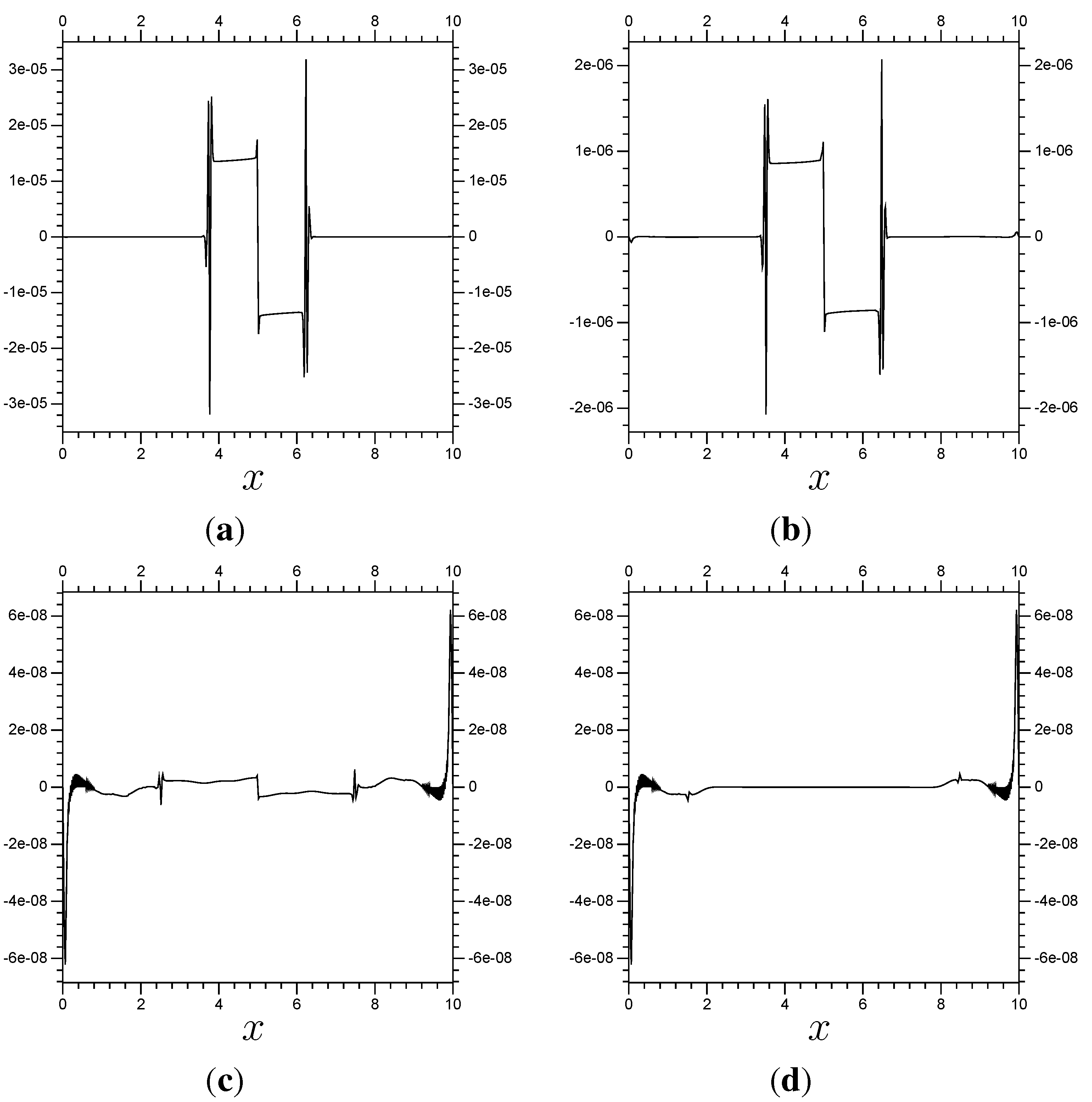
Figure 8.
Error from results using with localized . The error is the difference between the multi-scale results and the control results, all calculated at . The multi-scale results differ in their Λ sub-domains. All use 4 “extra” terms per boundary of Λ. (a) ; (b) ; (c) ; (d) .
Figure 8.
Error from results using with localized . The error is the difference between the multi-scale results and the control results, all calculated at . The multi-scale results differ in their Λ sub-domains. All use 4 “extra” terms per boundary of Λ. (a) ; (b) ; (c) ; (d) .
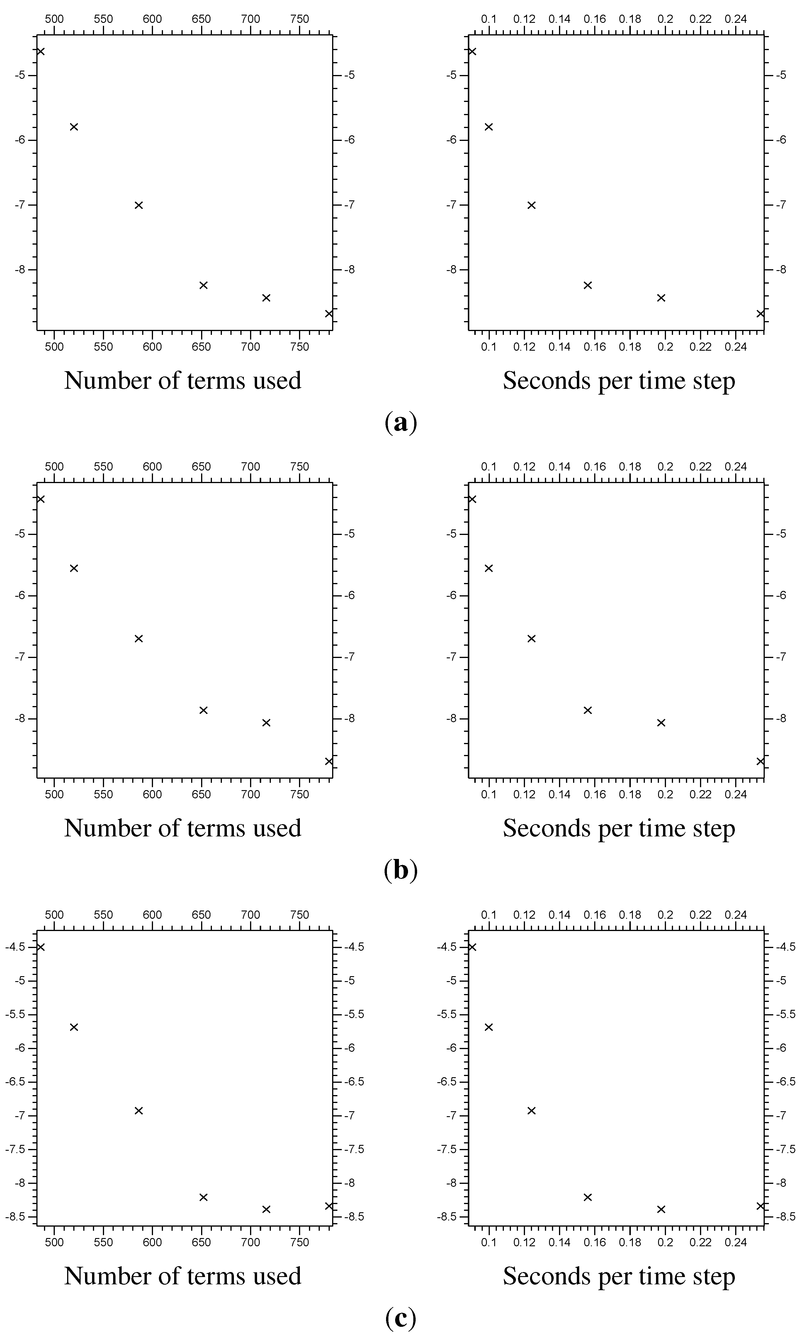
Figure 9.
Error from multi-scale systems, compared with system size and computational time. The system size is the total number of coefficients
and
used in the systems (also seen in
Table 1). The computational time is the average time taken to calculate a single time step, in seconds (all using the same computer). The vertical axis is the
of the error, the difference between the multi-scale results and the fine resolution control results on (1.5, 8.5). (
a)
of the
error; (
b)
of the
error; (
c)
of the
error.
Table 1.
Burgers’ equation error for multi-scale systems. By “Time” we mean the average computing time (in seconds) per time step. Note that the errors are only calculated in the region .
Table 1.
Burgers’ equation error for multi-scale systems. By “Time” we mean the average computing time (in seconds) per time step. Note that the errors are only calculated in the region .
| Λ | “extra” | Terms | Time | Error | Error | Error |
|---|
| 4 | 128 | 0.0904 | | | |
| 5 | 138 | 0.0998 | | | |
| 6 | 156 | 0.1241 | | | |
| 7 | 174 | 0.1560 | | | |
| 7 | 190 | 0.1977 | | | |
| 7 | 206 | 0.2541 | | | |
| control results | 0.9888 | |
10. A Further Test
Now we extend the method to a non-trivial problem, one that requires fine resolution in one of its two spatial dimensions. We shall use the same time stepping scheme, the same multi-scale method, and the same modifications (the “extra” terms and matrix
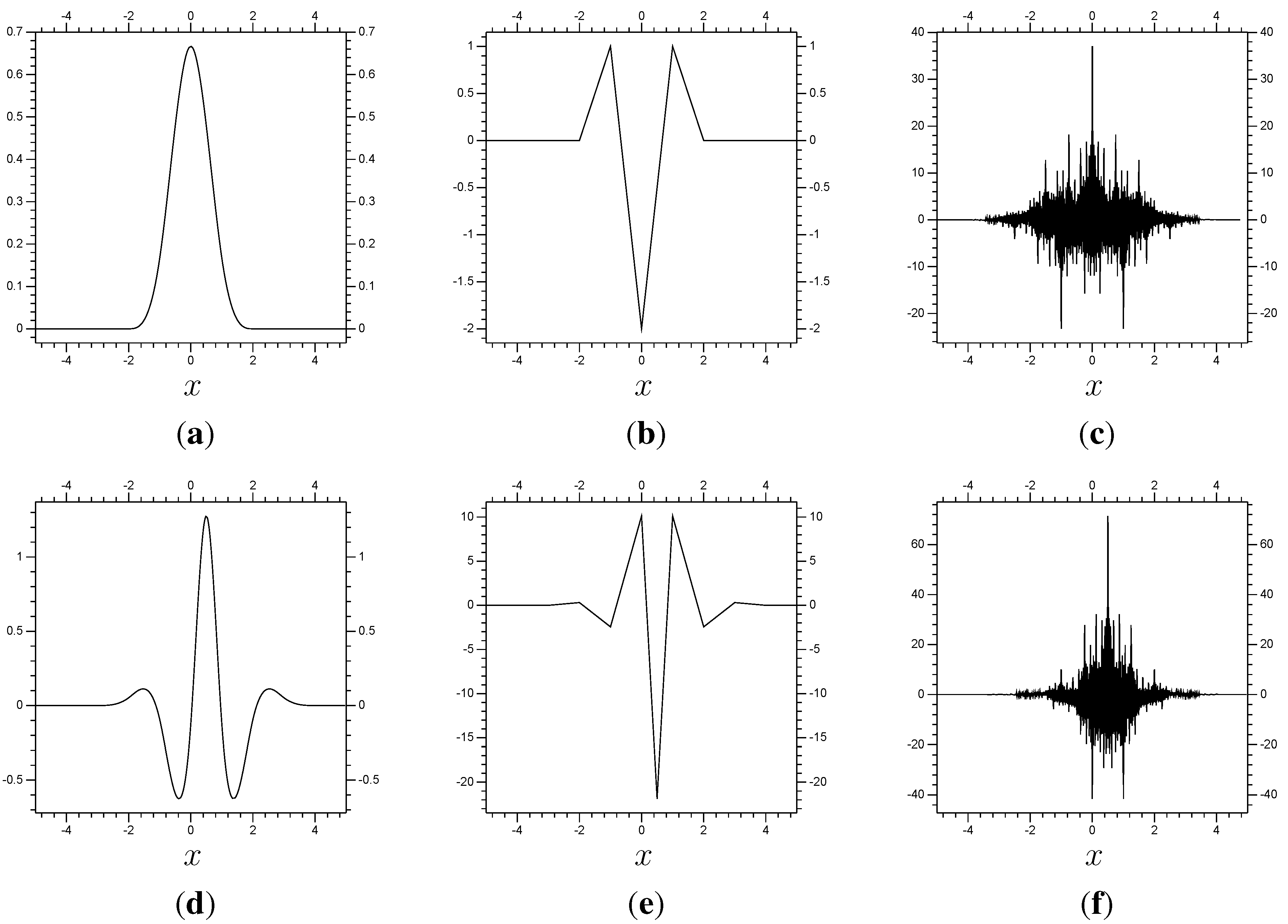
J). However, the differential equation has a fourth spatial derivative, and so is best approached with a higher order scaling function and wavelet pair, seen in
Figure 10.
Figure 10.
The spline function , our scaling function. Next, and our wavelet, ψ. (a) ; (b) ; (c) .
Figure 10.
The spline function , our scaling function. Next, and our wavelet, ψ. (a) ; (b) ; (c) .
10.1. The Rossby Wave Problem
The problem is time-dependent on an
x,
y, domain, with reference lengths
and
, respectively. There are periodic boundary conditions in the
x-direction, and time-independent Dirichlet boundary conditions in the
y-direction. First, we shall nondimensionalize the problem, converting the domain to
and
. The primary effect of this is that the Laplacian operator
will be re-scaled to
For further details on the problem, see [
19].
The problem is based on the nondimensionalized barotropic vorticity equation
(see ([
20] [p. 637]) for details) with the (real) function
the stream function on the domain (not a wavelet). The velocity component in the
x-direction is equal to
and the
y component is equal to
. The variable
x represents longitude (east-west) and
y the latitude (north-south). The coefficient
β relates to planetary rotation and
ν is the viscosity coefficient.
Next we decompose the stream function Ψ into two components,
with
ϵ small relative to Ψ and
. The function
is the stream function of the basic flow. We are assuming that the basic flow is a shear flow, with velocity only in the
x-direction, meaning that
is a function of
y only. We set
, a known function. The Rossby waves are given by
, the stream function representing small perturbations of the basic flow, with the matching vorticity perturbation
.
Substituting (
10.3) into (
10.2), we obtain
which becomes
(with
being the third derivative of
). We shall ignore the last
y dependent term, since
is small, and even when
we shall keep
ν much smaller than
ϵ, so (
10.5) becomes
Our examples will use
, meaning the basic flow will be very nearly constant in the regions near
and
, (at
and
, respectively). Second, the basic flow velocity will be zero at
. As we shall see, these properties of
have interesting implications for
P.
The boundary conditions are for and (recall that the boundary conditions are periodic in x). We shall have those boundary conditions phased in gradually (over or so) to smooth out the discontinuity, starting at zero and smoothly increasing to . Notice that the boundary conditions are all composed of , so they can be written in terms of . If we use the linear form of the problem (set ), then P (and Z) can be written using only functions in the x-direction (each multiplied by a function of y and t). The initial condition is simply .
Now we go to the simplest case, set
along with
ϵ. If we assume that the problem has a steady state, we can find that it will have the form
In the area immediately around
,
is approximately one and
is approximately zero. The problem becomes
with a solution of the form
,
. As a result, recalling that the boundary condition at
is
, the steady state is
approximately, near
. The more general observation is that the problem in (
10.7) has a singularity when
, so at
. The singularity at
means we require fine resolution at that location in order to accurately model the problem. The effect of the critical layer, the region around
, on the problem is well known. The function
P, which has the form of (
10.9) near
, will propagate downwards, curve slightly, then stop around
(see
Figure 11B). This behavior is consistent with that found in the literature:
Figure 11B is consistent with all the
P (equivalent) plots in [
19], and virtually identical to ([
19] [
Figure 2a]). The behavior of the perturbation velocity
is also fairly well known.
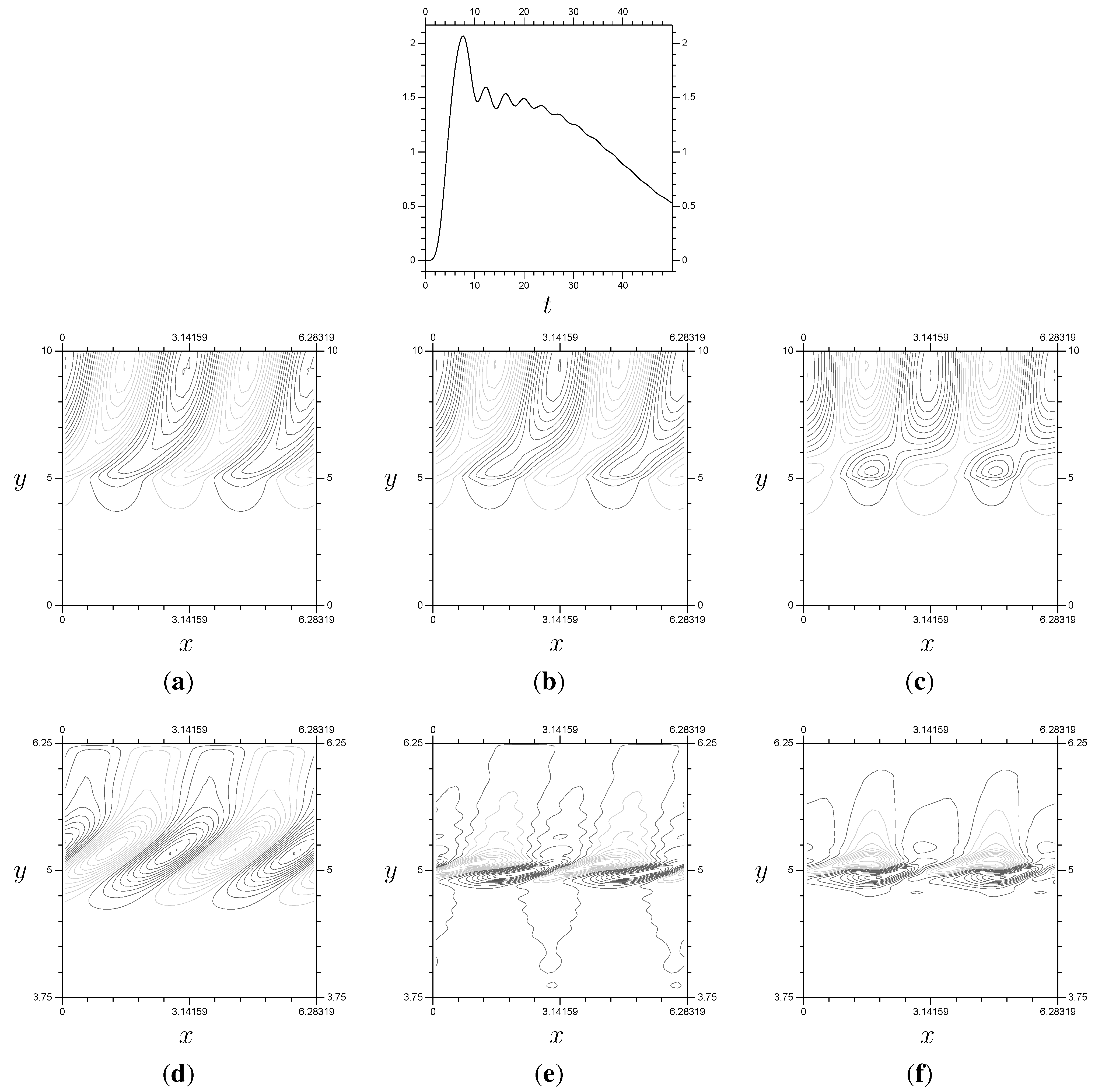
Figure 11 contains plots of
Z at different times. The general
Z shape expected for the linear problem is the waves around
, seen in
Figure 11. Notice that the amplitude of
Z near
is much higher than that anywhere else, and that the waves in the center get more tightly concentrated as
t increases. As we shall see, this results in a greater requirement for fine resolution in the center as
t increases, which is what we would expect considering the singularity at
. The shape of our
Z plots in
Figure 11 matches well with ([
19] [
Figure 18a]) and ([
21] [
Figure 4]), even though our results use different domains and boundary conditions.
Apart from
P and
Z, there is one more quantity we shall use to check the accuracy of our results. We shall be interested in the momentum of the system, specifically the averaged
x directional momentum flux of the region
. Information on momentum as it relates to fluid dynamics can be found in any text on the subject, such as ([
20] [p. 88]). For our purposes, it suffices to say we calculate the momentum going in and out of the region via the integral
at
and
. The change in the
x-averaged momentum flux across the region
is equal to
although the first integral is approximately zero since
for
. In this particular system, there are some very clear expectations. First, the linear problem is expected to result in a positive flux at the beginning, so momentum flowing into the critical layer. In ([
22] [
Figure 5, line 1]) and ([
19] [
Figure 3]), the flux for the linear problem can be seen reaching its maximum early, then lowering and stabilizing at a positive value. This is the expected behavior of the linear problem, see
Figure 11a. When the non-linear interactions are included, the critical layer is expected to reflect some of the momentum. The flux, as seen in ([
22] [
Figure 5, lines 2,3]) and ([
19] [
Figure 3b]), is expected to reach its maximum value early, then reduce down to zero and begin oscillating around zero. Later, we shall test our numerically derived results against these expectations.
Figure 11.
(Top) The flux (a), steady state for P (b). (Bottom) the progression of Z at in the x-y plane, from left to right. These use , and . Notice that Z increases in amplitude and decreases in wavelength as time increases. (a) The Flux; (b) P; (c) Z, ; (d) Z, ; (e) Z, .
Figure 11.
(Top) The flux (a), steady state for P (b). (Bottom) the progression of Z at in the x-y plane, from left to right. These use , and . Notice that Z increases in amplitude and decreases in wavelength as time increases. (a) The Flux; (b) P; (c) Z, ; (d) Z, ; (e) Z, .
10.2. Linear Results
The key observation for the linear version of the problem (when
) is the steady state expected by the theory, briefly discussed in
Subsection 10.1. As
t increases, the linear solution eventually converges to the steady state given in
Figure 11b (as long as we are using our usual
). However, as shown in
Figure 11, this results in
Z requiring very fine resolution around
. As a result, what we actually see in numerical computation is the perturbation stream function
P reaching the steady state (or close to it), holding, then, after some time, becoming completely inaccurate. Generally, without viscosity, our computed values of
P are accurate up to approximately
using resolution
, as shown in
Figure 12 and
Figure 13.
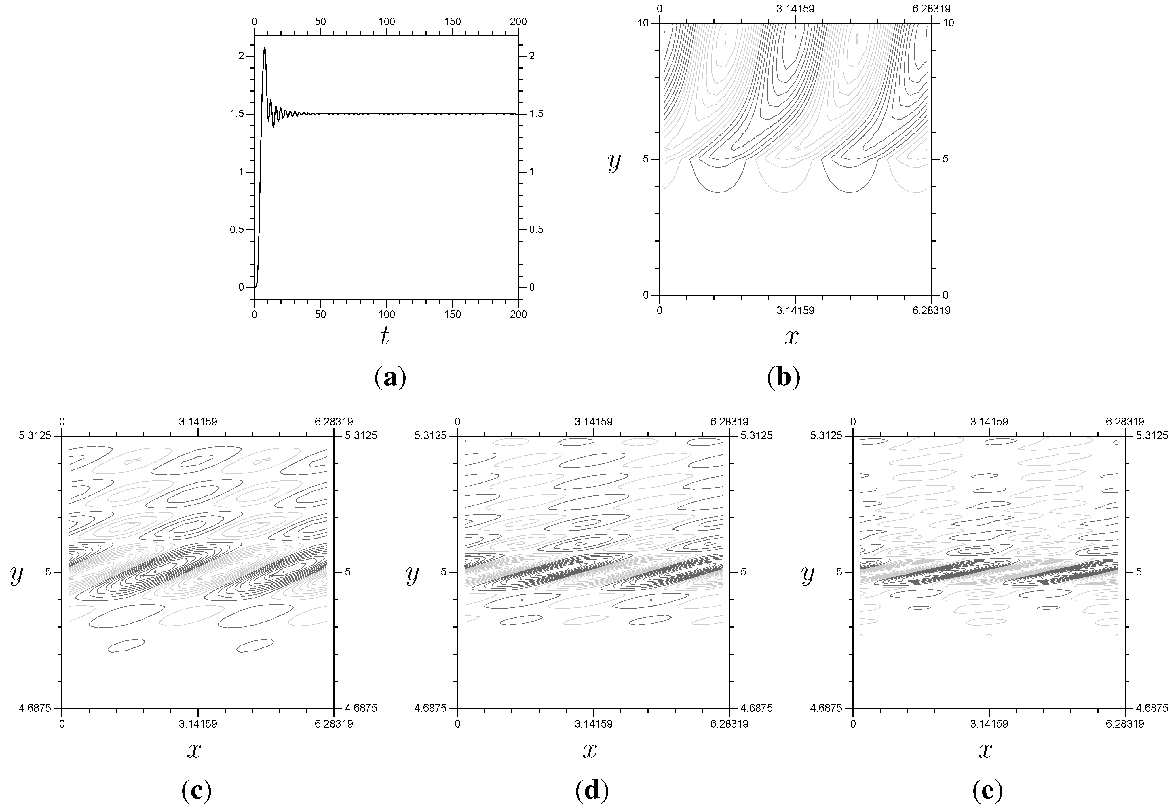
Figure 12.
The results from a linear system. Notice that (the x averaged momentum flux) remains stable until . These results use a “switch-on” function for the boundary condition values equal to , , , and no viscosity. (a) ; (b) P, ; (c) Z, .
Figure 12.
The results from a linear system. Notice that (the x averaged momentum flux) remains stable until . These results use a “switch-on” function for the boundary condition values equal to , , , and no viscosity. (a) ; (b) P, ; (c) Z, .
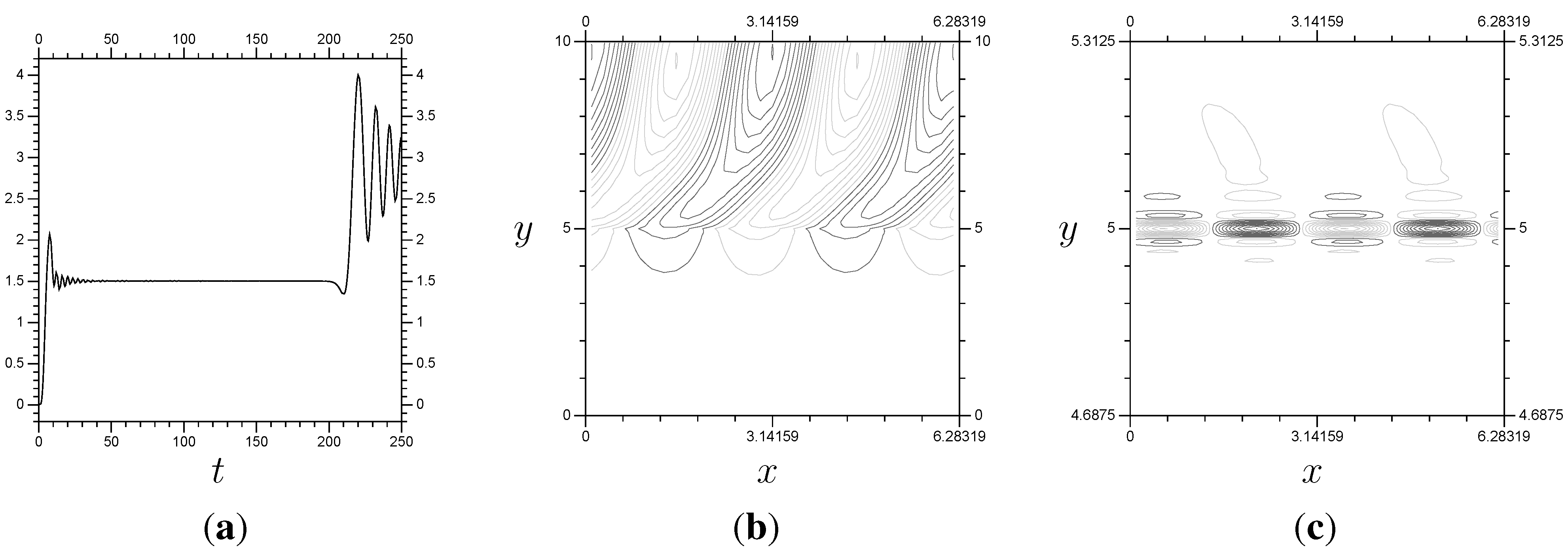
Figure 13.
The results from a linear
system. Notice that
remains stable until
, where
Z is following the same pattern seen in
Figure 12c. These results are based around the same problem as those in
Figure 12, just with a different resolution. (
a)
; (
b)
P,
; (
c)
Z,
.
Figure 13.
The results from a linear
system. Notice that
remains stable until
, where
Z is following the same pattern seen in
Figure 12c. These results are based around the same problem as those in
Figure 12, just with a different resolution. (
a)
; (
b)
P,
; (
c)
Z,
.
As seen in the
Z plots, the key information is around
, so that is the location for the small-scale system. The real test is whether the multi-scale results will be accurate (stable,
etc.) over the same time frame. The
single system results are accurate to approximately
(
Figure 12). In
Figure 14, we have results using
everywhere and
on
, showing an accurate solution of the problem up to
, so the multi-scale method works for the linear problem. Note that the multi-scale arrangement has
terms per Fourier mode, and the two systems are solved separately. The full
system has 639 elements per Fourier mode, and the system has to be solved all at once.
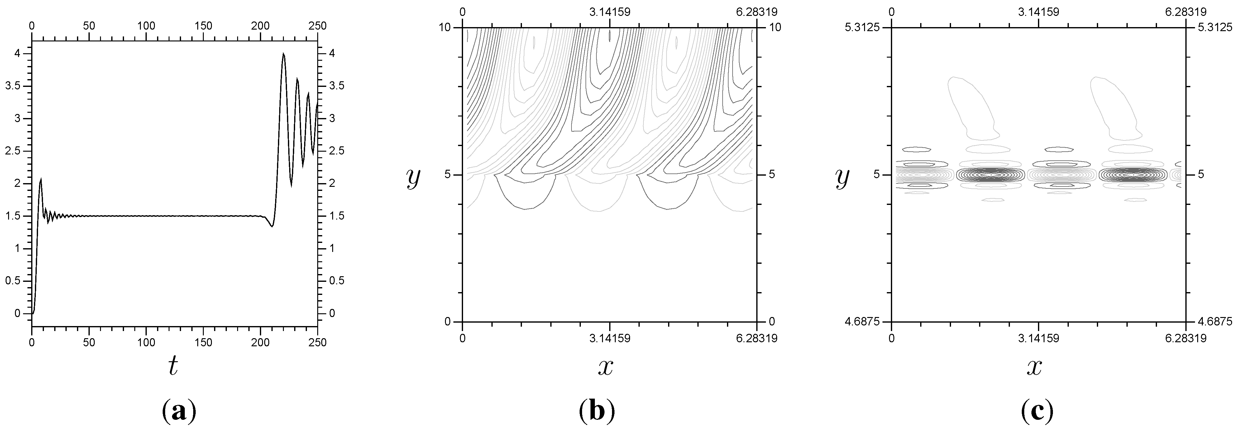
Figure 14.
Results from a
with localized
double system. The small-scale is over
, and 3 “extra” terms are used over both interfaces of Λ. There is a little instability in the flux around
, but this arrangement is very close to the full
control system, found in
Figure 12. (
a)
; (
b)
P,
; (
c)
Z,
.
Figure 14.
Results from a
with localized
double system. The small-scale is over
, and 3 “extra” terms are used over both interfaces of Λ. There is a little instability in the flux around
, but this arrangement is very close to the full
control system, found in
Figure 12. (
a)
; (
b)
P,
; (
c)
Z,
.
10.3. Non-Linear Results
The actual benefits of the multi-scale system exist primarily for non-linear problems, so we shall switch to the non-linear version, with
. The linearization scheme used on Burgers’ equation (see (
7.2)) will be used again.
There is one more, significant, issue: We shall need many more Fourier coefficients to properly express the x direction when . With the boundary conditions just multiples of , and with initial conditions of zero, the linear problem’s solution can be written in terms of in the x direction. If we have with the same boundary and initial conditions, then the problem will require , , in the x direction. We use , so the even Fourier modes will be relevant. Obviously, we have to restrict the number of Fourier modes we calculate to a finite number, and use a pseudo Fourier scheme to approximate and . The functions P and Z are real, so modeling the Fourier modes (for ) requires K complex values and one real value to keep track of, which are effectively real values.
So, we have to create and solve a new linear system at every step, and the systems themselves will be significantly larger. As a result, we shall keep the y resolution down to a manageable , or 16 elements per interval of length one, so 159 total on . Combined with 11 elements for the x direction and that makes 1749 real coefficients in total. The boundary conditions are the same, and , as before. We shall include some viscosity, , to stabilize the system and make the resolution plausible. We use , and the size of the time step is .
Our multi-scale results use the method that was applied to Burgers’ equation in
Section 8. We use three “extra” terms and a
J multiplier with
The linear components of the calculation are derived the same way as in
Section 8 as well, from a system using the finest resolution over all Ω.
As discussed at the end of
Subsection 10.1, the flux for the non-linear problem is expected to reach its maximum early, then reduce down to zero and begin oscillating around zero. As for
P, it is expected to develop waves similar to the linear problem, at least initially. As
t increases, we can expect the tip of the waves in
P, the parts near
, to break from the rest and create separate, somewhat circular, shapes. This behavior is shown nicely in ([
19] [
Figure 2b and
Figure 14b]). Other than the expectation of greater complexity, we shall say little of
Z. We shall, however, use
Z to check the accuracy of the multi-scale results.
When
, the flux is expected to quickly reach the steady state of the linear system, then slowly reduce to zero and begin oscillating around zero. Take a look at
Figure 15a–f. The value
is not high enough for the flux to reach zero during
, so instead we see a reduction towards zero for the
model. We set
as our top resolution, the results we want to duplicate efficiently with the multi-scale method. Our large-scale resolution is
.
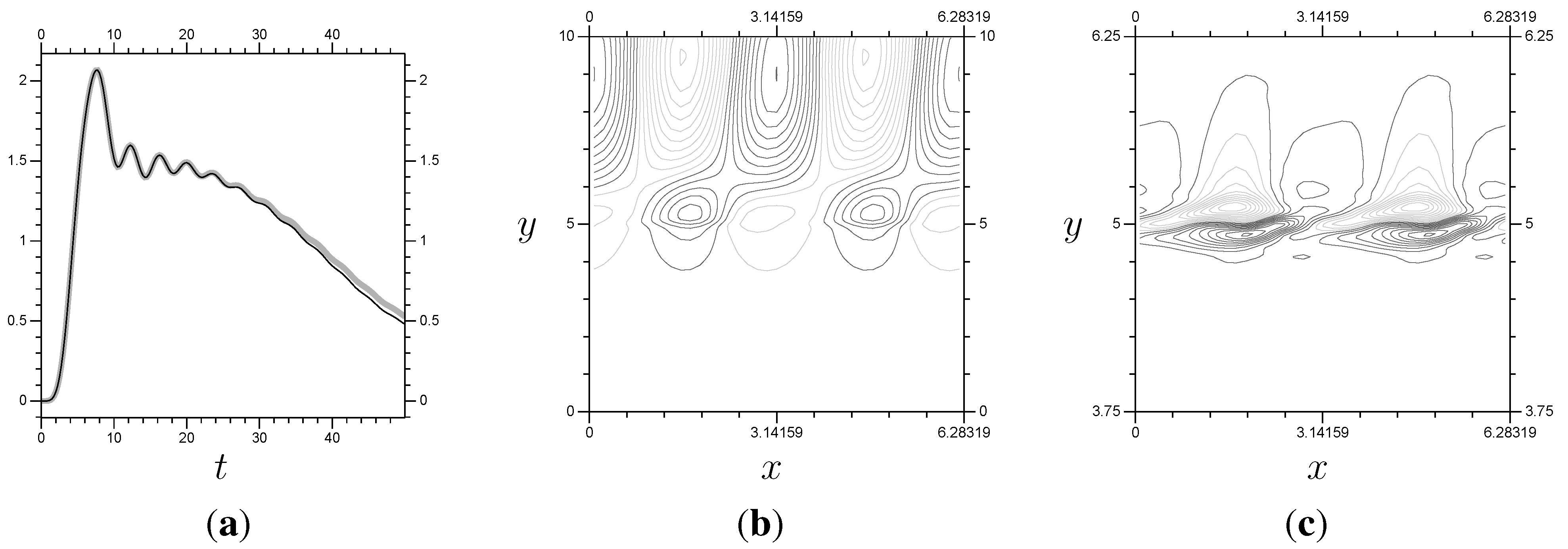
Now we discuss how this particular Rossby wave problem responds to the multi-scale method. The problem does seem to require a larger domain for the small-scale system, which cuts into the efficiency. The
system took an average of about 9.55 s per time step. See
Figure 16 for our multi-scale results with the smallest small-scale domain,
. The
double system requires approximately 3.51 s per time step, a significant improvement on the
system. However, the results are not quite as close to the
system as we would like. Including more elements above
improves things. In fact, the results are visually indistinguishable to the control results in
Figure 15. However, the
model requires 3.90 s per time step, and
requires 4.48 s per time step.
The multi-scale results were shown to be able to duplicate the results, using with a localized resolution. There was also a significant reduction in the effort, with the time step taking half as much time to compute. The resolution used was restricted to a coarse to keep computing requirements reasonable. The increase from to means that the small-scale system has approximately half of its coefficients be in , so coefficients that are also in the large-scale system. This is the least efficient form of the method, with only a single space worth of additional resolution in the small-scale system, and it still proved beneficial with the non-linear Rossby wave problem. The control results took about s per time step, while the, visually identical, multi-scale results with took 4.48 s per time step. So, we have accurate results with less than half the computational expense.
Figure 15.
Plots for the problem using . (Top) Flux; (Middle) P; (Bottom) Z. (a) P, ; (b) P, ; (c) P, ; (d) Z, ; (e) Z, ; (f) Z, .
Figure 15.
Plots for the problem using . (Top) Flux; (Middle) P; (Bottom) Z. (a) P, ; (b) P, ; (c) P, ; (d) Z, ; (e) Z, ; (f) Z, .
Figure 16.
Plots for
multi-scale models of the
Rossby wave problem. All use
. The flux is plotted against that for the
control results (the lighter, thicker line). The results using the larger
and
are omitted, as they are visually identical to the full
control results from
Figure 15. (
a)
; (
b)
P at
; (
c)
Z at
.
10.4. Convergence
The convergence of the Rossby wave problem is slightly restricted by the boundary conditions. Recall that the initial conditions are zero, while the
boundary condition is equal to
. Since Λ does not reach
, the boundary conditions are modeled at the large-scale resolution. The lack of resolution for the boundary conditions results in error that cannot be removed without significant modifications to the method (including a second small-scale system at
or incorporating the non-zero boundary conditions into Λ). As in the convergence related discussion in
Section 9, we look at the effect of different Λ sizes and “extra” terms on the accuracy of multi-scale results. The control results are a
resolution single system. The test systems use
or
over Ω and
on Λ. Plots of the
transformed error can be found in
Figure 17. The summarized data is in
Table 2.
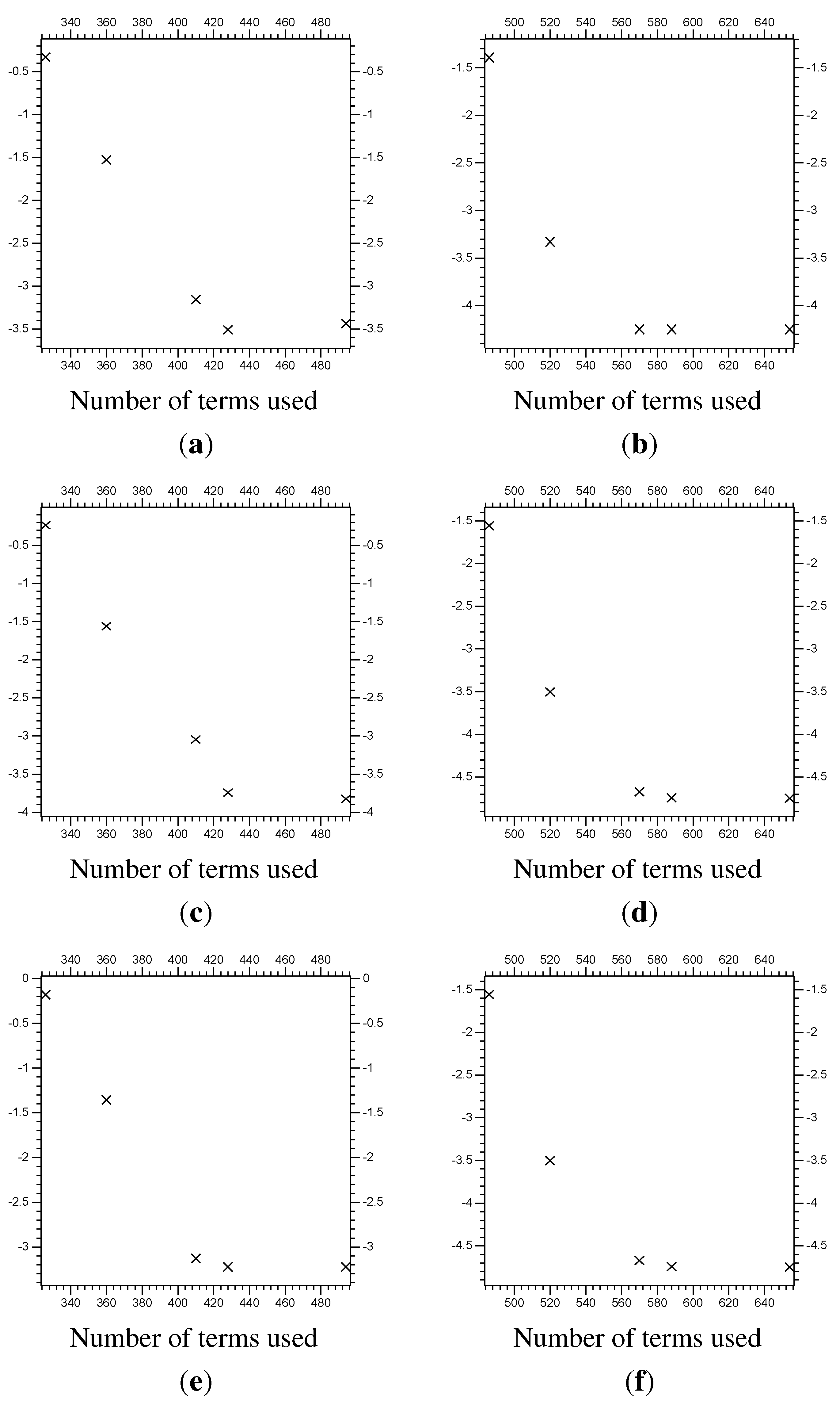
Now we take a look at the convergence from the non-linear results in
Section 10.3. The multi-scale results are calculated at
with
on differing small-scale domains Λ. They are compared with the full domain
control results. The usual plots of the error against the number of
and
coefficients used, and the time required, for the multi-scale system can be found in
Figure 18. The summarized data can be found in
Table 3.
Figure 17.
The error at of the function Z from the linear problem. The vertical axis is the of the error (the difference between the multi-scale system results and the control results). The horizontal axis is the total number of and coefficients used for the y directional decomposition. (a) of the error for with on Λ; (b) of the error for with on Λ; (c) of the error for with on Λ; (d) of the error for with on Λ; (e) of the error for with on Λ; (f) of the error for with on Λ.
Table 2.
Error from multi-scale linear Rossby wave results.
Table 2.
Error from multi-scale linear Rossby wave results.
| | Λ | “extra” | Terms | Error | Error | Error |
|---|
| [3.75,6.25] | 3 | 326 | | | |
| [3.50,6.50] | 4 | 360 | | | |
| [3.25,7.00] | 5 | 410 | | | |
| [3.00,7.00] | 6 | 428 | | | |
| [2.50,7.50] | 7 | 494 | | | |
| [3.75,6.25] | 3 | 486 | | | |
| [3.50,6.50] | 4 | 520 | | | |
| [3.25,7.00] | 5 | 570 | | | |
| [3.00,7.00] | 6 | 588 | | | |
| [2.50,7.50] | 7 | 654 | | | |
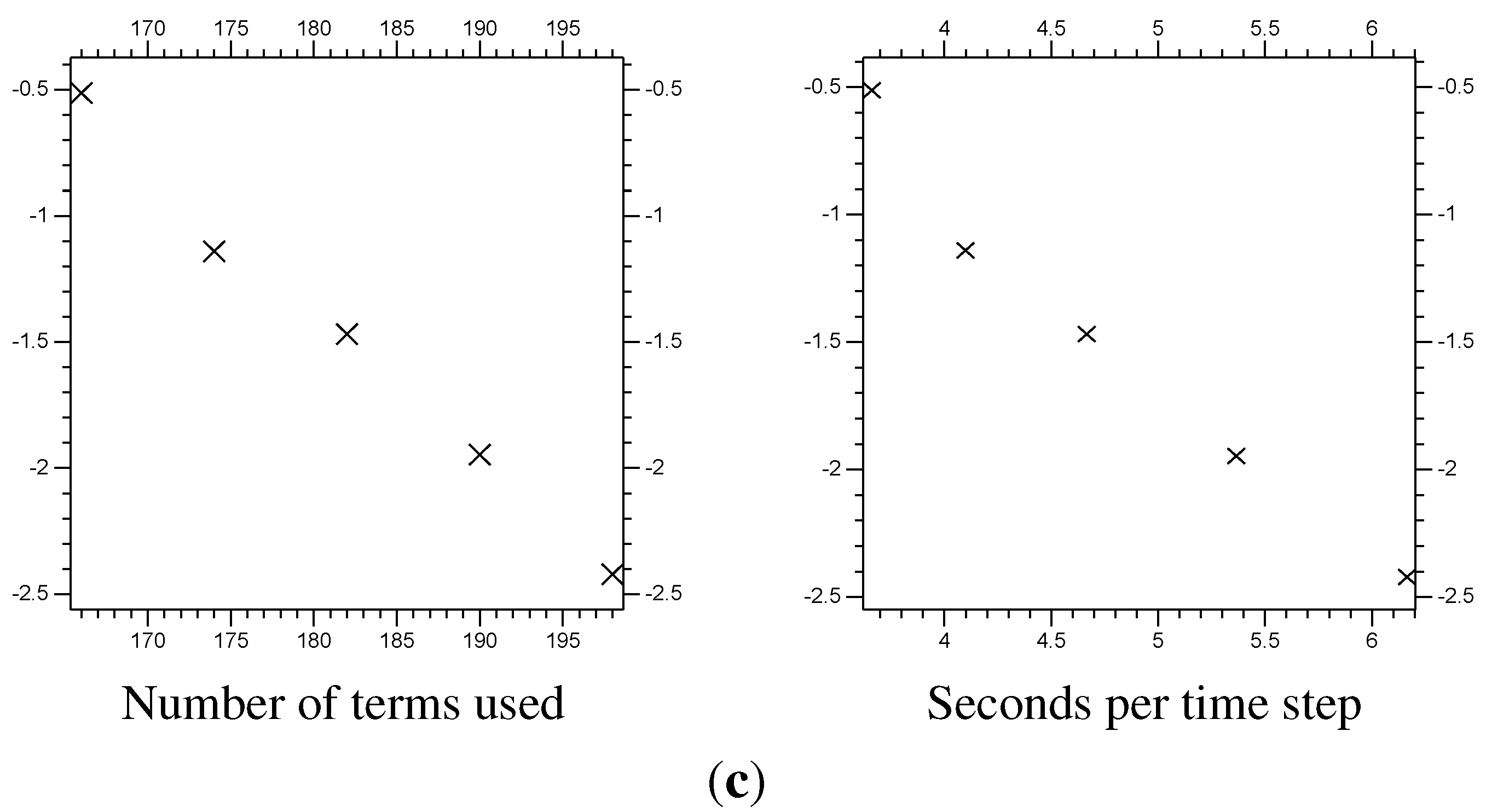
Figure 18.
The error at
of the function
Z from the non-linear (
) problem. The vertical axis is the
of the error, the difference between the
multi-scale results and the
control results (see
Figure 15). The horizontal axis is the total number of
and
coefficients used for the
y directional decomposition. (
a)
of the
error; (
b)
of the
error; (
c)
of the
error.
Table 3.
Error from non-linear multi-scale Rossby wave results. All but the control use and .
Table 3.
Error from non-linear multi-scale Rossby wave results. All but the control use and .
| Λ | “extra” | Terms | Time | Error | Error | Error |
|---|
| 4 | 168 | 3.66 | | | |
| 4 | 176 | 4.10 | | | |
| 4 | 184 | 4.67 | | | |
| 4 | 192 | 5.27 | | | |
| 4 | 200 | 6.16 | | | |
| Control | 9.25 | |
11. Conclusions
After some wavelet based preliminaries, we described a new method for partial differential equations at multiple scales, in
Section 3. The small-scale resolution is restricted to a sub-domain Λ of the full domain Ω. The method divides the implicit system created by the time-discretization scheme into two smaller systems: One at a coarse resolution over the entire domain Ω and the other at fine resolution on the subset
. This dividing of the system will typically result in significant computational savings.
Next we set up a test problem based on Burgers’ equation. The initial condition,
Figure 3a, results in two peaks that approach each other and collide. The resulting collision requires a fine resolution to be properly expressed. A resolution of
is required for stable and accurate results once the peaks collide (at approximately
). A resolution of
causes instability (coefficients in the range of
). However, since the collision is at
, the fine resolution is only required in a domain in the center. The calculations using a single resolution of
over the entire domain Ω take 0.988 s per time step. The resolution of
would be restricted to a sub-domain Λ in the center of Ω, where the peaks collide. The method required a few improvements beyond the basic setup, outlined in
Section 8.
We first tested the resolutions
on Ω and
on
, yielding a close approximation to the
control results. The largest
difference between them went briefly higher than 0.001, and otherwise was below 0.0005 (see
Figure 7). These differences were found to be an order of magnitude smaller than the error stemming from the limited resolution (
) and time step (
) common to both the multi-scale and control results (see
Subsection 7.3 and
Figure 4). Furthermore, the multi-scale results required 0.0337 s per time step, while the control results required approximately one second per time step. So, the multi-scale results were not only just stable and much less expensive to calculate, but also accurate.
The next step was to check for convergence towards the control results, computed using a resolution of on the full domain. For this test we used on Ω and on several different subsets Λ of Ω. We had to control for the error near the boundaries of Ω (far from the Λ sub-domains), which was, in fact, identical for all the different Λ sub-domains. Using the , and norms, increasing the size of the small-scale system resulted in a smaller difference between the test systems and the control results. The eventual error was approaching machine precision.
Next, further confirmation was sought using a non-trivial problem. The Rossby wave problem is two dimensional, on , with small-scale interactions found towards the center of the domain in the y direction. First we tested the linear form of the problem, where fine resolution near is needed to accurately represent the correct solution over time. Without viscosity, the numerical results would fail to maintain consistency beyond a certain value of t, with a finer resolution allowing this value of t to be larger. Using the linear problem with no viscosity, a wavelet decomposition with a resolution of will show the correct result over the time frame , over , and over . The multi-scale method was used with on and everywhere else, as well as a total of 6 “extra” terms. The results were accurate on , just like the full domain control results. So, the method worked for the linear version of the problem.
The non-linear Rossby wave problem also responded well to the multi-scale method. Similarly to the tests in
Section 9, a set of
with localized
were calculated, using different sub-domains Λ and different numbers of “extra” terms (see
Subsection 8.2). These were compared with full domain
control results. The
,
and
norms of the differences between the multi-scale and control results were calculated. As in
Section 9, the calculated differences between the test and control results showed a convergence to zero as the width of Λ was increased.
In
Section 8 two modifications to the basic method are introduced, one necessary for accurate results with a non-linear problem, the other contributing to accuracy for any problem. There are several additional features beyond those in
Section 8 that should be tested.
First is the fact that both the large and small-scale systems should have adaptive decompositions. Due to how the systems are divided, there is no particular reason why the small-scale system in Λ could not follow any given adaptive scheme (that is compatible with an implicit time-discretization). Most of the changes in an adaptive scheme would be towards the finer resolution terms, which interact very little with the large-scale system. The real question is how to determine if a particularly tight concentration of fine resolution terms merits creating further small-scale systems.
Giving the large-scale system an adaptive decomposition could be more complicated. Increasing the resolution of the large-scale system within Λ would probably be a bad idea. That would create duplicate terms (those that are calculated twice, once in each) to no net benefit. However, a few, isolated, small-scale calculations outside of Λ would obviously give greater accuracy, at limited expense. Again, the real question is when to decide that a set of small-scale terms would be best given its own small-scale system, and be calculated separately from the large-scale system.
Our two dimensional example involves a sub-domain Λ that covers a small subset of the domain in the y direction, but covers the entire interval in the x direction. Basically, the example has two spatial dimensions, but the multi-scale method is only used in one of those dimensions. It would be instructive to test a problem requiring localization in two or more spatial dimensions. A turbulence related problem would be appropriate for testing purposes, or any problem from fluid dynamics that results in small-scale vortices.
An analysis of the effect of our method on the stability of the underlying time-discretization. Preliminary testing was done in [
23], showing a minimal effect on stability, but more is needed.
Using multiple small-scale systems, either nested or discrete, as shown in
Figure 2. If a problem requires high resolution in two regions, call them
and
, it may be possible to calculate them separately, after the calculation of the large-scale system. The large-scale system could have, for example, 800 elements, with 400 small-scale elements and 200 large-scale in each of
and
. Solving all of these together would involve 1200 elements. Solving them broken up into three systems would involve an 800 element system and two of 400. This should involve substantial savings.
Using a different time step size for the small-scale system. Instead of calculating after each time step of the large-scale system, we could calculate then (or , , , then ). Doing so requires the intermediate large-scale vectors , which are relatively easy to calculate via interpolation. However, further experimentation is necessary to find how well this works, and what modifications may be necessary.
Making the size of Λ, the resolutions used, and the number of “extra” terms adaptive. This requires analyzing the sources of error stemming from the boundaries of Λ and the lack of “extra” terms.
Additionally, the key steps and components of this method could be combined with other methods. The method should be compatible with any multi-scale decomposition, and any procedures for solving the resulting systems. As long as the partial differential equation is time based, and the time-discretization is implicit, our multi-scale method should be useable. The nature of the partial differential equation itself will determine if our method would be useful.
So, in summary, this multi-scale implicit method shows potential for solving certain partial differential equations, namely those that produce stiff decompositions and require fine resolution in small regions. The preliminary tests went well, but further testing of the method, and extensions to the method, are required.


