
Construction and Analysis for the Optimal Supersaturated Designs with a Large Number of Inert Factors


1
School of Mathematics and Statistics, Qingdao University, Qingdao 266071, China
2
School of Mathematics and Computing Science, Guilin University of Electronic Technology, Guilin 541004, China
*
Authors to whom correspondence should be addressed.
Axioms 2024, 13(3), 179; https://doi.org/10.3390/axioms13030179
Submission received: 9 January 2024
/
Revised: 20 February 2024
/
Accepted: 6 March 2024
/
Published: 8 March 2024
Abstract
:Supersaturated designs (SSDs) refer to those designs in which the run size is much smaller than the main effects to be estimated. They are commonly used to identify a few, but critical, active factors from a large set of potentially active ones, keeping the cost as low as possible. In this regard, the development of new construction and analysis methods has recently seen a rapid increase. In this paper, we provide some methods to construct equi- and mixed-level optimal SSDs with a large number of inert factors using the substitution method. The proposed methods are easy to implement, and many new SSDs can then be constructed from them. We also study a variable selection method based on the screening-selection network (SSnet) method for regression problems. A real example is analyzed to illustrate that it is able to effectively identify active factors. Eight different analysis methods are used to analyze the data generated from the proposed designs. Three scenarios with different setups of parameters are designed, and the performances of each method are illustrated by extensive simulation studies. Among all these methods, SSnet produced the most satisfactory results according to power.
1. Introduction
In industry, it is often necessary to consider a large number of potentially relevant factors, of which only a small number are significant. However, due to practical restrictions, such as financial costs and time constraints, the actual number of test runs is often far from sufficient to estimate all potentially relevant factors, so the question of how to screen a small number of significant factors with a smaller number of tests becomes a critically important one. In this regard, supersaturated design (SSD), as a powerful tool for scenarios when the run size is much smaller than the main effects to be estimated, is used to reduce the cost of conducting experiments and to identify the active factors as correctly as possible. Therefore, the development of good supersaturated designs and variable screening methods are highly needed.
An SSD is fundamentally a fractional factorial design in which the number of potential effects is larger than the number of runs. Satterthwaite [1] was a pioneer who introduced the concept of SSDs in random balanced designs. Booth and Cox [2] conducted a comprehensive analysis of SSDs and introduced the criterion as a measure to evaluate 2-level SSDs. However, further research on such designs remained limited until Lin [3] and Wu [4]. They innovatively constructed SSDs by Hadamard matrices. With their potential in factor screening experiments, SSDs have gained growing popularity in recent years. Research on mixed-level SSDs has been extensive, with early contributions by Fang, Lin, and Liu [5,6], who introduced the criterion and the fractions of saturated orthogonal arrays (FSOA) method for efficiently constructing such designs. The evaluation of mixed-level SSDs has been approached by Yamada and Lin [7], who utilized the criterion. Fang et al. [6] further derived lower bounds and illustrated sufficient conditions to achieve the lower bounds. They demonstrated that both the and the criteria are special cases of criterion. Zou and Qin [8] provided new lower bounds of the criterion and the criterion. Consequently, this paper exclusively employs the criterion as the measure of choice. Georgiou, Koukouvinos, and Mantas [9] introduced a novel approach to constructing multi-level SSDs that are optimal under the criterion, utilizing resolvable balanced incomplete block designs. Thereafter, researchers have paid great attention to constructing mixed-level SSDs. Liu and Cai [10] presented a special substitution method, dividing the rows of a design into blocks and substituting the levels of another design with these blocks, yielding -optimal mixed-level SSDs. Sun, Lin, and Liu [11] achieved numerous optimal SSDs based on balanced designs and the construction of differential transposition, utilizing the Kronecker sum. For more details on the construction of SSDs, we refer to the works of Georgiou [12], Drosou and Koukouvinos [13], Jones et al. [14], Chatterjee and Koukouvinos [15], Khurana and Banerjee [16], Daraz et al. [17], Li et al. [18]. Further research is needed on the construction methods for -optimal SSDs with more flexible row and column numbers, especially in situations with a large number of inert factors.
The identification of active factors in SSDs poses a challenging problem, mainly attributed to the non-full rank and the potential for complex covariance between columns of the design matrix. Despite the existence of various methods for variable selection in factor screening experiments, a definitive optimal solution remains elusive. A prominent and widely used variable selection method is the least absolute shrinkage and selection operation (LASSO) [19], which effectively penalizes the squared loss of the data by incorporating an -norm penalty on the parameter vector. After LASSO was introduced, Fan and Li [20] introduced a class of variable selection procedures through nonconcave penalized likelihood, utilizing the smoothly clipped absolute deviation (SCAD) penalty. However, Li and Lin [21] demonstrated that direct application of the SCAD penalty for analyzing SSDs is not feasible due to the regularity conditions outlined in their paper, which necessitate a full rank design matrix. To address this limitation, Li and Lin [21] adopted the shrinkage estimation and the selection method proposed by Fan and Li [20], incorporating the SCAD penalty. They further extended the nonconcave penalized likelihood approaches to least squares, specifically focusing on scenarios where the design matrix is SSD. Zou [22] proposed a novel approach known as adaptive LASSO (Ada LASSO) in the context of finite parameters. It involves solving a convex optimization problem with an constraint, as described by Fan and Lv [23]. In another study, Candes and Tao [24] introduced the Dantzig selector (DS) method, which identifies the most relevant subset of variables or active factors by solving a straightforward convex program. Based on DS, Phoa, Pan, and Xu [25] conducted simulations to demonstrate the effectiveness of the DS method in analyzing SSDs, showcasing its superior efficiency compared to other approaches, such as the SCAD method elaborated by Das et al. [26]. The minimax concave penalty (MCP) method, introduced by Zhang [27], is highly advantageous as it ensures convexity in regions with low variable density while maintaining the desired thresholds for unbiasedness and variable selection. Drosou and Koukouvinos [28] proposed a novel method called support vector regression based on recursive feature elimination (SVR-RFE). This method is specifically designed to analyze SSDs for regression purposes; the method was shown to be efficient and accurate for two-level and mixed-level (two-level and three-level) SSDs. Errore et al. [29] assessed different model selection strategies and concluded that both the LASSO and the DS approach can successfully identify active factors. Ueda and Yamada [30] discussed the combination of SSDs and data analysis methods. In a pioneering contribution, Pokarowski et al. [31] introduced the screening-selection network (SSnet), an innovative approach that enhances the predictive power of LASSO by accommodating general convex loss functions. This novel method extends the applicability of LASSO beyond normal linear models, including logistic regression, quantile regression, and support vector machines. To effectively identify the most influential coefficients, the authors propose a novel technique where they meticulously order the absolute values of nonzero coefficients obtained through LASSO. Subsequently, the final model is selected from a small nested family using the generalized information criterion (GIC), ensuring optimal model performance. How the SSnet method performs in the analysis of equi- and mixed-level SSDs needs to be explored.
In order to evaluate the performance of the factor screening, we use power as the measure, which is defined by the proportion of active main effects successfully detected. This is extremely important because the use of SSDs is mainly to screen out the factors that should be considered for further investigation. The higher the power, the lower the probability of missing a truly active factor, which is more important in the case of SSDs. [13]
In this paper, we employ the substitution method, along with the generalized Hadamard matrix, to construct -optimal designs. Notably, the construction method can obtain more new equi- and mixed-level SSDs with a large number of inert factors. Meanwhile, the constructed designs possess the desirable characteristic of having no fully aliased columns. We also employ the SSnet method for analyzing SSDs for the first time. The results of the numerical study and real data analysis reveal that the SSnet method has a higher power than existing commonly used methods under different sparsity levels of effects. The SSnet method can be considered as an advantageous tool due to its extremely good performance in identifying active factors in SSDs.
The rest of the article is organized as follows. In Section 22, notation and definitions are introduced. In Section 33, supersaturated designs are extended to supersaturated designs in higher dimensions by the substitution method. In Section 44, we present the principles of the SSnet method and test whether it can select salient factors in variable selection. We also compare the power consumption of each variable selection method in SSD to validate the effectiveness of SSnet in this section. A conclusion is made in Section 5, where we discuss the most interesting findings of this paper.
2. Symbols and Definitions
A difference matrix is an matrix with entries from a finite Abelian group with s elements. It has the property that the vector difference between any two distinct columns, which is calculated by the addition operation on Abelian groups G, contains every element of G equally often (exactly times) [32]. For any difference matrix, if we subtract the first column from any column then we can obtain a normalized difference matrix. Its first column consists entirely of the zero element of G [33]. A matrix M is called a generalized Hadamard matrix if and only if both M and its transposition are difference matrices. We denote a normalized generalized Hadamard matrix used in this paper as , which is a array with s elements, and its first column consists entirely of . For any prime power, s, and integers , theorem 6.6 of Hedayat et al. [33] shows the generalized Hadamard matrix exists. Lemma 3 of Li et al. [18] provides the construction method of the generalized Hadamard matrix . A generalized Hadamard matrix based on Galois field is shown below, where the vector difference between any two columns contains and 2 equally often.
A mixed-level design, , has n runs and m factors with levels, respectively, where the -level is taken from a set of symbols, . When , D is called a saturated design, and when , it is called a supersaturated design. When some ’s are equal, we use the notation , indicating factors having levels, . If all the ’s are equal, the design is said to be equi-level and denoted by . A design is called balanced if each column has the equal occurrence property of the symbols. Throughout this paper, we only consider balanced designs.
For a design consisting of , we assume that the ith column, , and the jth column, , have a level and a level, respectively. The criterion is defined as
where , , is the number of -pairs in , and stands for the average frequency of level-combinations in . Here, the subscript “NOD” stands for nonorthogonality of the design. The value provides a nonorthogonality measure for . Thus, measures the average nonorthogonality among the columns of D. If and only if , the and columns are orthogonal. If and only if , the design is orthogonal, that is, for any .
Let be the coincidence number between rows h and l, which is defined to be the number of k’s, such that . Fang et al. [34] expressed as
where , the lower bound of which is
where denotes the integer part of ,
Note that when , . They present a sufficient condition for a design being -optimal.
Lemma 1.
If the difference among all coincidence numbers between distinct rows of design D does not exceed one, then D is -optimal.
A design with equal coincidence numbers between different rows is called an equidistant design. We know that equidistant designs are -optimal designs. In the whole paper, we use the criterion.
3. Generation of SSDs by Substitution Method
In this section, the generalized Hadamard matrix is extended to SSDs with a large number of inert factors using a special substitution method.
Let A be a matrix with a cyclic structure denoted as , where . The elements in the first row are all 0 and the second row is . Each remaining row of this matrix is obtained from each previous row by moving the first element to the last position and cyclicly permutating the other elements to the left. It is obvious that the coincidence number of A is zero.
Construction 1.
Step 1. Let A be the design .
Step 2. Let B be the design obtained by ignoring the first column (all-zero column) of the generalized Hadamard matrix , which is an equidistant design also denoted as .
Step 3. Substitute the ith level of B by the ith row of A, , respectively.
Step 4. We obtain a new design P, denoted by .
Theorem 1.
The new design, , obtained by Construction 1 is an -optimal design.
Proof of Theorem 1.
Since the transposition of the generalized Hadamard matrix is a difference matrix, the number 0 occurs times in the vector difference between any two different rows of . It is natural that the coincidence numbers of B and A in Construction 1 take the constant , , respectively. P is obtained via substituting the ith level of B by the ith row of A. For any two rows of h and l of B, the same level is substituted by the same row of A, so the coincidence number of these is . The different levels are substituted by the different rows of A, so the coincidence number of these is 0 because of . Therefore, the coincidence number of the generated design P is , which is the product of the factors of A and the coincidence number of B. We know that the design is -optimal when the coincidence number is a constant. Thus, P is an -optimal design. □
Specifically, when B is also in Construction 1, the -optimal design can be obtained by the substitution method with the coincidence number of 0.
Example 1.
Construction 2.
Step 1. Let A be the design . Let be the design obtained by Construction 1.
Step 2. For , let .
Step 3. Substitute the ith level of by the ith row of A.
Step 4. We obtain a new design, , denoted by .
Step 5. Repeat Steps 2–4 until the required number of columns is reached.
Corollary 1.
For , the new design obtained by Construction 2 is an -optimal design.
Proof of Corollary 1.
The coincidence numbers of and A in Construction 2 take the constant , , respectively. The coincidence number of the generated design is , which is the product of the factors of A and the coincidence number of . Thus, is an -optimal design. □
Lemma 2
(Li et al. [18], Corollary 1). If s is a prime power, the generalized Hadamard matrix can be constructed by Lemma 3(ii) or Remark 2, then (where is the Kronecker sum defined on the Abelian group G) is a generalized Hadamard matrix, .
By deleting the first column of , we can obtain the -optimal design , and it is an equidistant design.
Construction 3.
Step 1. Let A be the design .
Step 2. Let B be obtained by Lemma 2.
Step 3. Substitute the ith level of B by the ith row of A, respectively.
Step 4. We obtain a new design P, denoted by .
Theorem 2.
The new design obtained by Construction 3 is an -optimal design.
Proof of Theorem 2.
The coincidence number of A is and the coincidence number of B is . Now consider the coincidence number between any two distinct rows of h and l of the generated design P is a constant , so P is -optimal. □
Example 2.
In the above theorems, there is a strict limitation that design B and the -optimal designs that can be constructed are all equi-level SSDs. We now introduce two methods for constructing -optimal mixed-level SSDs.
Lemma 3
(Fang et al. [6], Theorem 4). Let X be a saturated orthogonal array, , and be a prime power, and let , , ; the -optimal mixed-level supersaturated design is obtained from and the level factor is orthogonal to the q level factor, and it is also an equidistant design.
Construction 4.
Step 1. Let A be the design .
Step 2. Let B be obtained by Lemma 3, where and is the lowest common multiple of p and q, . Divide B into s sub-designs by rows; these sub-designs are denoted by , each with rows and m columns.
Step 3. Substitute the ith level of A by the ith sub-design of B, respectively.
Step 4. We obtain a new design P denoted by .
Theorem 3.
The new design obtained by Constructon 4 is an -optimal SSD.
Proof of Theorem 3.
The coincidence number between any two rows is a constant, ; thus, D is -optimal. □
Example 3.
Example 4.
Construction 5.
Step 1. Let A be the design .
Step 2. Let B be the () in Corollary 3 of Li et al. [18], which can be denoted by , where q is a prime power, . D is the design obtained by deleting the first columns of in Lemma 2. Divide D into sub-designs by columns, and is the -th sub-design, . F is an equidistant design with a constant coincidence number λ. . Divide B into s sub-designs by rows.
Step 3. Substitute the ith level of A by the ith sub-design of B, respectively.
Step 4. We obtain a new design P denoted by
.
Theorem 4.
If . The new design P obtained by Construction 5 is an -optimal SSD.
Proof of Theorem 4.
When , design B is an equidistant design with a constant coincidence number, . The coincidence number of design P is a constant , so it is optimal. □
Example 5.
In fact, using the similar method of Construction 2, we can further expand Constructions 3–5 to obtain more new SSDs with flexible columns.
Corollary 2.
Since the B designs in Constructions 3–5 have no completely aliased columns, the generated designs constructed by the above construction methods have no completely aliased columns.
Actually, most B designs in Construction 1 have no completely aliased columns, and the generated design constructed by Constructions 1 and 2 have no completely aliased columns.
Proof of Corollary 2.
Let be the i-th column of design and be the l-th sub-design of design B. Then the value between and is . Where , , , and . It is easy to find that the for generating design P is determined by the of B. Because B performs well in its maximum value , there is no fully aliased column in the generated design P. □
In this section, we provided five construction methods to obtain many new equi- and mixed-level SSDs with a large number of inert factors by the substitution method. The proposed methods are easy to implement and most obtained SSDs have no fully aliased columns.
4. Variable Selection Method for SSD
For the problem of variable selection in SSDs, there remains a significant challenge. In this section, to facilitate a comprehensive comparison of variable selection methods for active factor identification on SSDs, a novel variable selection method, SSnet, is first used to perform factor screening on the Williams Rubber dataset, comparing it to seven other widely recognized and applicable methods for SSDs. These methods include Lq-penalty, Ada LASSO [22], SCAD [21], MCP [27], Ds [25], SVR-RFE [28], and ISIS [13]. This was done in order to validate the effectiveness and rationality of SSnet in factor identification. Then, through simulations, the constructed SSDs are used as simulated data to compare these seven different variable selection methods and provide power values for different scenarios of the active factor quantities. We conclude that SSnet has a strong ability to identify active factors on SSDs.
4.1. SSnet
Pokarowski et al. [31] introduced an innovative approach aimed at enhancing the performance of the LASSO method in predictive models with convex loss functions. This method involves systematically ordering the nonzero coefficients of the LASSO based on their absolute values under a specific penalty. Subsequently, the final model is selected from a compact nested family using GIC.
The SS algorithm employs two selection procedures for variable selection. Firstly, the TL method extracts only the absolute values of the LASSO estimator for variables surpassing a specific threshold. The second step, termed the SS procedure, identifies the minimum GIC value among nested families constructed using sequences comprising nonzero LASSO coefficients. Fundamentally, the SS algorithm can be viewed as a GIC-based LASSO approach with adaptive thresholding. To practically implement the SS algorithm, the SSnet algorithm utilizes the R package to calculate LASSO values across a range of penalty values. Subsequently, the optimal model is selected from a small family by minimizing the GIC.
In this paper, we demonstrate the applicability of the SSnet-based variable selection method to SSDs. We assess its performance through real-world examples and simulations and compare it with other popular methods without making general claims.
4.2. Practical Example
This example utilizes an SSD constructed by Lin [3] and the rubber data obtained from Williams [35]. The SSD presented in Table 4 is employed in this study. The design consists of 24 factors and 14 runs. However, as it contains two identical columns, namely 13 and 16, one of them needs to be eliminated. Consequently, the final analysis will retain the remaining 23 factors. In this case, column 13, corresponding to the 13-factor, was selected for deletion. Additionally, the labels of factors 14–24 were amended to 13–23.
The original analysis was based on Williams’ study of a 28-trial versus 24-factor Plackett–Burma design. The rubber data have been previously scrutinized by numerous researchers, including Abraham, Chipman, and Vijayan [36], who employed full subset regression to narrow down the search for the optimal subset within a model with five or fewer factors; Bettie, Fong, and Lin [37], who compared various model selection methods; Li and Lin [38], who adopted a stepwise SCAD approach; and Phoa et al. [25], who introduced the DS method. In this study, the SSnet algorithm is utilized to investigate this two-level supersaturated design. A concise summary of the analysis of the rubber data in each model is presented in Table 4, displaying the respective sizes and variables for each method, as well as the selected model.
The presence of factor 14 in all selected models highlights its significance, making it a noteworthy factor in the SSD. Comparing the various methods used, it becomes evident that SSnet efficiently identifies a significant set of factors while maintaining a smaller model size. This serves as solid evidence for the soundness and accuracy of the SSnet method to variable selection.
4.3. Simulation
To compare the performance of the proposed SSnet method with the other five methods, we generate data from a unique main effects linear model, , with X being an SSD matrix, and a random error, , ; y is the observed data. We consider two factor models: of the active factor is generated by , with an absolute value of 2 or 5 for , and of the other inactive factors equal to 0. To demonstrate the performance of various methods in screening active factors under different sparsity levels, the three scenarios are used based on the number of active factors. Experience has shown that the number of runs used in the screening design should be at least twice the number of potentially significant effects. Therefore, the maximum number of active factors is set to be . The analysis of SSDs is based on the principle of sparse effects [39]. This principle advocates that relatively few of the effects studied in the screening design are active, so the number of active factors in the effect sparse scenario is set to be less than the of (). The number of active factors in the intermediate complexity scenario is between the of () and the of (). Meanwhile, this selection and construction of three scenarios is similar to the setting of Marley and Woods [40] and Drosou and Koukouvinos [13,28], which makes it convenient to compare with methods in existing papers. The active factors are randomly selected from X and the number of that is set according to the following scenarios:
- Scenario I (Effect sparse scenario): .
- Scenario II (Moderately complex scenarios): .
- Scenario III (Massive effect scenario): .
The number of active factor for Scenario I is taken as , with each quantity of active factors simulated 1000 times and averaged. We use Mean power to represent the overall average of the corresponding power under each quantity of active factors. Similarly, for Scenario II, take , and for Scenario III, take . Without loss of generality, we select three different SSDs as the input matrix in this section, shown respectively as Examples 2, 4, and 5.
Example 6.
In this example, we choose the generated design of Example 2 as the input SSD matrix X. We choose the number of active factors to be 1∼6, 7∼9, and 10∼18 in three different scenarios, respectively.
Figure 1 shows the mean power of SSD in various scenarios. Model 1 is a model with random coefficients of small magnitude equal to 2 and variance equal to 1. This leads to a more complicated model with coefficients as small as the error term. Model 2 is a model with random coefficients but with relatively large magnitude equal to 5 and variance equal to 1.
Scenario I.
In Model 1, SSnet shows the highest mean power of approximately 97%; SCAD, Lq-penalty, MCP, Ds, ISIS, and Ada LASSO have almost the same mean power of approximately 90%; while SVR-RFE performs poorly with a mean power of 85%. Similarly, SSnet in Model 2 shows excellent performance, with mean power almost reaching 1; other methods have also reached over 95%. These figures indicate that the reliability of these methods is consistently high, even when the activity factors are sparse.
Scenario II.
Similar to Scenario I, SSnet exhibits the highest mean power in this scenario. In Model 1, only the mean power of SSnet and SCAD reached 90%, followed by MCP, DS, and ISIS, with a mean power above 85%, and Lq-penalty, Ada LASSO, and SVR-RFE, with a mean power around 80%. In Model 2, SSnet shows the highest mean power of approximately 98%; the other methods, except for ISIS, had a mean power above 90%. It is evident that SSnet dominates among these eight methods in moderately complex situations.
Scenario III.
In massive effect scenarios, the differences between each method are more significant, exhibiting different mean power levels. SSnet stands out, with a significantly higher mean power compared to the other methods.
In Example 6, SSnet demonstrated excellent factor screening ability on equi-level SSDs. Next, we will continue to use mixed-level SSDs to enhance the persuasiveness of this conclusion.
Example 7.
In this example, the generation design of Example 3 is considered as the input SSD matrix. We choose the number of active factors to be 1∼2, 3, and 4∼6 in three different scenarios for the two models, respectively. The results, focusing on mean power, are shown in Figure 2.
In Scenario I, SSnet has the highest mean power, with only SSnet achieving a mean power value of 90% in Model 1, and SSnet approaching 1 in Model 2. In both Scenario II and Scenario III, SSnet performed the best in terms of mean power. In this example, the mean power of SSnet is optimal, significantly surpassing other methods.
From Example 7, it can be seen that SSnet has a significant ability to identify active factors on mixed-level SSDs. Let us further verify this conclusion.
Example 8.
In this example, consider the generated design of Example 5 as the input SSD matrix. We choose the number of active factors to be 1∼6, 7∼9, and 10∼18 in three different scenarios for both models; the results, focusing on mean power, are shown in Figure 3.
It is clear that Model 1 always exhibits lower mean power than Model 2, indicating that the model with larger random coefficients is more capable of recognizing in scenarios with sparse active factors. SSnet always has the highest average power in scenes 2 and 3. Although Lq-penalty has a slightly higher average power than SSnet in Scenario I, its mean power in Scenarios II and III decreases significantly, especially in Scenario III, which is only 30%, which is very unstable. On the other hand, SSnet has a high mean power in all scenarios and is robust.
In conclusion, whether in equi-level design or mixed-level SSDs, the ability of SSnet to identify active factors has been proven to be robust, maintaining consistently high mean power across all scenarios. It is evident that SSnet is particularly sensitive to random coefficients. It performs better in scenarios where active factors are sparse in SSDs and where there are larger random coefficients.
5. Conclusions
SSDs are commonly used to select a small number of active factors from a large number of candidates. In this paper, many new equi- and mixed-level SSDs with a large number of inert factors are constructed by the substitution method of the generalized Hadamard matrix, and most SSDs have no fully aliased columns. The proposed methods are easy to implement and the number of columns is more flexible. These SSDs can serve as a good check when identifying active factors using variable selection methods. Note that the substitution method can generate large designs using small equidistant designs. Changing the source small design to other types of design can result in more SSDs or other space-filling designs, which is worthy of further study. This paper investigates the application of SSnet as a model selection method in SSDs, marking its novelty as it is employed for the first time in this context. The main emphasis during screening tests lies in accurately identifying valid effects rather than excluding invalid ones, focusing primarily on power. The major advantage of SSnet lies in its capacity to deliver robust performance against power in SSDs despite its simplicity. Simulation studies have consistently demonstrated that SSnet produces excellent outcomes and can be meaningfully compared with the existing analysis methods proposed in the literature. Additionally, it demonstrates exceptional performance, not only in scenarios with extremely sparse real models but also in cases with moderately active effects. Furthermore, this approach exhibits the capability to effectively handle large-scale designs comprising numerous factors, including both equi- and mixed-level designs.
Author Contributions
Conceptualization, M.L. and X.H.; methodology, M.L. and X.W.; software, X.W. and X.H.; validation, W.Z.; formal analysis, M.L and X.W.; investigation, W.Z.; resources, M.L.; data curation, X.H.; writing—original draft preparation, X.H. and M.L.; writing—review and editing, M.L. and X.W.; visualization, X.W.; supervision, W.Z.; project administration, M.L. All authors have read and agreed to the published version of the manuscript.
Funding
This research was funded by the Shandong Provincial Natural Foundation of China (ZR2021QA053, ZR2021QA044) and the National Natural Science Foundation of China (12101346).
Data Availability Statement
Data are contained within the article.
Conflicts of Interest
The authors declare no conflicts of interest.
Appendix A

Table A1.
.
| 1 | 2 | 3 | 4 | |
|---|---|---|---|---|
| 1 | 0 | 0 | 1 | 2 |
| 2 | 0 | 1 | 2 | 0 |
| 3 | 0 | 2 | 0 | 1 |
| 4 | 1 | 0 | 2 | 1 |
| 5 | 1 | 1 | 0 | 2 |
| 6 | 1 | 2 | 1 | 0 |
Table A2.
.
| 1 | 2 | 3 | 4 | 5 | |
|---|---|---|---|---|---|
| 1 | 0 | 0 | 0 | 0 | 0 |
| 2 | 1 | 2 | 3 | 4 | 5 |
| 3 | 2 | 3 | 4 | 5 | 1 |
| 4 | 3 | 4 | 5 | 1 | 2 |
| 5 | 4 | 5 | 1 | 2 | 3 |
| 6 | 5 | 1 | 2 | 3 | 4 |
Table A3.
.
| 1 | 2 | 3 | 4 | 5 | 6 | 7 | 8 | 9 | 10 | 11 | 12 | 13 | 14 | 15 | 16 | 17 | 18 | 19 | 20 | |
|---|---|---|---|---|---|---|---|---|---|---|---|---|---|---|---|---|---|---|---|---|
| 1 | 0 | 0 | 1 | 2 | 0 | 0 | 1 | 2 | 0 | 0 | 1 | 2 | 0 | 0 | 1 | 2 | 0 | 0 | 1 | 2 |
| 2 | 0 | 1 | 2 | 0 | 0 | 2 | 0 | 1 | 1 | 0 | 2 | 1 | 1 | 1 | 0 | 2 | 1 | 2 | 1 | 0 |
| 3 | 0 | 2 | 0 | 1 | 1 | 0 | 2 | 1 | 1 | 1 | 0 | 2 | 1 | 2 | 1 | 0 | 0 | 1 | 2 | 0 |
| 4 | 1 | 0 | 2 | 1 | 1 | 1 | 0 | 2 | 1 | 2 | 1 | 0 | 0 | 1 | 2 | 0 | 0 | 2 | 0 | 1 |
| 5 | 1 | 1 | 0 | 2 | 1 | 2 | 1 | 0 | 0 | 1 | 2 | 0 | 0 | 2 | 0 | 1 | 1 | 0 | 2 | 1 |
| 6 | 1 | 2 | 1 | 0 | 0 | 1 | 2 | 0 | 0 | 2 | 0 | 1 | 1 | 0 | 2 | 1 | 1 | 1 | 0 | 2 |
Table A4.
.
| 1 | 2 | 3 | 4 | 5 | |
|---|---|---|---|---|---|
| 1 | 0 | 0 | 0 | 0 | 0 |
| 2 | 0 | 1 | 1 | 1 | 1 |
| 3 | 0 | 2 | 2 | 2 | 2 |
| 4 | 0 | 3 | 3 | 3 | 3 |
| 5 | 1 | 3 | 0 | 2 | 1 |
| 6 | 1 | 1 | 2 | 0 | 3 |
| 7 | 1 | 2 | 1 | 3 | 0 |
| 8 | 1 | 0 | 3 | 1 | 2 |
| 9 | 2 | 0 | 1 | 2 | 3 |
| 10 | 2 | 3 | 2 | 1 | 0 |
| 11 | 2 | 1 | 0 | 3 | 2 |
| 12 | 2 | 2 | 3 | 0 | 1 |
Table A5.
.
| 1 | 2 | 3 | 4 | 5 | 6 | 7 | 8 | 9 | 10 | 11 | |
|---|---|---|---|---|---|---|---|---|---|---|---|
| 1 | 0 | 0 | 0 | 0 | 0 | 0 | 0 | 0 | 0 | 0 | 0 |
| 2 | 1 | 2 | 3 | 4 | 5 | 6 | 7 | 8 | 9 | 10 | 11 |
| 3 | 2 | 3 | 4 | 5 | 6 | 7 | 8 | 9 | 10 | 11 | 1 |
| 4 | 3 | 4 | 5 | 6 | 7 | 8 | 9 | 10 | 11 | 1 | 2 |
| 5 | 4 | 5 | 6 | 7 | 8 | 9 | 10 | 11 | 1 | 2 | 3 |
| 6 | 5 | 6 | 7 | 8 | 9 | 10 | 11 | 1 | 2 | 3 | 4 |
| 7 | 6 | 7 | 8 | 9 | 10 | 11 | 1 | 2 | 3 | 4 | 5 |
| 8 | 7 | 8 | 9 | 10 | 11 | 1 | 2 | 3 | 4 | 5 | 6 |
| 9 | 8 | 9 | 10 | 11 | 1 | 2 | 3 | 4 | 5 | 6 | 7 |
| 10 | 9 | 10 | 11 | 1 | 2 | 3 | 4 | 5 | 6 | 7 | 8 |
| 11 | 10 | 11 | 1 | 2 | 3 | 4 | 5 | 6 | 7 | 8 | 9 |
| 12 | 11 | 1 | 2 | 3 | 4 | 5 | 6 | 7 | 8 | 9 | 10 |
Table A6.
.
| 1 | 2 | 3 | 4 | 5 | 6 | 7 | 8 | 9 | 10 | 11 | 12 | 13 | 14 | 15 | 16 | 17 | 18 | 19 | 20 | 21 | 22 | 23 | 24 | 25 | 26 | 27 | 28 | 29 | 30 | 31 | 32 | 33 | 34 | 35 | |
|---|---|---|---|---|---|---|---|---|---|---|---|---|---|---|---|---|---|---|---|---|---|---|---|---|---|---|---|---|---|---|---|---|---|---|---|
| 1 | 0 | 0 | 0 | 0 | 0 | 0 | 0 | 0 | 0 | 0 | 0 | 0 | 0 | 0 | 0 | 0 | 0 | 0 | 0 | 0 | 0 | 0 | 0 | 0 | 0 | 0 | 0 | 0 | 0 | 0 | 0 | 0 | 0 | 0 | 0 |
| 2 | 1 | 2 | 1 | 2 | 0 | 0 | 1 | 2 | 1 | 2 | 0 | 0 | 1 | 2 | 1 | 2 | 0 | 0 | 1 | 2 | 1 | 2 | 0 | 0 | 1 | 2 | 1 | 2 | 0 | 0 | 1 | 2 | 1 | 2 | 0 |
| 3 | 2 | 1 | 1 | 0 | 2 | 0 | 2 | 1 | 1 | 0 | 2 | 0 | 2 | 1 | 1 | 0 | 2 | 0 | 2 | 1 | 1 | 0 | 2 | 0 | 2 | 1 | 1 | 0 | 2 | 0 | 2 | 1 | 1 | 0 | 2 |
| 4 | 2 | 2 | 0 | 1 | 1 | 0 | 2 | 2 | 0 | 1 | 1 | 0 | 2 | 2 | 0 | 1 | 1 | 0 | 2 | 2 | 0 | 1 | 1 | 0 | 2 | 2 | 0 | 1 | 1 | 0 | 2 | 2 | 0 | 1 | 1 |
| 5 | 0 | 1 | 2 | 2 | 1 | 0 | 0 | 1 | 2 | 2 | 1 | 0 | 0 | 1 | 2 | 2 | 1 | 0 | 0 | 1 | 2 | 2 | 1 | 0 | 0 | 1 | 2 | 2 | 1 | 0 | 0 | 1 | 2 | 2 | 1 |
| 6 | 1 | 0 | 2 | 1 | 2 | 0 | 1 | 0 | 2 | 1 | 2 | 0 | 1 | 0 | 2 | 1 | 2 | 0 | 1 | 0 | 2 | 1 | 2 | 0 | 1 | 0 | 2 | 1 | 2 | 0 | 1 | 0 | 2 | 1 | 2 |
| 7 | 0 | 0 | 0 | 0 | 0 | 1 | 1 | 1 | 1 | 1 | 1 | 2 | 2 | 2 | 2 | 2 | 2 | 1 | 1 | 1 | 1 | 1 | 1 | 2 | 2 | 2 | 2 | 2 | 2 | 0 | 0 | 0 | 0 | 0 | 0 |
| 8 | 1 | 2 | 1 | 2 | 0 | 1 | 2 | 0 | 2 | 0 | 1 | 2 | 0 | 1 | 0 | 1 | 2 | 1 | 2 | 0 | 2 | 0 | 1 | 2 | 0 | 1 | 0 | 1 | 2 | 0 | 1 | 2 | 1 | 2 | 0 |
| 9 | 2 | 1 | 1 | 0 | 2 | 1 | 0 | 2 | 2 | 1 | 0 | 2 | 1 | 0 | 0 | 2 | 1 | 1 | 0 | 2 | 2 | 1 | 0 | 2 | 1 | 0 | 0 | 2 | 1 | 0 | 2 | 1 | 1 | 0 | 2 |
| 10 | 2 | 2 | 0 | 1 | 1 | 1 | 0 | 0 | 1 | 2 | 2 | 2 | 1 | 1 | 2 | 0 | 0 | 1 | 0 | 0 | 1 | 2 | 2 | 2 | 1 | 1 | 2 | 0 | 0 | 0 | 2 | 2 | 0 | 1 | 1 |
| 11 | 0 | 1 | 2 | 2 | 1 | 1 | 1 | 2 | 0 | 0 | 2 | 2 | 2 | 0 | 1 | 1 | 0 | 1 | 1 | 2 | 0 | 0 | 2 | 2 | 2 | 0 | 1 | 1 | 0 | 0 | 0 | 1 | 2 | 2 | 1 |
| 12 | 1 | 0 | 2 | 1 | 2 | 1 | 2 | 1 | 0 | 2 | 0 | 2 | 0 | 2 | 1 | 0 | 1 | 1 | 2 | 1 | 0 | 2 | 0 | 2 | 0 | 2 | 1 | 0 | 1 | 0 | 1 | 0 | 2 | 1 | 2 |
| 13 | 0 | 0 | 0 | 0 | 0 | 2 | 2 | 2 | 2 | 2 | 2 | 1 | 1 | 1 | 1 | 1 | 1 | 1 | 1 | 1 | 1 | 1 | 1 | 0 | 0 | 0 | 0 | 0 | 0 | 2 | 2 | 2 | 2 | 2 | 2 |
| 14 | 1 | 2 | 1 | 2 | 0 | 2 | 0 | 1 | 0 | 1 | 2 | 1 | 2 | 0 | 2 | 0 | 1 | 1 | 2 | 0 | 2 | 0 | 1 | 0 | 1 | 2 | 1 | 2 | 0 | 2 | 0 | 1 | 0 | 1 | 2 |
| 15 | 2 | 1 | 1 | 0 | 2 | 2 | 1 | 0 | 0 | 2 | 1 | 1 | 0 | 2 | 2 | 1 | 0 | 1 | 0 | 2 | 2 | 1 | 0 | 0 | 2 | 1 | 1 | 0 | 2 | 2 | 1 | 0 | 0 | 2 | 1 |
| 16 | 2 | 2 | 0 | 1 | 1 | 2 | 1 | 1 | 2 | 0 | 0 | 1 | 0 | 0 | 1 | 2 | 2 | 1 | 0 | 0 | 1 | 2 | 2 | 0 | 2 | 2 | 0 | 1 | 1 | 2 | 1 | 1 | 2 | 0 | 0 |
| 17 | 0 | 1 | 2 | 2 | 1 | 2 | 2 | 0 | 1 | 1 | 0 | 1 | 1 | 2 | 0 | 0 | 2 | 1 | 1 | 2 | 0 | 0 | 2 | 0 | 0 | 1 | 2 | 2 | 1 | 2 | 2 | 0 | 1 | 1 | 0 |
| 18 | 1 | 0 | 2 | 1 | 2 | 2 | 0 | 2 | 1 | 0 | 1 | 1 | 2 | 1 | 0 | 2 | 0 | 1 | 2 | 1 | 0 | 2 | 0 | 0 | 1 | 0 | 2 | 1 | 2 | 2 | 0 | 2 | 1 | 0 | 1 |
| 19 | 0 | 0 | 0 | 0 | 0 | 2 | 2 | 2 | 2 | 2 | 2 | 2 | 2 | 2 | 2 | 2 | 2 | 0 | 0 | 0 | 0 | 0 | 0 | 1 | 1 | 1 | 1 | 1 | 1 | 1 | 1 | 1 | 1 | 1 | 1 |
| 20 | 1 | 2 | 1 | 2 | 0 | 2 | 0 | 1 | 0 | 1 | 2 | 2 | 0 | 1 | 0 | 1 | 2 | 0 | 1 | 2 | 1 | 2 | 0 | 1 | 2 | 0 | 2 | 0 | 1 | 1 | 2 | 0 | 2 | 0 | 1 |
| 21 | 2 | 1 | 1 | 0 | 2 | 2 | 1 | 0 | 0 | 2 | 1 | 2 | 1 | 0 | 0 | 2 | 1 | 0 | 2 | 1 | 1 | 0 | 2 | 1 | 0 | 2 | 2 | 1 | 0 | 1 | 0 | 2 | 2 | 1 | 0 |
| 22 | 2 | 2 | 0 | 1 | 1 | 2 | 1 | 1 | 2 | 0 | 0 | 2 | 1 | 1 | 2 | 0 | 0 | 0 | 2 | 2 | 0 | 1 | 1 | 1 | 0 | 0 | 1 | 2 | 2 | 1 | 0 | 0 | 1 | 2 | 2 |
| 23 | 0 | 1 | 2 | 2 | 1 | 2 | 2 | 0 | 1 | 1 | 0 | 2 | 2 | 0 | 1 | 1 | 0 | 0 | 0 | 1 | 2 | 2 | 1 | 1 | 1 | 2 | 0 | 0 | 2 | 1 | 1 | 2 | 0 | 0 | 2 |
| 24 | 1 | 0 | 2 | 1 | 2 | 2 | 0 | 2 | 1 | 0 | 1 | 2 | 0 | 2 | 1 | 0 | 1 | 0 | 1 | 0 | 2 | 1 | 2 | 1 | 2 | 1 | 0 | 2 | 0 | 1 | 2 | 1 | 0 | 2 | 0 |
| 25 | 0 | 0 | 0 | 0 | 0 | 0 | 0 | 0 | 0 | 0 | 0 | 1 | 1 | 1 | 1 | 1 | 1 | 2 | 2 | 2 | 2 | 2 | 2 | 2 | 2 | 2 | 2 | 2 | 2 | 1 | 1 | 1 | 1 | 1 | 1 |
| 26 | 1 | 2 | 1 | 2 | 0 | 0 | 1 | 2 | 1 | 2 | 0 | 1 | 2 | 0 | 2 | 0 | 1 | 2 | 0 | 1 | 0 | 1 | 2 | 2 | 0 | 1 | 0 | 1 | 2 | 1 | 2 | 0 | 2 | 0 | 1 |
| 27 | 2 | 1 | 1 | 0 | 2 | 0 | 2 | 1 | 1 | 0 | 2 | 1 | 0 | 2 | 2 | 1 | 0 | 2 | 1 | 0 | 0 | 2 | 1 | 2 | 1 | 0 | 0 | 2 | 1 | 1 | 0 | 2 | 2 | 1 | 0 |
| 28 | 2 | 2 | 0 | 1 | 1 | 0 | 2 | 2 | 0 | 1 | 1 | 1 | 0 | 0 | 1 | 2 | 2 | 2 | 1 | 1 | 2 | 0 | 0 | 2 | 1 | 1 | 2 | 0 | 0 | 1 | 0 | 0 | 1 | 2 | 2 |
| 29 | 0 | 1 | 2 | 2 | 1 | 0 | 0 | 1 | 2 | 2 | 1 | 1 | 1 | 2 | 0 | 0 | 2 | 2 | 2 | 0 | 1 | 1 | 0 | 2 | 2 | 0 | 1 | 1 | 0 | 1 | 1 | 2 | 0 | 0 | 2 |
| 30 | 1 | 0 | 2 | 1 | 2 | 0 | 1 | 0 | 2 | 1 | 2 | 1 | 2 | 1 | 0 | 2 | 0 | 2 | 0 | 2 | 1 | 0 | 1 | 2 | 0 | 2 | 1 | 0 | 1 | 1 | 2 | 1 | 0 | 2 | 0 |
| 31 | 0 | 0 | 0 | 0 | 0 | 1 | 1 | 1 | 1 | 1 | 1 | 0 | 0 | 0 | 0 | 0 | 0 | 2 | 2 | 2 | 2 | 2 | 2 | 1 | 1 | 1 | 1 | 1 | 1 | 2 | 2 | 2 | 2 | 2 | 2 |
| 32 | 1 | 2 | 1 | 2 | 0 | 1 | 2 | 0 | 2 | 0 | 1 | 0 | 1 | 2 | 1 | 2 | 0 | 2 | 0 | 1 | 0 | 1 | 2 | 1 | 2 | 0 | 2 | 0 | 1 | 2 | 0 | 1 | 0 | 1 | 2 |
| 33 | 2 | 1 | 1 | 0 | 2 | 1 | 0 | 2 | 2 | 1 | 0 | 0 | 2 | 1 | 1 | 0 | 2 | 2 | 1 | 0 | 0 | 2 | 1 | 1 | 0 | 2 | 2 | 1 | 0 | 2 | 1 | 0 | 0 | 2 | 1 |
| 34 | 2 | 2 | 0 | 1 | 1 | 1 | 0 | 0 | 1 | 2 | 2 | 0 | 2 | 2 | 0 | 1 | 1 | 2 | 1 | 1 | 2 | 0 | 0 | 1 | 0 | 0 | 1 | 2 | 2 | 2 | 1 | 1 | 2 | 0 | 0 |
| 35 | 0 | 1 | 2 | 2 | 1 | 1 | 1 | 2 | 0 | 0 | 2 | 0 | 0 | 1 | 2 | 2 | 1 | 2 | 2 | 0 | 1 | 1 | 0 | 1 | 1 | 2 | 0 | 0 | 2 | 2 | 2 | 0 | 1 | 1 | 0 |
| 36 | 1 | 0 | 2 | 1 | 2 | 1 | 2 | 1 | 0 | 2 | 0 | 0 | 1 | 0 | 2 | 1 | 2 | 2 | 0 | 2 | 1 | 0 | 1 | 1 | 2 | 1 | 0 | 2 | 0 | 2 | 0 | 2 | 1 | 0 | 1 |
Table A7.
.
| 1 | 2 | 3 | 4 | 5 | 6 | 7 | 8 | 9 | 10 | 11 | 12 | 13 | 14 | 15 | 16 | 17 | 18 | 19 | 20 | 21 | 22 | 23 | 24 | 25 | 26 | 27 | 28 | 29 | 30 | 31 | 32 | 33 | 34 | 35 | 36 | 37 | 38 | 39 | 40 | 41 | 42 | 43 | 44 | 45 | 46 | 47 | 48 | 49 | 50 | 51 | 52 | 53 | 54 | 55 | |
|---|---|---|---|---|---|---|---|---|---|---|---|---|---|---|---|---|---|---|---|---|---|---|---|---|---|---|---|---|---|---|---|---|---|---|---|---|---|---|---|---|---|---|---|---|---|---|---|---|---|---|---|---|---|---|---|
| 1 | 0 | 0 | 0 | 0 | 0 | 0 | 0 | 0 | 0 | 0 | 0 | 0 | 0 | 0 | 0 | 0 | 0 | 0 | 0 | 0 | 0 | 0 | 0 | 0 | 0 | 0 | 0 | 0 | 0 | 0 | 0 | 0 | 0 | 0 | 0 | 0 | 0 | 0 | 0 | 0 | 0 | 0 | 0 | 0 | 0 | 0 | 0 | 0 | 0 | 0 | 0 | 0 | 0 | 0 | 0 |
| 2 | 0 | 1 | 1 | 1 | 1 | 0 | 2 | 2 | 2 | 2 | 0 | 3 | 3 | 3 | 3 | 1 | 3 | 0 | 2 | 1 | 1 | 1 | 2 | 0 | 3 | 1 | 2 | 1 | 3 | 0 | 1 | 0 | 3 | 1 | 2 | 2 | 0 | 1 | 2 | 3 | 2 | 3 | 2 | 1 | 0 | 2 | 1 | 0 | 3 | 2 | 2 | 2 | 3 | 0 | 1 |
| 3 | 0 | 2 | 2 | 2 | 2 | 0 | 3 | 3 | 3 | 3 | 1 | 3 | 0 | 2 | 1 | 1 | 1 | 2 | 0 | 3 | 1 | 2 | 1 | 3 | 0 | 1 | 0 | 3 | 1 | 2 | 2 | 0 | 1 | 2 | 3 | 2 | 3 | 2 | 1 | 0 | 2 | 1 | 0 | 3 | 2 | 2 | 2 | 3 | 0 | 1 | 0 | 1 | 1 | 1 | 1 |
| 4 | 0 | 3 | 3 | 3 | 3 | 1 | 3 | 0 | 2 | 1 | 1 | 1 | 2 | 0 | 3 | 1 | 2 | 1 | 3 | 0 | 1 | 0 | 3 | 1 | 2 | 2 | 0 | 1 | 2 | 3 | 2 | 3 | 2 | 1 | 0 | 2 | 1 | 0 | 3 | 2 | 2 | 2 | 3 | 0 | 1 | 0 | 1 | 1 | 1 | 1 | 0 | 2 | 2 | 2 | 2 |
| 5 | 1 | 3 | 0 | 2 | 1 | 1 | 1 | 2 | 0 | 3 | 1 | 2 | 1 | 3 | 0 | 1 | 0 | 3 | 1 | 2 | 2 | 0 | 1 | 2 | 3 | 2 | 3 | 2 | 1 | 0 | 2 | 1 | 0 | 3 | 2 | 2 | 2 | 3 | 0 | 1 | 0 | 1 | 1 | 1 | 1 | 0 | 2 | 2 | 2 | 2 | 0 | 3 | 3 | 3 | 3 |
| 6 | 1 | 1 | 2 | 0 | 3 | 1 | 2 | 1 | 3 | 0 | 1 | 0 | 3 | 1 | 2 | 2 | 0 | 1 | 2 | 3 | 2 | 3 | 2 | 1 | 0 | 2 | 1 | 0 | 3 | 2 | 2 | 2 | 3 | 0 | 1 | 0 | 1 | 1 | 1 | 1 | 0 | 2 | 2 | 2 | 2 | 0 | 3 | 3 | 3 | 3 | 1 | 3 | 0 | 2 | 1 |
| 7 | 1 | 2 | 1 | 3 | 0 | 1 | 0 | 3 | 1 | 2 | 2 | 0 | 1 | 2 | 3 | 2 | 3 | 2 | 1 | 0 | 2 | 1 | 0 | 3 | 2 | 2 | 2 | 3 | 0 | 1 | 0 | 1 | 1 | 1 | 1 | 0 | 2 | 2 | 2 | 2 | 0 | 3 | 3 | 3 | 3 | 1 | 3 | 0 | 2 | 1 | 1 | 1 | 2 | 0 | 3 |
| 8 | 1 | 0 | 3 | 1 | 2 | 2 | 0 | 1 | 2 | 3 | 2 | 3 | 2 | 1 | 0 | 2 | 1 | 0 | 3 | 2 | 2 | 2 | 3 | 0 | 1 | 0 | 1 | 1 | 1 | 1 | 0 | 2 | 2 | 2 | 2 | 0 | 3 | 3 | 3 | 3 | 1 | 3 | 0 | 2 | 1 | 1 | 1 | 2 | 0 | 3 | 1 | 2 | 1 | 3 | 0 |
| 9 | 2 | 0 | 1 | 2 | 3 | 2 | 3 | 2 | 1 | 0 | 2 | 1 | 0 | 3 | 2 | 2 | 2 | 3 | 0 | 1 | 0 | 1 | 1 | 1 | 1 | 0 | 2 | 2 | 2 | 2 | 0 | 3 | 3 | 3 | 3 | 1 | 3 | 0 | 2 | 1 | 1 | 1 | 2 | 0 | 3 | 1 | 2 | 1 | 3 | 0 | 1 | 0 | 3 | 1 | 2 |
| 10 | 2 | 3 | 2 | 1 | 0 | 2 | 1 | 0 | 3 | 2 | 2 | 2 | 3 | 0 | 1 | 0 | 1 | 1 | 1 | 1 | 0 | 2 | 2 | 2 | 2 | 0 | 3 | 3 | 3 | 3 | 1 | 3 | 0 | 2 | 1 | 1 | 1 | 2 | 0 | 3 | 1 | 2 | 1 | 3 | 0 | 1 | 0 | 3 | 1 | 2 | 2 | 0 | 1 | 2 | 3 |
| 11 | 2 | 1 | 0 | 3 | 2 | 2 | 2 | 3 | 0 | 1 | 0 | 1 | 1 | 1 | 1 | 0 | 2 | 2 | 2 | 2 | 0 | 3 | 3 | 3 | 3 | 1 | 3 | 0 | 2 | 1 | 1 | 1 | 2 | 0 | 3 | 1 | 2 | 1 | 3 | 0 | 1 | 0 | 3 | 1 | 2 | 2 | 0 | 1 | 2 | 3 | 2 | 3 | 2 | 1 | 0 |
| 12 | 2 | 2 | 3 | 0 | 1 | 0 | 1 | 1 | 1 | 1 | 0 | 2 | 2 | 2 | 2 | 0 | 3 | 3 | 3 | 3 | 1 | 3 | 0 | 2 | 1 | 1 | 1 | 2 | 0 | 3 | 1 | 2 | 1 | 3 | 0 | 1 | 0 | 3 | 1 | 2 | 2 | 0 | 1 | 2 | 3 | 2 | 3 | 2 | 1 | 0 | 2 | 1 | 0 | 3 | 2 |
Table A8.
.
| 1 | 2 | 3 | 4 | 5 | 6 | 7 | 8 | 9 | 10 | 11 | 12 | 13 | 14 | 15 | 16 | 17 | 18 | 19 | 20 | 21 | 22 | 23 | 24 | 25 | 26 | 27 | 28 | 29 | 30 | 31 | 32 | 33 | 34 | 35 | 36 | 37 | 38 | 39 | 40 | 41 | 42 | 43 | 44 | 45 | 46 | 47 | 48 | 49 | 50 | 51 | 52 | 53 | 54 | 55 | 56 | 57 | 58 | 59 | 60 | 61 | 62 | 63 | 64 | 65 | 66 | 67 | 68 | 69 | 70 | |
|---|---|---|---|---|---|---|---|---|---|---|---|---|---|---|---|---|---|---|---|---|---|---|---|---|---|---|---|---|---|---|---|---|---|---|---|---|---|---|---|---|---|---|---|---|---|---|---|---|---|---|---|---|---|---|---|---|---|---|---|---|---|---|---|---|---|---|---|---|---|---|
| 1 | 0 | 0 | 0 | 0 | 0 | 0 | 0 | 0 | 0 | 0 | 0 | 0 | 0 | 0 | 0 | 0 | 0 | 0 | 0 | 0 | 0 | 0 | 0 | 0 | 0 | 0 | 0 | 0 | 0 | 0 | 0 | 0 | 0 | 0 | 0 | 0 | 0 | 0 | 0 | 0 | 0 | 0 | 0 | 0 | 0 | 0 | 0 | 0 | 0 | 0 | 0 | 0 | 0 | 0 | 0 | 0 | 0 | 0 | 0 | 0 | 0 | 0 | 0 | 0 | 0 | 0 | 0 | 0 | 0 | 0 |
| 2 | 1 | 2 | 2 | 1 | 1 | 2 | 2 | 1 | 0 | 0 | 0 | 0 | 1 | 2 | 2 | 1 | 1 | 2 | 2 | 1 | 0 | 0 | 0 | 0 | 1 | 2 | 2 | 1 | 1 | 2 | 2 | 1 | 0 | 0 | 0 | 0 | 1 | 2 | 2 | 1 | 1 | 2 | 2 | 1 | 0 | 0 | 0 | 0 | 1 | 2 | 2 | 1 | 1 | 2 | 2 | 1 | 0 | 0 | 0 | 0 | 1 | 2 | 2 | 1 | 1 | 2 | 2 | 1 | 0 | 0 |
| 3 | 2 | 1 | 1 | 2 | 1 | 2 | 0 | 0 | 2 | 1 | 0 | 0 | 2 | 1 | 1 | 2 | 1 | 2 | 0 | 0 | 2 | 1 | 0 | 0 | 2 | 1 | 1 | 2 | 1 | 2 | 0 | 0 | 2 | 1 | 0 | 0 | 2 | 1 | 1 | 2 | 1 | 2 | 0 | 0 | 2 | 1 | 0 | 0 | 2 | 1 | 1 | 2 | 1 | 2 | 0 | 0 | 2 | 1 | 0 | 0 | 2 | 1 | 1 | 2 | 1 | 2 | 0 | 0 | 2 | 1 |
| 4 | 2 | 1 | 2 | 1 | 0 | 0 | 1 | 2 | 1 | 2 | 0 | 0 | 2 | 1 | 2 | 1 | 0 | 0 | 1 | 2 | 1 | 2 | 0 | 0 | 2 | 1 | 2 | 1 | 0 | 0 | 1 | 2 | 1 | 2 | 0 | 0 | 2 | 1 | 2 | 1 | 0 | 0 | 1 | 2 | 1 | 2 | 0 | 0 | 2 | 1 | 2 | 1 | 0 | 0 | 1 | 2 | 1 | 2 | 0 | 0 | 2 | 1 | 2 | 1 | 0 | 0 | 1 | 2 | 1 | 2 |
| 5 | 0 | 0 | 1 | 2 | 2 | 1 | 2 | 1 | 1 | 2 | 0 | 0 | 0 | 0 | 1 | 2 | 2 | 1 | 2 | 1 | 1 | 2 | 0 | 0 | 0 | 0 | 1 | 2 | 2 | 1 | 2 | 1 | 1 | 2 | 0 | 0 | 0 | 0 | 1 | 2 | 2 | 1 | 2 | 1 | 1 | 2 | 0 | 0 | 0 | 0 | 1 | 2 | 2 | 1 | 2 | 1 | 1 | 2 | 0 | 0 | 0 | 0 | 1 | 2 | 2 | 1 | 2 | 1 | 1 | 2 |
| 6 | 1 | 2 | 0 | 0 | 2 | 1 | 1 | 2 | 2 | 1 | 0 | 0 | 1 | 2 | 0 | 0 | 2 | 1 | 1 | 2 | 2 | 1 | 0 | 0 | 1 | 2 | 0 | 0 | 2 | 1 | 1 | 2 | 2 | 1 | 0 | 0 | 1 | 2 | 0 | 0 | 2 | 1 | 1 | 2 | 2 | 1 | 0 | 0 | 1 | 2 | 0 | 0 | 2 | 1 | 1 | 2 | 2 | 1 | 0 | 0 | 1 | 2 | 0 | 0 | 2 | 1 | 1 | 2 | 2 | 1 |
| 7 | 0 | 0 | 0 | 0 | 0 | 0 | 0 | 0 | 0 | 0 | 1 | 2 | 1 | 2 | 1 | 2 | 1 | 2 | 1 | 2 | 1 | 2 | 2 | 1 | 2 | 1 | 2 | 1 | 2 | 1 | 2 | 1 | 2 | 1 | 1 | 2 | 1 | 2 | 1 | 2 | 1 | 2 | 1 | 2 | 1 | 2 | 2 | 1 | 2 | 1 | 2 | 1 | 2 | 1 | 2 | 1 | 2 | 1 | 0 | 0 | 0 | 0 | 0 | 0 | 0 | 0 | 0 | 0 | 0 | 0 |
| 8 | 1 | 2 | 2 | 1 | 1 | 2 | 2 | 1 | 0 | 0 | 1 | 2 | 2 | 1 | 0 | 0 | 2 | 1 | 0 | 0 | 1 | 2 | 2 | 1 | 0 | 0 | 1 | 2 | 0 | 0 | 1 | 2 | 2 | 1 | 1 | 2 | 2 | 1 | 0 | 0 | 2 | 1 | 0 | 0 | 1 | 2 | 2 | 1 | 0 | 0 | 1 | 2 | 0 | 0 | 1 | 2 | 2 | 1 | 0 | 0 | 1 | 2 | 2 | 1 | 1 | 2 | 2 | 1 | 0 | 0 |
| 9 | 2 | 1 | 1 | 2 | 1 | 2 | 0 | 0 | 2 | 1 | 1 | 2 | 0 | 0 | 2 | 1 | 2 | 1 | 1 | 2 | 0 | 0 | 2 | 1 | 1 | 2 | 0 | 0 | 0 | 0 | 2 | 1 | 1 | 2 | 1 | 2 | 0 | 0 | 2 | 1 | 2 | 1 | 1 | 2 | 0 | 0 | 2 | 1 | 1 | 2 | 0 | 0 | 0 | 0 | 2 | 1 | 1 | 2 | 0 | 0 | 2 | 1 | 1 | 2 | 1 | 2 | 0 | 0 | 2 | 1 |
| 10 | 2 | 1 | 2 | 1 | 0 | 0 | 1 | 2 | 1 | 2 | 1 | 2 | 0 | 0 | 0 | 0 | 1 | 2 | 2 | 1 | 2 | 1 | 2 | 1 | 1 | 2 | 1 | 2 | 2 | 1 | 0 | 0 | 0 | 0 | 1 | 2 | 0 | 0 | 0 | 0 | 1 | 2 | 2 | 1 | 2 | 1 | 2 | 1 | 1 | 2 | 1 | 2 | 2 | 1 | 0 | 0 | 0 | 0 | 0 | 0 | 2 | 1 | 2 | 1 | 0 | 0 | 1 | 2 | 1 | 2 |
| 11 | 0 | 0 | 1 | 2 | 2 | 1 | 2 | 1 | 1 | 2 | 1 | 2 | 1 | 2 | 2 | 1 | 0 | 0 | 0 | 0 | 2 | 1 | 2 | 1 | 2 | 1 | 0 | 0 | 1 | 2 | 1 | 2 | 0 | 0 | 1 | 2 | 1 | 2 | 2 | 1 | 0 | 0 | 0 | 0 | 2 | 1 | 2 | 1 | 2 | 1 | 0 | 0 | 1 | 2 | 1 | 2 | 0 | 0 | 0 | 0 | 0 | 0 | 1 | 2 | 2 | 1 | 2 | 1 | 1 | 2 |
| 12 | 1 | 2 | 0 | 0 | 2 | 1 | 1 | 2 | 2 | 1 | 1 | 2 | 2 | 1 | 1 | 2 | 0 | 0 | 2 | 1 | 0 | 0 | 2 | 1 | 0 | 0 | 2 | 1 | 1 | 2 | 0 | 0 | 1 | 2 | 1 | 2 | 2 | 1 | 1 | 2 | 0 | 0 | 2 | 1 | 0 | 0 | 2 | 1 | 0 | 0 | 2 | 1 | 1 | 2 | 0 | 0 | 1 | 2 | 0 | 0 | 1 | 2 | 0 | 0 | 2 | 1 | 1 | 2 | 2 | 1 |
| 13 | 0 | 0 | 0 | 0 | 0 | 0 | 0 | 0 | 0 | 0 | 2 | 1 | 2 | 1 | 2 | 1 | 2 | 1 | 2 | 1 | 2 | 1 | 1 | 2 | 1 | 2 | 1 | 2 | 1 | 2 | 1 | 2 | 1 | 2 | 1 | 2 | 1 | 2 | 1 | 2 | 1 | 2 | 1 | 2 | 1 | 2 | 0 | 0 | 0 | 0 | 0 | 0 | 0 | 0 | 0 | 0 | 0 | 0 | 2 | 1 | 2 | 1 | 2 | 1 | 2 | 1 | 2 | 1 | 2 | 1 |
| 14 | 1 | 2 | 2 | 1 | 1 | 2 | 2 | 1 | 0 | 0 | 2 | 1 | 0 | 0 | 1 | 2 | 0 | 0 | 1 | 2 | 2 | 1 | 1 | 2 | 2 | 1 | 0 | 0 | 2 | 1 | 0 | 0 | 1 | 2 | 1 | 2 | 2 | 1 | 0 | 0 | 2 | 1 | 0 | 0 | 1 | 2 | 0 | 0 | 1 | 2 | 2 | 1 | 1 | 2 | 2 | 1 | 0 | 0 | 2 | 1 | 0 | 0 | 1 | 2 | 0 | 0 | 1 | 2 | 2 | 1 |
| 15 | 2 | 1 | 1 | 2 | 1 | 2 | 0 | 0 | 2 | 1 | 2 | 1 | 1 | 2 | 0 | 0 | 0 | 0 | 2 | 1 | 1 | 2 | 1 | 2 | 0 | 0 | 2 | 1 | 2 | 1 | 1 | 2 | 0 | 0 | 1 | 2 | 0 | 0 | 2 | 1 | 2 | 1 | 1 | 2 | 0 | 0 | 0 | 0 | 2 | 1 | 1 | 2 | 1 | 2 | 0 | 0 | 2 | 1 | 2 | 1 | 1 | 2 | 0 | 0 | 0 | 0 | 2 | 1 | 1 | 2 |
| 16 | 2 | 1 | 2 | 1 | 0 | 0 | 1 | 2 | 1 | 2 | 2 | 1 | 1 | 2 | 1 | 2 | 2 | 1 | 0 | 0 | 0 | 0 | 1 | 2 | 0 | 0 | 0 | 0 | 1 | 2 | 2 | 1 | 2 | 1 | 1 | 2 | 0 | 0 | 0 | 0 | 1 | 2 | 2 | 1 | 2 | 1 | 0 | 0 | 2 | 1 | 2 | 1 | 0 | 0 | 1 | 2 | 1 | 2 | 2 | 1 | 1 | 2 | 1 | 2 | 2 | 1 | 0 | 0 | 0 | 0 |
| 17 | 0 | 0 | 1 | 2 | 2 | 1 | 2 | 1 | 1 | 2 | 2 | 1 | 2 | 1 | 0 | 0 | 1 | 2 | 1 | 2 | 0 | 0 | 1 | 2 | 1 | 2 | 2 | 1 | 0 | 0 | 0 | 0 | 2 | 1 | 1 | 2 | 1 | 2 | 2 | 1 | 0 | 0 | 0 | 0 | 2 | 1 | 0 | 0 | 0 | 0 | 1 | 2 | 2 | 1 | 2 | 1 | 1 | 2 | 2 | 1 | 2 | 1 | 0 | 0 | 1 | 2 | 1 | 2 | 0 | 0 |
| 18 | 1 | 2 | 0 | 0 | 2 | 1 | 1 | 2 | 2 | 1 | 2 | 1 | 0 | 0 | 2 | 1 | 1 | 2 | 0 | 0 | 1 | 2 | 1 | 2 | 2 | 1 | 1 | 2 | 0 | 0 | 2 | 1 | 0 | 0 | 1 | 2 | 2 | 1 | 1 | 2 | 0 | 0 | 2 | 1 | 0 | 0 | 0 | 0 | 1 | 2 | 0 | 0 | 2 | 1 | 1 | 2 | 2 | 1 | 2 | 1 | 0 | 0 | 2 | 1 | 1 | 2 | 0 | 0 | 1 | 2 |
| 19 | 0 | 0 | 0 | 0 | 0 | 0 | 0 | 0 | 0 | 0 | 2 | 1 | 2 | 1 | 2 | 1 | 2 | 1 | 2 | 1 | 2 | 1 | 2 | 1 | 2 | 1 | 2 | 1 | 2 | 1 | 2 | 1 | 2 | 1 | 0 | 0 | 0 | 0 | 0 | 0 | 0 | 0 | 0 | 0 | 0 | 0 | 1 | 2 | 1 | 2 | 1 | 2 | 1 | 2 | 1 | 2 | 1 | 2 | 1 | 2 | 1 | 2 | 1 | 2 | 1 | 2 | 1 | 2 | 1 | 2 |
| 20 | 1 | 2 | 2 | 1 | 1 | 2 | 2 | 1 | 0 | 0 | 2 | 1 | 0 | 0 | 1 | 2 | 0 | 0 | 1 | 2 | 2 | 1 | 2 | 1 | 0 | 0 | 1 | 2 | 0 | 0 | 1 | 2 | 2 | 1 | 0 | 0 | 1 | 2 | 2 | 1 | 1 | 2 | 2 | 1 | 0 | 0 | 1 | 2 | 2 | 1 | 0 | 0 | 2 | 1 | 0 | 0 | 1 | 2 | 1 | 2 | 2 | 1 | 0 | 0 | 2 | 1 | 0 | 0 | 1 | 2 |
| 21 | 2 | 1 | 1 | 2 | 1 | 2 | 0 | 0 | 2 | 1 | 2 | 1 | 1 | 2 | 0 | 0 | 0 | 0 | 2 | 1 | 1 | 2 | 2 | 1 | 1 | 2 | 0 | 0 | 0 | 0 | 2 | 1 | 1 | 2 | 0 | 0 | 2 | 1 | 1 | 2 | 1 | 2 | 0 | 0 | 2 | 1 | 1 | 2 | 0 | 0 | 2 | 1 | 2 | 1 | 1 | 2 | 0 | 0 | 1 | 2 | 0 | 0 | 2 | 1 | 2 | 1 | 1 | 2 | 0 | 0 |
| 22 | 2 | 1 | 2 | 1 | 0 | 0 | 1 | 2 | 1 | 2 | 2 | 1 | 1 | 2 | 1 | 2 | 2 | 1 | 0 | 0 | 0 | 0 | 2 | 1 | 1 | 2 | 1 | 2 | 2 | 1 | 0 | 0 | 0 | 0 | 0 | 0 | 2 | 1 | 2 | 1 | 0 | 0 | 1 | 2 | 1 | 2 | 1 | 2 | 0 | 0 | 0 | 0 | 1 | 2 | 2 | 1 | 2 | 1 | 1 | 2 | 0 | 0 | 0 | 0 | 1 | 2 | 2 | 1 | 2 | 1 |
| 23 | 0 | 0 | 1 | 2 | 2 | 1 | 2 | 1 | 1 | 2 | 2 | 1 | 2 | 1 | 0 | 0 | 1 | 2 | 1 | 2 | 0 | 0 | 2 | 1 | 2 | 1 | 0 | 0 | 1 | 2 | 1 | 2 | 0 | 0 | 0 | 0 | 0 | 0 | 1 | 2 | 2 | 1 | 2 | 1 | 1 | 2 | 1 | 2 | 1 | 2 | 2 | 1 | 0 | 0 | 0 | 0 | 2 | 1 | 1 | 2 | 1 | 2 | 2 | 1 | 0 | 0 | 0 | 0 | 2 | 1 |
| 24 | 1 | 2 | 0 | 0 | 2 | 1 | 1 | 2 | 2 | 1 | 2 | 1 | 0 | 0 | 2 | 1 | 1 | 2 | 0 | 0 | 1 | 2 | 2 | 1 | 0 | 0 | 2 | 1 | 1 | 2 | 0 | 0 | 1 | 2 | 0 | 0 | 1 | 2 | 0 | 0 | 2 | 1 | 1 | 2 | 2 | 1 | 1 | 2 | 2 | 1 | 1 | 2 | 0 | 0 | 2 | 1 | 0 | 0 | 1 | 2 | 2 | 1 | 1 | 2 | 0 | 0 | 2 | 1 | 0 | 0 |
| 25 | 0 | 0 | 0 | 0 | 0 | 0 | 0 | 0 | 0 | 0 | 0 | 0 | 0 | 0 | 0 | 0 | 0 | 0 | 0 | 0 | 0 | 0 | 1 | 2 | 1 | 2 | 1 | 2 | 1 | 2 | 1 | 2 | 1 | 2 | 2 | 1 | 2 | 1 | 2 | 1 | 2 | 1 | 2 | 1 | 2 | 1 | 2 | 1 | 2 | 1 | 2 | 1 | 2 | 1 | 2 | 1 | 2 | 1 | 1 | 2 | 1 | 2 | 1 | 2 | 1 | 2 | 1 | 2 | 1 | 2 |
| 26 | 1 | 2 | 2 | 1 | 1 | 2 | 2 | 1 | 0 | 0 | 0 | 0 | 1 | 2 | 2 | 1 | 1 | 2 | 2 | 1 | 0 | 0 | 1 | 2 | 2 | 1 | 0 | 0 | 2 | 1 | 0 | 0 | 1 | 2 | 2 | 1 | 0 | 0 | 1 | 2 | 0 | 0 | 1 | 2 | 2 | 1 | 2 | 1 | 0 | 0 | 1 | 2 | 0 | 0 | 1 | 2 | 2 | 1 | 1 | 2 | 2 | 1 | 0 | 0 | 2 | 1 | 0 | 0 | 1 | 2 |
| 27 | 2 | 1 | 1 | 2 | 1 | 2 | 0 | 0 | 2 | 1 | 0 | 0 | 2 | 1 | 1 | 2 | 1 | 2 | 0 | 0 | 2 | 1 | 1 | 2 | 0 | 0 | 2 | 1 | 2 | 1 | 1 | 2 | 0 | 0 | 2 | 1 | 1 | 2 | 0 | 0 | 0 | 0 | 2 | 1 | 1 | 2 | 2 | 1 | 1 | 2 | 0 | 0 | 0 | 0 | 2 | 1 | 1 | 2 | 1 | 2 | 0 | 0 | 2 | 1 | 2 | 1 | 1 | 2 | 0 | 0 |
| 28 | 2 | 1 | 2 | 1 | 0 | 0 | 1 | 2 | 1 | 2 | 0 | 0 | 2 | 1 | 2 | 1 | 0 | 0 | 1 | 2 | 1 | 2 | 1 | 2 | 0 | 0 | 0 | 0 | 1 | 2 | 2 | 1 | 2 | 1 | 2 | 1 | 1 | 2 | 1 | 2 | 2 | 1 | 0 | 0 | 0 | 0 | 2 | 1 | 1 | 2 | 1 | 2 | 2 | 1 | 0 | 0 | 0 | 0 | 1 | 2 | 0 | 0 | 0 | 0 | 1 | 2 | 2 | 1 | 2 | 1 |
| 29 | 0 | 0 | 1 | 2 | 2 | 1 | 2 | 1 | 1 | 2 | 0 | 0 | 0 | 0 | 1 | 2 | 2 | 1 | 2 | 1 | 1 | 2 | 1 | 2 | 1 | 2 | 2 | 1 | 0 | 0 | 0 | 0 | 2 | 1 | 2 | 1 | 2 | 1 | 0 | 0 | 1 | 2 | 1 | 2 | 0 | 0 | 2 | 1 | 2 | 1 | 0 | 0 | 1 | 2 | 1 | 2 | 0 | 0 | 1 | 2 | 1 | 2 | 2 | 1 | 0 | 0 | 0 | 0 | 2 | 1 |
| 30 | 1 | 2 | 0 | 0 | 2 | 1 | 1 | 2 | 2 | 1 | 0 | 0 | 1 | 2 | 0 | 0 | 2 | 1 | 1 | 2 | 2 | 1 | 1 | 2 | 2 | 1 | 1 | 2 | 0 | 0 | 2 | 1 | 0 | 0 | 2 | 1 | 0 | 0 | 2 | 1 | 1 | 2 | 0 | 0 | 1 | 2 | 2 | 1 | 0 | 0 | 2 | 1 | 1 | 2 | 0 | 0 | 1 | 2 | 1 | 2 | 2 | 1 | 1 | 2 | 0 | 0 | 2 | 1 | 0 | 0 |
| 31 | 0 | 0 | 0 | 0 | 0 | 0 | 0 | 0 | 0 | 0 | 1 | 2 | 1 | 2 | 1 | 2 | 1 | 2 | 1 | 2 | 1 | 2 | 0 | 0 | 0 | 0 | 0 | 0 | 0 | 0 | 0 | 0 | 0 | 0 | 2 | 1 | 2 | 1 | 2 | 1 | 2 | 1 | 2 | 1 | 2 | 1 | 1 | 2 | 1 | 2 | 1 | 2 | 1 | 2 | 1 | 2 | 1 | 2 | 2 | 1 | 2 | 1 | 2 | 1 | 2 | 1 | 2 | 1 | 2 | 1 |
| 32 | 1 | 2 | 2 | 1 | 1 | 2 | 2 | 1 | 0 | 0 | 1 | 2 | 2 | 1 | 0 | 0 | 2 | 1 | 0 | 0 | 1 | 2 | 0 | 0 | 1 | 2 | 2 | 1 | 1 | 2 | 2 | 1 | 0 | 0 | 2 | 1 | 0 | 0 | 1 | 2 | 0 | 0 | 1 | 2 | 2 | 1 | 1 | 2 | 2 | 1 | 0 | 0 | 2 | 1 | 0 | 0 | 1 | 2 | 2 | 1 | 0 | 0 | 1 | 2 | 0 | 0 | 1 | 2 | 2 | 1 |
| 33 | 2 | 1 | 1 | 2 | 1 | 2 | 0 | 0 | 2 | 1 | 1 | 2 | 0 | 0 | 2 | 1 | 2 | 1 | 1 | 2 | 0 | 0 | 0 | 0 | 2 | 1 | 1 | 2 | 1 | 2 | 0 | 0 | 2 | 1 | 2 | 1 | 1 | 2 | 0 | 0 | 0 | 0 | 2 | 1 | 1 | 2 | 1 | 2 | 0 | 0 | 2 | 1 | 2 | 1 | 1 | 2 | 0 | 0 | 2 | 1 | 1 | 2 | 0 | 0 | 0 | 0 | 2 | 1 | 1 | 2 |
| 34 | 2 | 1 | 2 | 1 | 0 | 0 | 1 | 2 | 1 | 2 | 1 | 2 | 0 | 0 | 0 | 0 | 1 | 2 | 2 | 1 | 2 | 1 | 0 | 0 | 2 | 1 | 2 | 1 | 0 | 0 | 1 | 2 | 1 | 2 | 2 | 1 | 1 | 2 | 1 | 2 | 2 | 1 | 0 | 0 | 0 | 0 | 1 | 2 | 0 | 0 | 0 | 0 | 1 | 2 | 2 | 1 | 2 | 1 | 2 | 1 | 1 | 2 | 1 | 2 | 2 | 1 | 0 | 0 | 0 | 0 |
| 35 | 0 | 0 | 1 | 2 | 2 | 1 | 2 | 1 | 1 | 2 | 1 | 2 | 1 | 2 | 2 | 1 | 0 | 0 | 0 | 0 | 2 | 1 | 0 | 0 | 0 | 0 | 1 | 2 | 2 | 1 | 2 | 1 | 1 | 2 | 2 | 1 | 2 | 1 | 0 | 0 | 1 | 2 | 1 | 2 | 0 | 0 | 1 | 2 | 1 | 2 | 2 | 1 | 0 | 0 | 0 | 0 | 2 | 1 | 2 | 1 | 2 | 1 | 0 | 0 | 1 | 2 | 1 | 2 | 0 | 0 |
| 36 | 1 | 2 | 0 | 0 | 2 | 1 | 1 | 2 | 2 | 1 | 1 | 2 | 2 | 1 | 1 | 2 | 0 | 0 | 2 | 1 | 0 | 0 | 0 | 0 | 1 | 2 | 0 | 0 | 2 | 1 | 1 | 2 | 2 | 1 | 2 | 1 | 0 | 0 | 2 | 1 | 1 | 2 | 0 | 0 | 1 | 2 | 1 | 2 | 2 | 1 | 1 | 2 | 0 | 0 | 2 | 1 | 0 | 0 | 2 | 1 | 0 | 0 | 2 | 1 | 1 | 2 | 0 | 0 | 1 | 2 |
References
- Satterthwaite, F. Random balance experimentation. Technometrics 1959, 1, 111–137. [Google Scholar] [CrossRef]
- Booth, K.H.V.; Cox, D.R. Some systematic supersaturated designs. Technometrics 1962, 4, 489–495. [Google Scholar] [CrossRef]
- Lin, D.K.J. A new class of supersaturated designs. Technometrics 1993, 35, 28–31. [Google Scholar] [CrossRef]
- Wu, C.F.J. Construction of supersaturated designs through partially aliased interactions. Biometrika 1993, 80, 661–669. [Google Scholar] [CrossRef]
- Fang, K.T.; Lin, D.K.J.; Liu, M.Q. Optimal Mixed-Level Supersaturated Design and Computer Experiment; Technical Report MATH-286; Hong Kong Baptist University: Hong Kong, China, 2000. [Google Scholar]
- Fang, K.T.; Lin, D.K.J.; Liu, M.Q. Optimal mixed-level supersaturated design. Metrika 2003, 58, 279–291. [Google Scholar] [CrossRef]
- Yamada, S.; Lin, D.K.J. Construction of mixed-level supersaturated design. Metrika 2002, 56, 205–214. [Google Scholar] [CrossRef]
- Zou, N.; Qin, H. A Note on Supersaturated Design. Acta Math. Appl. Sin. Engl. Ser. 2022, 38, 729–739. [Google Scholar] [CrossRef]
- Georgiou, S.; Koukouvinos, C.; Mantas, P. On multi-level supersaturated designs. J. Stat. Plan. Inference 2006, 136, 2805–2819. [Google Scholar] [CrossRef]
- Liu, M.Q.; Cai, Z.Y. Construction of mixed-level supersaturated designs by the substitution method. Stat. Sin. 2009, 19, 1705–1719. [Google Scholar]
- Sun, F.S.; Lin, D.K.J.; Liu, M.Q. On construction of optimal mixed-level supersaturated designs. Ann. Stat. 2011, 39, 1310–1333. [Google Scholar] [CrossRef]
- Georgiou, S.D. Supersaturated designs: A review of their construction and analysis. J. Stat. Plan. Inference 2014, 144, 92–109. [Google Scholar] [CrossRef]
- Drosou, K.; Koukouvinos, C. Sure independence screening for analyzing supersaturated designs. Commun. Stat.-Simul. Comput. 2018, 48, 1979–1995. [Google Scholar] [CrossRef]
- Jones, B.; Lekivetz, R.; Majumdar, D.; Nachtsheim, C.J.; Stallrich, J.W. Construction, properties, and analysis of group-orthogonal supersaturated designs. Technometrics 2020, 62, 403–414. [Google Scholar] [CrossRef]
- Chatterjee, K.; Koukouvinos, C. Construction of mixed-level supersaturated split-plot designs. Metrika 2021, 84, 949–967. [Google Scholar] [CrossRef]
- Khurana, S.; Banerjee, S. The development of a method for constructing supersaturated design and nearly orthogonal design with mixed-level orthogonal design. Curr. Top. Math. Comput. Sci. 2021, 10, 46–52. [Google Scholar]
- Daraz, U.; Chen, E.; Tang, Y. Supersaturated designs with less β-aberration. Commun. Stat.-Theory Methods 2022. [Google Scholar] [CrossRef]
- Li, M.; Liu, M.Q.; Sun, F.S.; Zhang, D. Construction of optimal supersaturated designs via generalized Hadamard matrices. Commun. Stat.-Theory Methods Taylor Fr. J. 2022, 51, 2565–2579. [Google Scholar] [CrossRef]
- Tibshirani, R. Regression Shrinkage and Selection via the LASSO. J. R. Stat. Soc. Ser. B-Methodol. 1996, 58, 267–288. [Google Scholar] [CrossRef]
- Fan, J.; Li, R. Variable Selection via Nonconcave Penalized Likelihood and its Oracle Properties. J. Am. Stat. Assoc. 2001, 96, 1348–1360. [Google Scholar] [CrossRef]
- Li, R.; Lin, D.K.J. Data analysis in supersaturated designs. Stat. Probab. Lett. 2002, 59, 135–144. [Google Scholar] [CrossRef]
- Zou, H. The Adaptive Lasso and Its Oracle Properties. J. Am. Stat. Assoc. 2006, 101, 1418–1429. [Google Scholar] [CrossRef]
- Fan, J.; Lv, J. Sure Independence Screening for Ultrahigh Dimensional Feature Space. J. R. Stat. Soc. Ser. B Stat. Methodol. 2008, 70, 849–911. [Google Scholar] [CrossRef] [PubMed]
- Candes, E.; Tao, T. The Dantzig selector: Statistical estimation when p is much larger than n. Ann. Stat. 2007, 35, 2313–2351. [Google Scholar]
- Phoa, F.K.H.; Pan, Y.H.; Xu, H. Analysis of supersaturated designs via the Dantzig selector. J. Stat. Plan. Inference 2009, 139, 2362–2372. [Google Scholar] [CrossRef]
- Das, U.; Gupta, S.; Gupta, S. Screening active factors in supersaturated designs. Comput. Stat. Data Anal. 2014, 77, 223–232. [Google Scholar] [CrossRef]
- Zhang, C.H. Nearly unbiased variable selection under minimax concave penalty. Ann. Stat. 2010, 38, 894–942. [Google Scholar] [CrossRef] [PubMed]
- Drosou, K.; Koukouvinos, C. A new variable selection method based on SVM for analyzing supersaturated designs. J. Qual. Technol. 2019, 51, 21–36. [Google Scholar] [CrossRef]
- Errore, A.; Jones, B.; Li, W.; Nachtsheim, C.J. Using definitive screening designs to identify active firstand second-order factor effects. J. Qual. Technol. 2017, 49, 244–264. [Google Scholar] [CrossRef]
- Ueda, A.; Yamada, S. Discussion on supersaturated design and its data analysis method in computer experiments. Total Qual. Sci. 2022, 7, 60–68. [Google Scholar] [CrossRef]
- Pokarowski, P.; Rejchel, W.; Soltys, A.; Frej, M.; Mielniczuk, J. Improving Lasso for model selection and prediction. Scand. J. Stat. 2022, 49, 831–863. [Google Scholar] [CrossRef]
- Bose, R.C.; Bush, K.A. Orthogonal arrays of strength two and three. Ann. Math. Stat. 1952, 23, 508–524. [Google Scholar] [CrossRef]
- Hedayat, A.S.; Sloane, N.J.A.; Stufken, J. Orthogonal Arrays: Theory and Applications. Springer Ser. Stat. Springer-Verlag. J. Stat. Plan. Inference 1999, 139, 2362–2372. [Google Scholar]
- Fang, K.T.; Ge, G.N.; Liu, M.Q.; Qin, H. Combinatorial constructions for optimal supersaturated designs. Discret. Math. 2004, 279, 191–202. [Google Scholar] [CrossRef]
- Williams, K.R. Designed experiments. Rubber Age 1968, 100, 65–71. [Google Scholar]
- Abraham, B.; Chipman, H.; Vijayan, K. Some Risks in the Construction and Analysis of Supersaturated Designs. Ann. Stat. 1999, 41, 135–141. [Google Scholar] [CrossRef]
- Beattie, S.D.; Fong, D.K.H.; Lin, D.K.J. A Two-Stage Bayesian Model Selection Strategy for Supersaturated Designs. Technometrics 2002, 44, 55–63. [Google Scholar] [CrossRef]
- Li, R.; Lin, D.K.J. Analysis Methods for Supersaturated Design: Some Comparisons. J. Data Sci. 2003, 1, 249–260. [Google Scholar] [CrossRef]
- Box, G.; Meyer, R. Dispersion effects from fractional designs. Technometrics 1986, 28, 19–27. [Google Scholar] [CrossRef]
- Marley, C.J.; Woods, D.C. A comparison of design and model selection methods for supersaturated experiments. Comput. Stat. Data Anal. 2010, 54, 3158–3167. [Google Scholar] [CrossRef]
Figure 1.
Mean power in each scenario for SSD .

Figure 2.
Mean power in each scenario for SSD .
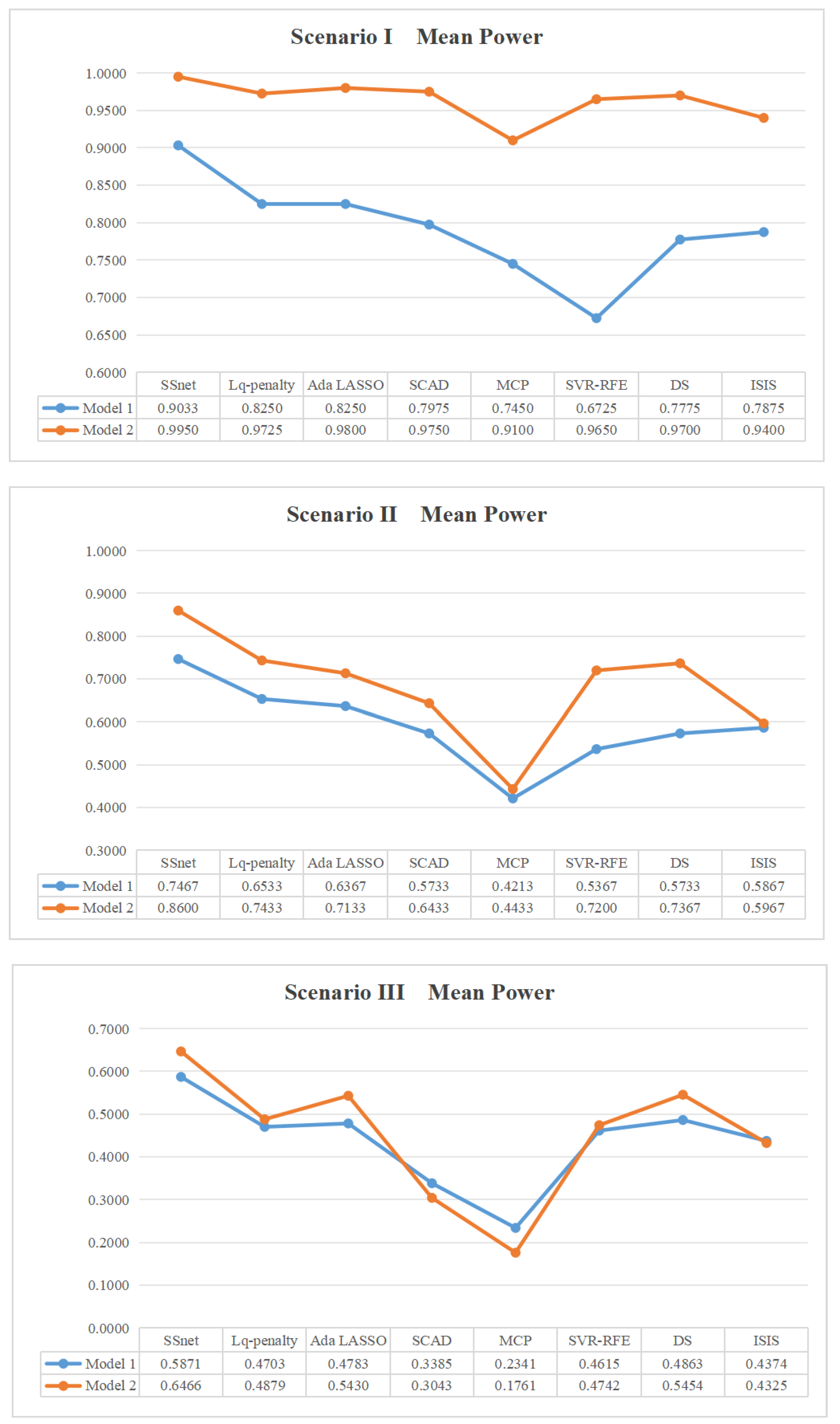
Figure 3.
Mean power in each scenario for SSD .

Table 1.
.
| 1 | 2 | |
|---|---|---|
| 1 | 0 | 0 |
| 2 | 1 | 2 |
| 3 | 2 | 1 |
Table 2.
.
| 1 | 2 | 3 | 4 | |
|---|---|---|---|---|
| 1 | 0 | 0 | 0 | 0 |
| 2 | 1 | 2 | 2 | 1 |
| 3 | 2 | 1 | 1 | 2 |
Table 3.
Williams rubber data.
| 1 | 2 | 3 | 4 | 5 | 6 | 7 | 8 | 9 | 10 | 11 | 12 | 13 | 14 | 15 | 16 | 17 | 18 | 19 | 20 | 21 | 22 | 23 | Response | |
|---|---|---|---|---|---|---|---|---|---|---|---|---|---|---|---|---|---|---|---|---|---|---|---|---|
| 1 | 1 | 1 | 1 | −1 | −1 | −1 | 1 | 1 | 1 | 1 | 1 | −1 | −1 | −1 | 1 | 1 | −1 | −1 | 1 | −1 | −1 | −1 | 1 | 133 |
| 2 | 1 | −1 | −1 | −1 | −1 | −1 | 1 | 1 | 1 | −1 | −1 | −1 | 1 | 1 | 1 | −1 | 1 | −1 | −1 | 1 | 1 | −1 | −1 | 62 |
| 3 | 1 | 1 | −1 | 1 | 1 | −1 | −1 | −1 | −1 | 1 | −1 | 1 | 1 | 1 | 1 | 1 | −1 | −1 | −1 | −1 | 1 | 1 | −1 | 45 |
| 4 | 1 | 1 | −1 | 1 | −1 | 1 | −1 | −1 | −1 | 1 | 1 | −1 | −1 | 1 | 1 | −1 | 1 | 1 | 1 | −1 | −1 | −1 | −1 | 52 |
| 5 | −1 | −1 | 1 | 1 | 1 | 1 | −1 | 1 | 1 | −1 | −1 | −1 | −1 | 1 | 1 | 1 | −1 | −1 | 1 | −1 | 1 | 1 | 1 | 56 |
| 6 | −1 | −1 | 1 | 1 | 1 | 1 | 1 | −1 | 1 | 1 | 1 | −1 | 1 | 1 | −1 | 1 | 1 | 1 | 1 | 1 | 1 | −1 | −1 | 47 |
| 7 | −1 | −1 | −1 | −1 | 1 | −1 | −1 | 1 | −1 | 1 | −1 | 1 | 1 | −1 | 1 | 1 | 1 | 1 | 1 | 1 | −1 | −1 | 1 | 88 |
| 8 | −1 | 1 | 1 | −1 | −1 | 1 | −1 | 1 | −1 | 1 | −1 | −1 | −1 | −1 | −1 | −1 | −1 | 1 | −1 | 1 | 1 | 1 | −1 | 193 |
| 9 | −1 | −1 | −1 | −1 | −1 | 1 | 1 | −1 | −1 | −1 | 1 | 1 | −1 | 1 | −1 | 1 | 1 | −1 | −1 | −1 | −1 | 1 | 1 | 32 |
| 10 | 1 | 1 | 1 | 1 | −1 | 1 | 1 | 1 | −1 | −1 | −1 | 1 | 1 | 1 | −1 | 1 | −1 | 1 | −1 | 1 | −1 | −1 | 1 | 53 |
| 11 | −1 | 1 | −1 | 1 | 1 | −1 | −1 | 1 | 1 | −1 | 1 | −1 | 1 | −1 | −1 | −1 | 1 | 1 | −1 | −1 | −1 | 1 | 1 | 276 |
| 12 | 1 | −1 | −1 | −1 | 1 | 1 | 1 | −1 | 1 | 1 | 1 | 1 | −1 | −1 | 1 | −1 | −1 | 1 | −1 | 1 | 1 | 1 | 1 | 145 |
| 13 | 1 | 1 | 1 | 1 | 1 | −1 | 1 | −1 | 1 | −1 | −1 | 1 | −1 | −1 | −1 | −1 | 1 | −1 | 1 | 1 | −1 | 1 | −1 | 130 |
| 14 | −1 | −1 | 1 | −1 | −1 | −1 | −1 | −1 | −1 | −1 | 1 | 1 | 1 | −1 | −1 | −1 | −1 | −1 | 1 | −1 | 1 | −1 | −1 | 127 |
Table 4.
Results of significant factor screening for each model.
| Variable Selection Method | Size | Significant Factors |
|---|---|---|
| Williams | 4 | 4 10 14 19 |
| SCAD | 8 | 1 4 7 10 11 12 14 19 |
| Ds | 1 | 14 |
| MCP | 3 | 12 14 19 |
| SVR-RFE | 7 | 7 8 9 11 14 15 19 |
| Ada LASSO | 6 | 2 5 8 14 16 22 |
| Lq-penalty | 2 | 14 16 |
| ISIS | 6 | 9 14 15 18 19 20 |
| SSnet | 7 | 4 7 9 12 14 15 19 |
Disclaimer/Publisher’s Note: The statements, opinions and data contained in all publications are solely those of the individual author(s) and contributor(s) and not of MDPI and/or the editor(s). MDPI and/or the editor(s) disclaim responsibility for any injury to people or property resulting from any ideas, methods, instructions or products referred to in the content. |
© 2024 by the authors. Licensee MDPI, Basel, Switzerland. This article is an open access article distributed under the terms and conditions of the Creative Commons Attribution (CC BY) license (https://creativecommons.org/licenses/by/4.0/).
Share and Cite
MDPI and ACS Style
Hong, X.; Zhou, W.; Wang, X.; Li, M. Construction and Analysis for the Optimal Supersaturated Designs with a Large Number of Inert Factors. Axioms 2024, 13, 179. https://doi.org/10.3390/axioms13030179
AMA Style
Hong X, Zhou W, Wang X, Li M. Construction and Analysis for the Optimal Supersaturated Designs with a Large Number of Inert Factors. Axioms. 2024; 13(3):179. https://doi.org/10.3390/axioms13030179
Chicago/Turabian StyleHong, Xiaoqing, Weiping Zhou, Xiao Wang, and Min Li. 2024. "Construction and Analysis for the Optimal Supersaturated Designs with a Large Number of Inert Factors" Axioms 13, no. 3: 179. https://doi.org/10.3390/axioms13030179
Note that from the first issue of 2016, this journal uses article numbers instead of page numbers. See further details here.