

Solutions of Time Fractional (1 + 3)-Dimensional Partial Differential Equations by the Natural Transform Decomposition Method (NTDM)

Mathematics Department, College of Science, King Saud University, P.O. Box 2455, Riyadh 11451, Saudi Arabia
*
Author to whom correspondence should be addressed.
Axioms 2023, 12(10), 958; https://doi.org/10.3390/axioms12100958
Submission received: 12 September 2023
/
Revised: 3 October 2023
/
Accepted: 4 October 2023
/
Published: 11 October 2023
(This article belongs to the Special Issue Special Topics in Differential Equations with Applications)
Abstract
:The current study employs the natural transform decomposition method (NTDM) to test fractional-order partial differential equations (FPDEs). The present technique is a mixture of the natural transform method and the Adomian decomposition method. For the purpose of checking the precis of our technique, some examples are offered, and the series solutions of these equations are introduced by using NTDM. The outcome shows that the suggested approach is very active and straightforward for obtaining a series solutions of FPDEs and is more accurate if we compare it with existing methods.
Keywords:
natural transform; fractional-order linear and nonlinear; approximate solution; inverse natural transformMSC:
35A22; 44A301. Introduction
During the last decades, various numerical methods have been improved in the field of fractional calculus. The fractional differentiation equations play a crucial role in several theoretical physical, biological, and applied engineering problems, such as electromagnetics, viscoelasticity, fluid mechanics, electrochemistry, and biological population models [1,2,3,4,5]. The ADSTM method can be applied to solve the energy balance equations of the porous fin with several temperature dependent properties—see [6]. The authors in [7] discussed the approximate solution of the atmospheric internal waves model by applying FRDTM method. Various approximation and numerical techniques have been utilized to solve fractional differential equations [8,9]. Recently, different new methods for fractional differential equations have been suggested, for example, the fractional differential transform method (FDTM) [10,11], fractional variational iteration method (FVIM) [4], fractional Adomian decomposition method (FROM) [12,13], natural transform decomposition method (NTDM) [14,15,16,17,18], homotopy perturbation method (HPM) [19], and Sumudu transform method (STM) [20,21]. The definition of the natural transform, including its properties, was introduced by Khan in [22], which was later used by Belgacem and his colleagues to obtain the relation between this transform and the Laplace and Sumudu transforms [23]. Some physical problems have been modeled by fractional PDEs and solved by utilizing NTDM, for example, the analytical solution of the system of nonlinear PDEs is proposed in [24]. The main goal of this work is to apply the natural transform decomposition method (NTDM) to solve some types of fractional linear and nonlinear partial differential equations (PDEs). The organization of this work is divided into five sections. In Section 2, definitions and properties of the natural transform method (NTM) are addressed. In Section 3, we discuss the methodology of FNTDM. In Section 4, we offered three examples of fractional PDEs and solved them by NTDM. Finally, Section 5 contains the concluding notions.
2. Basic Definitions and Properties of the Natural Transform Method (NTM)
In this part, some definitions and properties of fractional calculus with natural transform are addressed.
Definition 1.
The natural transform (NT) of a function is defined by the integral [22]
where s and μ are transform variables.
Definition 2.
If where and is natural transform of a function then the (NT) of Caputo fractional derivative of is denoted by [18]
Definition 3.
The inverse natural transform (INTM) of is defined by
Definition 4.
The Caputo operator of order γ for a fractional derivative [25] is presented by the following mathematical expression for :
Definition 5.
Riemann–Liouville fractional order integral [26]:
where describes the concept of the gamma variable by
Important properties: some basic properties of the natural transform method (NTM) are given as follows:
3. Natural Transform and Decomposition Method (NTDM)
Here, we demonstrate the pertinence of the (NTDM) to obtain the general solution of FPDEs.
subject to the initial conditions
where symbols L and N indicate the linear and nonlinear operators, respectively, g is the source function, and is the Caputo operator. By applying the natural transform method (NTM) to both sides of Equation (7), we obtain
By employing the differentiation property of the natural transform method, one can obtain
and
taking the inverse NT for both sides of Equation (11), we obtain
The NTDM solution is described by the following infinite series:
The nonlinear term satisfies the property
Substituting Equations (13) and (14) into Equation (12), we obtain
We define the repetition relation
Therefore, the precise solution is denoted by
4. Illustrative Examples
In this part, we examine the above method using three examples and then compare the approximate solutions with the exact solutions.
Example 1.
Consider the following one-dimensional nonlinear wave-like equation with variable coefficients:
subject to the initial condition
By employing the NTM for both sides of Equation (19), we have
Using the initial conditions in Equation (20) and rearranging the terms, we have
On using the inverse NTM of Equation (22), we have
Now, we assume an infinite series solution for the Equation (23) which is defined by Equation (13); then, Equation (23) becomes
where and are the Adomian polynomials, which represent the nonlinear terms. The few nonlinear terms are as follows:
and
Comparing both sides of Equation (24), we can obtain
The NTDM solution for the above equation is
If we substitute in Equation (27), the approximate solution of Equation (19) becomes
Therefore, the solution of Equation (19) in a closed form is
Figure 1: The solution for Example 1 when .
Figure 2: The solution for Example 1 when .
In the next example, we apply the natural transform decomposition method to solve a non-constant coefficient two-dimensional partial differential equation.
Example 2.
Consider the following two-dimensional fractional wave-like equation [19]:
subject to conditions
Utilizing the NTM for both sides of Equation (29), we can obtain
By placing conditions Equation (30) into Equation (31), we obtain
Employing the inverse natural transform method of Equation (32), we have
Now, we suppose an infinite series solution for the Equation (13); then, Equation (33) becomes
Making both sides of Equation (34) equivalent, we have
The NTDM solution is
If we substitute in Equation (35), the approximate solution of Equation (29) becomes
Hence, the exact solution of Equation (29) in a closed form is
Figure 3: The exact and approximate solutions for Example 2 when .
Figure 4: The exact and approximate solutions for Example 2 when .
Example 3.
Consider the 3D fractional heat equation [19]:
with conditions
Applying the NTM to both sides of Equation (36), we obtain
Taking the inverse NTM of Equation (38), we have
Then, Equation (39) becomes
For
The subsequent terms are given as follows:
The approximate solution of Equation (42) is denoted by
By letting in Equation (43), we have
Therefore, the solution of Equation (36) is provided by
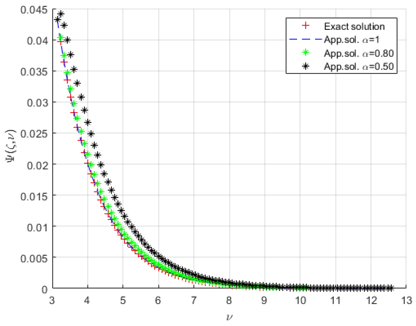
Figure 5: The exact and approximate solutions for Example 3 when .
Figure 6: The exact and approximate solutions for Example 3 when .
In the next example, we apply the natural transform decomposition method to solve the homogeneous time-fractional gas dynamics equation.
Example 4.
Consider the following homogeneous time-fractional gas dynamics equation [27]:
with the initial condition
Taking the NTM of Equation (45) and the initial condition in Equation (46), we have
Taking the inverse NTM of Equation (47), we obtain
Now, we assume an infinite series solution for the Equation (48) given by the form
The nonlinear terms , and are denoted by
where and are Adomian polynomials. Then, Equation (49) becomes
The nonlinear term and are expressed as
and
Making both sides of Equation (51) equivalent, we can obtain
The above equation becomes
take the approximate solution of Equation (55) given by
the solution of Equation (45) is denoted by
Figure 7: The exact and approximate solutions for Example 4 when .
Figure 8: The exact and approximate solutions for Example 4 when .
5. Conclusions
The authors in this work successfully executed the natural transform decomposition method (NTDM) to acquire the approximate solutions of (1+3)-dimensional fractional nonlinear partial differential equations. We have also offered three test problems. The simplicity and high precision of the method show that this technique can be involved in many nonlinear partial differential equations. The NTDM presents a significant improvement in the field over the existing methods such as the optimal homotopy asymptotic method (OHAM) and fractional homotopy analysis transform method (FHATM). In addition to the currently presented methods, it is noteworthy to highlight the discontinuous Galerkin method [28] as a novel and efficient alternative for solving fractional-order linear and nonlinear partial differential equations. Its application to these equations holds substantial potential and can produce promising outcomes. Mathematica software package was applied to obtain the numerical results and graphs.
Author Contributions
Methodology, M.R.G. and H.E.; Writing—original draft, M.R.G.; Writing—review and editing, H.E. All authors have read and agreed to the published version of the manuscript.
Funding
The author would like to extend their sincere appreciation to Researchers Supporting Project number (RSPD 2023R948), King Saud University, Riyadh, Saudi Arabia.
Data Availability Statement
Not applicable.
Conflicts of Interest
The authors declare no conflict of interest.
References
- Caputo, M. Elasticitae Dissipazione; Zanichelli: Bologna, Italy, 1969. [Google Scholar]
- Caputo, M.; Mainardi, F. Linear models of dissipation in anelastic solids. Riv. del Nuovo Cimento. 1971, 1, 161–198. [Google Scholar] [CrossRef]
- Garg, M.; Manohar, P. Numerical solution of fractional diffusion-wave equation with two space variables by matrix method. Fract. Calc. Appl. Anal. 2019, 13, 191–207. [Google Scholar]
- Kilbas, A.A.; Srivastava, H.M.; Trujillo, J.J. Theory and Applications of Fractional Differential Equations; Elsevier: Amsterdam, The Netherlands, 2006. [Google Scholar]
- Rawashdeh, M. An efficient approach for time-fractional damped Burger and time-sharma-tasso-Olver equations using the FRDTM. Appl. Math. Inf. Sci. 2015, 9, 1239–1246. [Google Scholar]
- Patel, T.; Meher, R. Thermal Analysis of porous fin with uniform magnetic field using Adomian decomposition Sumudu transform method. Nonlinear Eng. 2017, 6, 191–200. [Google Scholar] [CrossRef]
- Patel, T.; Patel, H.; Meher, R. Analytical study of atmospheric internal waves model with fractional approach. JOES 2022. [Google Scholar] [CrossRef]
- Omran, M.; Kiliçman, A. Natural transform of fractional order and some properties. Cogent Math. 2016, 3, 1251874. [Google Scholar] [CrossRef]
- Kazem, S. Exact solution of some linear fractional differential equations by Laplace transform. Int. J.Nonlinear Sci. 2013, 16, 3–11. [Google Scholar]
- Odibat, Z.; Momani, S.; Erturk, V.S. Generalized differential transform method: Application to differential equations of fractional order. Appl. Math. Comput. 2008, 197, 467–477. [Google Scholar] [CrossRef]
- Inc, M. The approximate and exact solutions of the space- and time-fractional Burgers equations with initial conditions by variational iteration method. J. Math. Anal. Appl. 2008, 345, 476–484. [Google Scholar] [CrossRef]
- Garg, M.; Sharma, A. Solution of space-time fractional telegraph equation by Adomian decomposition method. J. Inequal. Spec. Funct. 2011, 2, 1–7. [Google Scholar]
- Ray, S.S.; Bera, R.K. An approximate solution of a nonlinear fractional differential equation by Adomian decomposition method. Appl. Math. Comput. 2005, 167, 561–571. [Google Scholar]
- Rawashdeh, M.; Solving, M.S. Nonlinear ordinary differential equations using the NDM. J. Appl. Anal. Comput. 2015, 5, 77–88. [Google Scholar]
- Rawashdeh, M.S.; Al-Jammal, H. New approximate solutions to fractional nonlinear systems of partial differential equations using the FNDM. Adv. Differ. Equ. 2016, 2016, 235. [Google Scholar] [CrossRef]
- Rawashdeh, M.; Maitama, S. Finding exact solutions of nonlinear PDEs using the natural decomposition method. Math. Methods Appl. Sci. 2017, 40, 223–236. [Google Scholar] [CrossRef]
- Cherif, M.H.; Ziane, D.; Belghaba, K. Fractional natural decomposition method for solving fractional system of nonlinear equations of unsteady flow of a polytropic gas. Nonlinear Stud. 2018, 25, 753–764. [Google Scholar]
- Eltayeb, H.; Abdalla, Y.T.; Bachar, I.; Khabir, M.H. Fractional telegraph equation and its solution by natural transform decomposition method. Symmetry 2019, 11, 334. [Google Scholar] [CrossRef]
- Sarwar, S.; Alkhalaf, S.; Iqbal, S.; Zahid, M.A. A note on optimal homotopy asymptotic method for the solutions of fractional order heat- and wave-like partial differential equations. Comput. Math. Appl. 2015, 70, 942–953. [Google Scholar] [CrossRef]
- Katatbeh, Q.D.; Belgacem, F.B.M. Applications of the Sumudu transform to fractional differential equations. Nonlinear Stud. J. 2011, 18, 99–112. [Google Scholar]
- Kumar, D.; Singh, J.; An, K.A. Efficient approach for fractional Harry Dym equation by using Sumudu transform. Abstr. Appl. Anal. 2013, 2013, 608943. [Google Scholar] [CrossRef]
- Khan, Z.H.; Khan, W.A. N-transform properties and applications. NUST J. Eng. Sci. 2008, 1, 127–133. [Google Scholar]
- Belgacem, F.B.M.; Silambarasan, R. Theory of natural transform. Math. Eng. Sci. Aerosp. (MESA) 2012, 3, 99–124. [Google Scholar]
- Marin, M.; Marinescu, C. Thermoelasticity of initially stressed bodies, asymptotic equipartition of energies. Int. J. Eng. Sci. 1998, 36, 73–86. [Google Scholar] [CrossRef]
- Rawashdeh, M.S.; Al-Jammal, H. Theories and Applications of the Inverse Fractional Natural Transform Method. Adv. Differ. 2018, 2018, 222. [Google Scholar] [CrossRef]
- Hilfer, R. Applications of Fractional Calculus in Physics; World Scientific: Singapore, 2000. [Google Scholar]
- Kumar, S.; Rashidi, M. New analytical method for gas dynamics equation arising in shock fronts. Comput. Phys. Commun. 2014, 185, 1947–1954. [Google Scholar] [CrossRef]
- Baccouch, M.; Temimi, H. A high-order space-time ultra-weak discontinuous Galerkin method for the second-order wave equation in one space dimension. J. Comput. Appl. Math. 2021, 389, 113331. [Google Scholar] [CrossRef]
Figure 1.
.
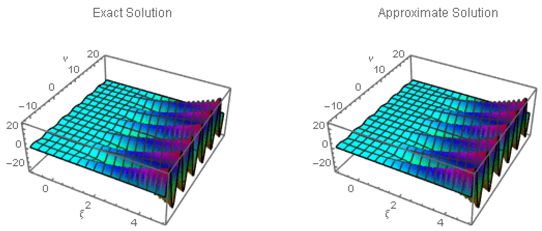
Figure 2.
.
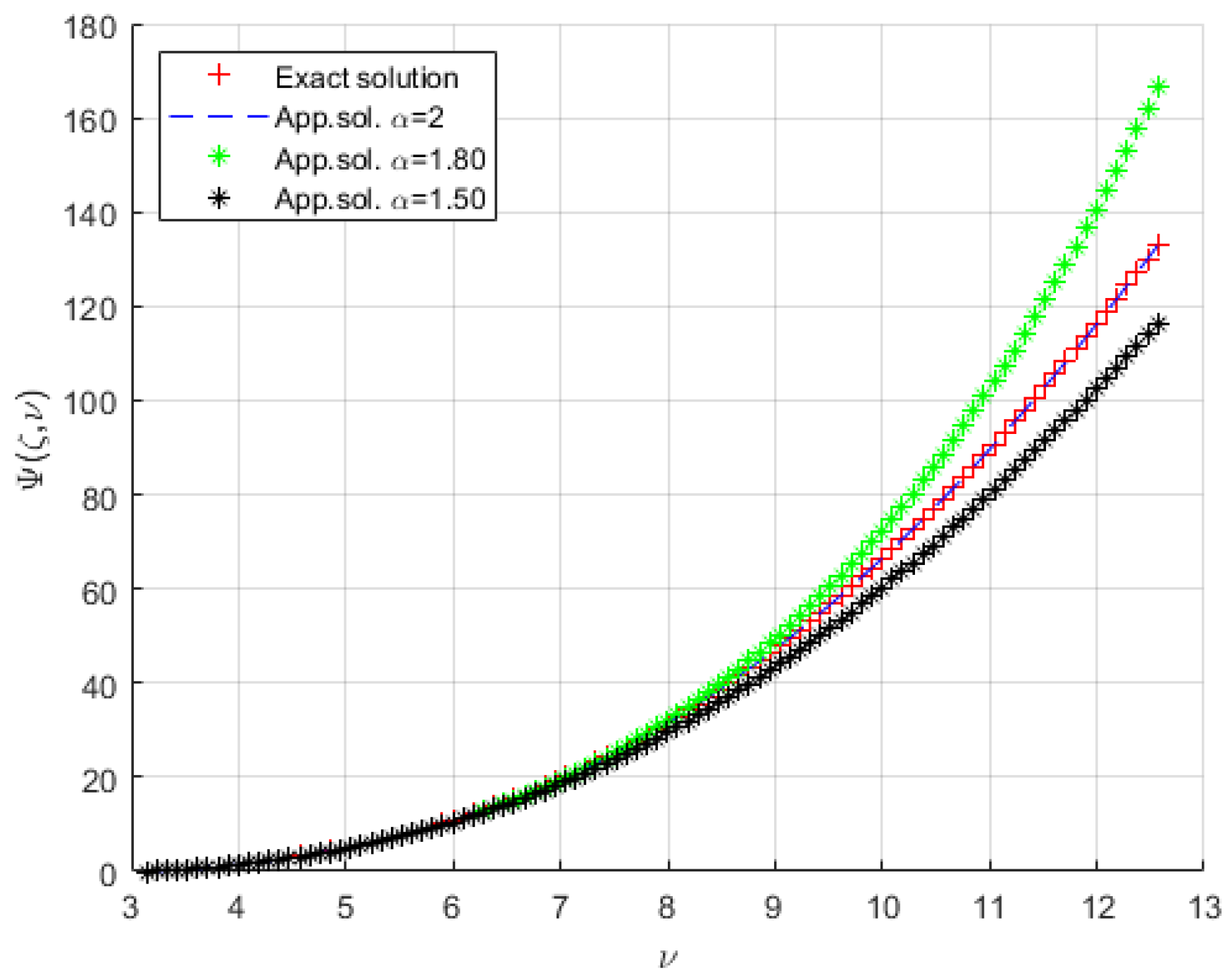
Figure 3.
.
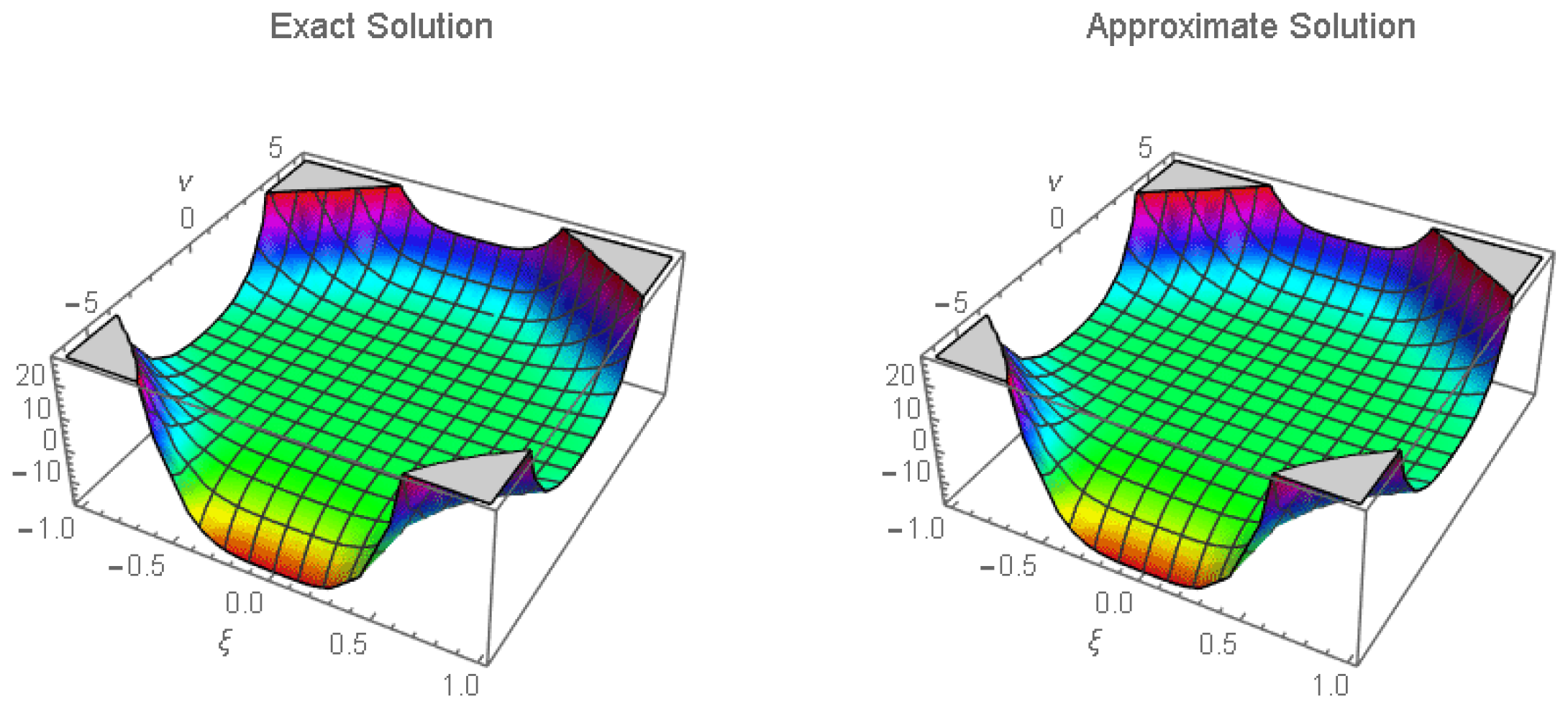
Figure 4.
.

Figure 5.
.

Figure 6.
.

Figure 7.
.
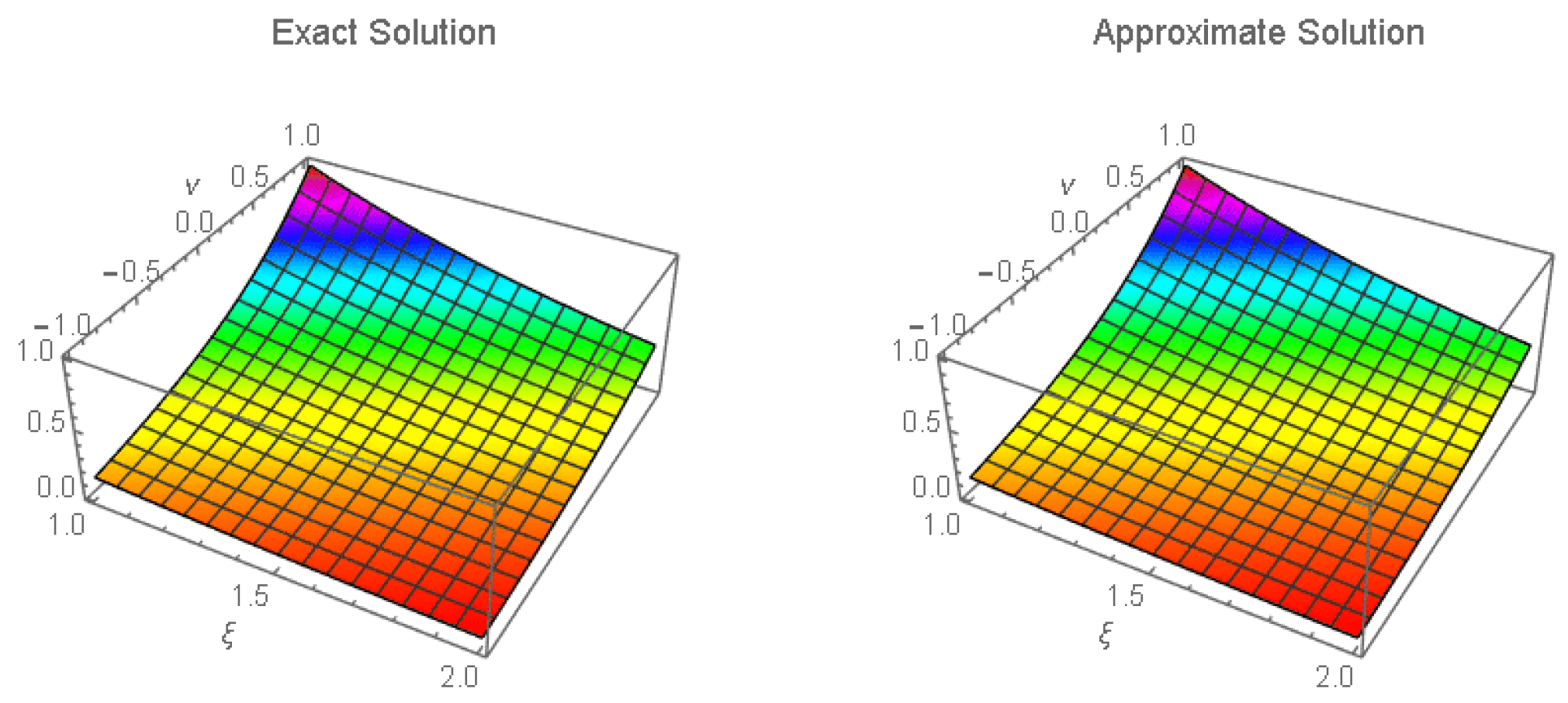
Figure 8.
.

Table 1.
Comparison of the absolute errors for the obtained numerical results and the exact solution for Example 1, for , and
Table 1.
Comparison of the absolute errors for the obtained numerical results and the exact solution for Example 1, for , and
| Exact | Absolute Error | |||||
|---|---|---|---|---|---|---|
| 0.5 | 0.0299640962 | 0.0293796164 | 0.0280835396 | 0.0299640962 | 0 | |
| 0.25 | 0.75 | 0.0513947958 | 0.0452272241 | 0.0384946707 | 0.0426024225 | 0.0087923732 |
| 1 | 0.0734500746 | 0.0501614436 | 0.0460926237 | 0.0010907754 | 0.0723592991 | |
| 0.5 | 0.1302738263 | 0.1175184656 | 0.1123341583 | 01198563846 | 0.0104174417 | |
| 0.50 | 0.75 | 0.2055791830 | 0.1809088961 | 0.153976827 | 0.1704096900 | 0.035169493 |
| 1 | 0.2938002984 | 0.2006457422 | 0.184370449 | 0.0043631016 | 0.2894371968 | |
| 0.5 | 0.5210953055 | 0.4700738629 | 0.4493366329 | 0.4794255386 | 0.0416697669 | |
| 1 | 0.75 | 0.8223167320 | 0.7236355851 | 0.6159147310 | 0.6816387600 | 0.140677972 |
| 1 | 1.175201193 | 0.8025829685 | 0.7374819794 | 0.0174524064 | 1.157748787 |
Table 2.
Comparison of the absolute errors for the obtained numerical results and the exact solution for Example 2, when , and
Table 2.
Comparison of the absolute errors for the obtained numerical results and the exact solution for Example 2, when , and
| Exact | Absolute Error | |||||
|---|---|---|---|---|---|---|
| 0.5 | 0.0064403174 | 0.0066750912 | 0.0072013111 | 0.0064403174 | 1 × 10 | |
| 0.25 | 0.75 | 0.0082695312 | 0.0084681072 | 00096675856 | 0.0082695313 | 6.7 × 10 |
| 1 | 0.0106182872 | 0.0074431273 | 0.0128345819 | 0.0106182883 | 1.19 × 10 | |
| 0.5 | 0.1030451762 | 0.1070299290 | 0.1152209783 | 0.0130450794 | 9.68 × 10 | |
| 0.50 | 0.75 | 0.1323130518 | 0.0885159904 | 0.1546813706 | 0.1323125010 | 5.508 × 10 |
| 1 | 0.1698925954 | 0.1190900375 | 0.2053533103 | 0.1698926143 | 1.89 × 10 | |
| 0.5 | 1.648721270 | 1.708823359 | 1.843435654 | 1.648721270 | 0 | |
| 1 | 0.75 | 2.117000000 | 2.232441653 | 2.474901931 | 2.117000017 | 1.7 × 10 |
| 1 | 2.718281526 | 1.905440600 | 3.285652963 | 2.718281828 | 3.02 × 10 |
Table 3.
Comparison of the absolute errors for the obtained numerical results and the exact solution for Example 3, when .
Table 3.
Comparison of the absolute errors for the obtained numerical results and the exact solution for Example 3, when .
| Exact | Absolute Error | |||||
|---|---|---|---|---|---|---|
| 0.5 | 0.386654 × 10 | 0.481388 × 10 | 0.103833 × 10 | 0.386668 × 10 | 1.39203 × 10 | |
| 0.25 | 0.75 | 0.665619 × 10 | 0.841673 × 10 | 0.157573 × 10 | 0.665783 × 10 | 1.647378 × 10 |
| 1 | 0.102321 × 10 | 0.129654 × 10 | 0.219436 × 10 | 1.024175 × 10 | 9.62711 × 10 | |
| 0.5 | 0.0001583735 | 0.0001971769 | 0.0004253023 | 1.583792 × 10 | 5.7017 × 10 | |
| 0.50 | 0.75 | 0.0002726376 | 0.0003447496 | 0.0006454195 | 2.727050 × 10 | 6.74765 × 10 |
| 1 | 0.0004191080 | 0.0005869575 | 0.0008988117 | 4.195023 × 10 | 3.9432705 × 10 | |
| 0.5 | 0.6486979167 | 0.8076367013 | 1.742038385 | 0.6487212707 | 2.3354 × 10 | |
| 1 | 0.75 | 1.116723633 | 1.412094400 | 2.643638290 | 1.117000017 | 2.76384 × 10 |
| 1 | 1.716666667 | 2.175242941 | 3.681533056 | 1.718281828 | 1.615161 × 10 |
Table 4.
Comparison of the absolute errors for the obtained numerical results and the exact solution for Example 4, with , and
Table 4.
Comparison of the absolute errors for the obtained numerical results and the exact solution for Example 4, with , and
| Exact | Absolute Error | |||||
|---|---|---|---|---|---|---|
| 0.5 | 1.284007229 | 1.501210297 | 2.135501642 | 1.284025417 | 1.8188 × 10 | |
| 0.25 | 0.75 | 1.648506023 | 1.968100996 | 2.837668354 | 1.648721271 | 2.15248 × 10 |
| 1 | 2.115742127 | 2.553826345 | 3.645981610 | 2.117000017 | 1.25789 × 10 | |
| 0.5 | 0.999985352 | 1.169143755 | 1.663130351 | 1 | 1.415448 × 10 | |
| 0.50 | 0.75 | 1.283857782 | 1.532758597 | 2.209978336 | 1.284025417 | 1.67635 × 10 |
| 1 | 1.647741626 | 1.988921957 | 2.839493333 | 1.648721271 | 9.79645 ×10 | |
| 0.5 | 0.6065220684 | 0.7091215329 | 1.008739549 | 0.6065306597 | 8.5913 ×10 | |
| 1 | 0.75 | 0.7786991072 | 0.9296650831 | 1.340419618 | 0.7788007831 | 1.01659 × 10 |
| 1 | 0.9994058152 | 1.206342147 | 1.722239764 | 1 | 5.941848 × 10 |
Disclaimer/Publisher’s Note: The statements, opinions and data contained in all publications are solely those of the individual author(s) and contributor(s) and not of MDPI and/or the editor(s). MDPI and/or the editor(s) disclaim responsibility for any injury to people or property resulting from any ideas, methods, instructions or products referred to in the content. |
© 2023 by the authors. Licensee MDPI, Basel, Switzerland. This article is an open access article distributed under the terms and conditions of the Creative Commons Attribution (CC BY) license (https://creativecommons.org/licenses/by/4.0/).
Share and Cite
MDPI and ACS Style
Gadallah, M.R.; Eltayeb, H. Solutions of Time Fractional (1 + 3)-Dimensional Partial Differential Equations by the Natural Transform Decomposition Method (NTDM). Axioms 2023, 12, 958. https://doi.org/10.3390/axioms12100958
AMA Style
Gadallah MR, Eltayeb H. Solutions of Time Fractional (1 + 3)-Dimensional Partial Differential Equations by the Natural Transform Decomposition Method (NTDM). Axioms. 2023; 12(10):958. https://doi.org/10.3390/axioms12100958
Chicago/Turabian StyleGadallah, Musa Rahamh, and Hassan Eltayeb. 2023. "Solutions of Time Fractional (1 + 3)-Dimensional Partial Differential Equations by the Natural Transform Decomposition Method (NTDM)" Axioms 12, no. 10: 958. https://doi.org/10.3390/axioms12100958
Note that from the first issue of 2016, this journal uses article numbers instead of page numbers. See further details here.