Article

TT-M Finite Element Algorithm for the Coupled Schrödinger–Boussinesq Equations

School of Mathematical Sciences, Inner Mongolia University, Hohhot 010021, China
*
Authors to whom correspondence should be addressed.
These authors contributed equally to this work.
Axioms 2022, 11(7), 314; https://doi.org/10.3390/axioms11070314
Submission received: 5 June 2022 / Revised: 23 June 2022 / Accepted: 24 June 2022 / Published: 28 June 2022
(This article belongs to the Special Issue Numerical Methods for Fractional and Integer PDEs)

Abstract

:
In this article, the coupled Schrödinger–Boussinesq equations are solved numerically using the finite element method combined with the time two-mesh (TT-M) fast algorithm. The spatial direction is discretized by the standard Galerkin finite element method, the temporal direction is approximated by the TT-M Crank–Nicolson scheme, and then the numerical scheme of TT-M finite element (FE) system is formulated. The method includes three main steps: for the first step, the nonlinear system is solved on the coarse time mesh; for the second step, by an interpolation formula, the numerical solutions at the fine time mesh point are computed based on the numerical solutions on the coarse mesh system; for the last step, the linearized temporal fine mesh system is constructed based on Taylor’s formula for two variables, and then the TT-M FE solutions can be obtained. Furthermore, theory analyses on the TT-M system including the stability and error estimations are conducted. Finally, a large number of numerical examples are provided to verify the accuracy of the algorithm, the correctness of theoretical results, and the computational efficiency with a comparison to the numerical results calculated by using the standard FE method.

1. Introduction

The coupled Schrödinger–Boussinesq equations have often been proposed to describe many complex physical processes, such as the dynamic behaviors of the Langmuir soliton formation and the interaction of long-wave with short-wave packets in diatomic lattice systems [1] and nonlinear dispersive media [2,3], where the Schrödinger equation describes the short-wave term and the Boussinesq equation describes the long-wave term. Many theoretical studies have been conducted on this important equation. Guo and Du studied the attractor and its regularity of the damped Schrödinger–Boussinesq equations [4]. The new exact traveling wave solutions of the coupled Schrödinger–Boussinesq equations were constructed, which are expressed by the hyperbolic functions, the trigonometric functions and the rational functions in [5]. Guo studied the existence and uniqueness of global solutions in [6]. Li and Chen proved the existence of global attractors of dissipative Schrödinger–Boussinesq equations [7]. Many other scholars have done a significant amount of work to study the analytical solution of the Schrödinger–Boussinesq equations [8,9,10,11,12,13]. In recent years, many scholars have studied the numerical methods of the Schrödinger–Boussinesq equations. In [3], Liao et al. constructed cubic orthogonal spline collocation schemes to solve Schrödinger–Boussinesq equations, gave conservation laws for schemes, and proved the convergence and stability of the nonlinear scheme by discrete energy methods. In [14], Liao et al. considered the time-splitting Fourier spectral discretization method for solving Schrödinger–Boussinesq equations. In [15], Zhang and Bai developed a conservative difference method for solving Schrödinger–Boussinesq equations, gave the calculation procedure for the numerical solution, and analyzed the related properties. Liao and Zhang [16] developed a conservative compact difference scheme for the N-coupled nonlinear Schrödinger–Boussinesq equations and proved the scheme is unconditionally convergent in the maximum norm. Deng and Wu [17] studied a finite difference method for one-dimensional and two-dimensional nonlinear coupled Schrödinger–Boussinesq equations. In [18], Zheng and Xiang studied the finite element algorithm of coupled Schrödinger–Boussinesq equations and its error theory. Bai and Zhang proposed a quadratic B-spline finite-element method for the coupled Schrödinger–Boussinesq equations and gave an error analysis based on the semi-discrete finite element scheme of the equations in [19]. Other numerical methods to solve the Schrödinger–Boussinesq equations can be found in [20,21,22]. It can be seen from a large number of studies that although there are many numerical methods for solving the coupled Schrödinger–Boussinesq equations, there are few studies on finite element algorithms with fast computing techniques.
In 2018, Liu and his collaborators proposed the fast time two-mesh (TT-M) finite element method in [23] for numerically solving the fractional water wave model. They provided rigorous theory analyses including stability and error estimations, verified the effectiveness of the method by a large number of calculation data, and illustrated the calculation efficiency by making a comparison with the standard nonlinear finite element algorithm. It is easy to find that the TT-M algorithm can save computing time and improve the calculation efficiency to a great extent, and it can be combined with many other algorithms, as summarized in [23]. In view of the advantages of its fast calculation and maintaining calculation accuracy, this method has been developed rapidly. Subsequently, in 2019, Yin et al. developed the TT-M finite element algorithm for a space fractional Allen–Cahn model in [24] and discussed the problem of parameter selection in detail. In [25], Liu et al. used the TT-M finite element method to numerically solve the two-dimensional Gray–Scott model with space fractional derivatives. In [26], Wen et al. used the TT-M algorithm combined with the H 1 -Galerkin mixed finite element method to numerically solve the nonlinear distributed order diffusion model and verified the computational efficiency of the algorithm and the correctness of the theoretical results by numerical examples with smooth and non-smooth solutions. In [27], Wang et al. used the TT-M fast algorithm based on the finite element method to overcome the time-consuming problem caused by the nonlinear term of the strongly nonlinear Allen–Cahn equation. Qiu et al. [28] studied the difference scheme based on the TT-M algorithm to numerically solve the fractional moving/non-moving transport model. Recently, Niu et al. developed a TT-M fourth-order compact difference scheme in [29] and numerically solved the nonlinear distributed fractional Sobolev equation model.
Here, we will develop a TT-M finite element fast algorithm for the initial and boundary value problems of the coupled Schrödinger–Boussinesq equations
i ε E t + γ E x x = λ N E , ( x , t ) ( a , b ) × ( 0 , T ] ,
N t t N x x + α N x x x x θ ( N 2 ) x x = ω ( | E | 2 ) x x , ( x , t ) ( a , b ) × ( 0 , T ] ,
E ( x , 0 ) = E 0 ( x ) , N ( x , 0 ) = N 0 ( x ) , N t ( x , 0 ) = N 1 ( x ) , x [ a , b ] ,
E ( a , t ) = E ( b , t ) = 0 , N ( a , t ) = N ( b , t ) = 0 , t [ 0 , T ] ,
where E is the short-wave amplitude, and N is the long-wave amplitude. E and N are complex functions and real functions, respectively. ε = ( m e / m i ) 1 / 2 , m e and m i are the electronic quality and the ion quality. Parameters α , θ , γ , λ and ω are five positive coefficients. E 0 ( x ) , N 0 ( x ) and N 1 ( x ) are given initial functions.
Now, by introducing the following unknown function Φ ( x , t ) found in many references,
Φ x ( x , t ) = a x N t ( y , t ) d y ,
one can write the original problem (1)–(4) as follows
i ε E t + γ E x x = λ N E , ( x , t ) ( a , b ) × ( 0 , T ] ,
N t = Φ x x , ( x , t ) ( a , b ) × ( 0 , T ] ,
Φ t N + α N x x θ N 2 = ω | E | 2 , ( x , t ) ( a , b ) × ( 0 , T ] ,
E ( x , 0 ) = E 0 ( x ) , N ( x , 0 ) = N 0 ( x ) , Φ ( x , 0 ) = Φ 0 ( x ) , x [ a , b ] ,
E ( a , t ) = E ( b , t ) = 0 , N ( a , t ) = N ( b , t ) = 0 , Φ ( a , t ) = Φ ( b , t ) = 0 , t [ 0 , T ] ,
where Φ ( x , 0 ) = Φ 0 ( x ) is yielded by (5).
In this article, we use the finite element method combined with the TT-M fast algorithm to solve the coupled Schrödinger–Boussinesq equations. The TT-M Crank–Nicolson fast algorithm is used to discretize the time direction and speed up the calculation, and the Galerkin finite element method is used to approximate the space direction. The main work of this article is as follows:
  • Detailed proofs of stability and error estimates for TT-M FE system are done;
  • Numerical examples are given to verify the correctness of the theory results, to reflect the dynamic behavior of solutions and to illustrate the computational efficiency compared with the standard nonliear finite element method.
The remaining structure of this article is as follows: in Section 2, we derive the weak formulation, finite element scheme and the time two-mesh numerical scheme. In Section 3, we give the stability analysis of the TT-M FE system. In Section 4, we derive the optimal error results based on the TT-M system. In Section 5, we carry out the numerical computing by taking some numerical examples. Finally, in Section 6, we provide some discussions for our algorithm and the future studies.
2. Weak Formulation and TT-M Finite Element Scheme

2.1. Weak Formulation

Let Ω ¯ = [ a , b ] . We denote the complex Sobolev space on Ω by the notation H r ( Ω ) = W r , 2 ( Ω ) ,
H 0 1 ( Ω ) = { u H 1 ( Ω ) | u ( a ) = u ( b ) = 0 } .
We denote the inner product in space L 2 ( Ω ) by ( · , · ) , the norm in space L 2 ( Ω ) by · and the norm in space H r ( Ω ) by · r ,
( u , v ) = Ω u v ¯ d x , v = ( v , v ¯ ) 1 / 2 = ( Ω v v ¯ d x ) 1 / 2 ,
v r = v H r = | α | r D α v 2 1 / 2 ,
where v ¯ represents the complex conjugate of v.
Now, the weak formulation for (6)–(10) is to find N, Φ , E H 0 1 ( Ω ) , for g H 0 1 ( Ω ) such that
i ε ( E t , g ) γ ( E x , g x ) = λ ( N E , g ) ,
( N t , g ) = ( Φ x , g x ) ,
( Φ t , g ) ( N , g ) α ( N x , g x ) θ ( N 2 , g ) = ω ( | E | 2 , g ) .
We use the Crank–Nicolson method and rewrite (14)–(16) as follows:
i ε ( E t n + 1 2 , g ) γ ( E x n + 1 2 , g x ) = λ ( N n + 1 2 E n + 1 2 , g ) + ( e 1 ( τ ) n + 1 2 , g ) ,
( N t n + 1 2 , g ) = ( Φ x n + 1 2 , g x ) + ( e 2 ( τ ) n + 1 2 , g ) ,
( Φ t n + 1 2 , g ) ( N n + 1 2 , g ) α ( N x n + 1 2 , g x ) θ ( ( N n + 1 2 ) 2 , g ) = ω ( | E n + 1 2 | 2 , g ) + ( e 3 ( τ ) n + 1 2 , g ) ,
where the truncation errors e 1 ( τ ) n + 1 2 , e 2 ( τ ) n + 1 2 and e 3 ( τ ) n + 1 2 are as follows:
e 1 ( τ ) n + 1 2 = O ( τ 2 ) , e 2 ( τ ) n + 1 2 = O ( τ 2 ) , e 3 ( τ ) n + 1 2 = O ( τ 2 ) .

2.2. TT-M Finite Element Scheme

In order to give the fully discrete scheme of the TT-M FE method, we divide the time interval [ 0 , T ] into a uniform partition with the nodes t n = n M τ ( n = 0 , 1 , , P ) , satisfying 0 = t 0 < t 1 < < t P = T with a positive integer 2 M 1 τ c , where τ = T / ( P M ) and τ c = M τ are the fine time step size and the coarse time step size, respectively. For convenience, we define E t n + 1 2 = E n + 1 E n Δ t and E n + 1 2 = E n + 1 + E n 2 .
The standard nonlinear fully discrete FE scheme corresponding to the weak formulation (17)–(19) is as follows:
i ε ( E h t n + 1 2 , g ) γ ( E h x n + 1 2 , g x ) = λ ( N h n + 1 2 E h n + 1 2 , g ) ,
( N h t n + 1 2 , g ) = ( Φ h x n + 1 2 , g x ) ,
( Φ h t n + 1 2 , g ) ( N h n + 1 2 , g ) α ( N h x n + 1 2 , g x ) θ ( ( N h n + 1 2 ) 2 , g ) = ω ( | E h n + 1 2 | 2 , g ) .
If the numerical calculation is carried out directly through the nonlinear fully discrete FE system (21)–(23), it will take a lot of calculation time. Therefore, we need to develop fast computing methods to improve the computing efficiency. Here, we consider the TT-M fast algorithm based on the FE method, which includes three main calculating steps (see [23]):
Step 1: The coarse time mesh system based on the coarse time step τ c is solved directly by the iterative algorithm.
i ε ( E c t n + 1 2 , g ) γ ( E c x n + 1 2 , g x ) = λ ( N c n + 1 2 E c n + 1 2 , g ) ,
( N c t n + 1 2 , g ) = ( Φ c x n + 1 2 , g x ) ,
( Φ c t n + 1 2 , g ) ( N c n + 1 2 , g ) α ( N c x n + 1 2 , g x ) θ ( ( N c n + 1 2 ) 2 , g ) = ω ( | E c n + 1 2 | 2 , g ) .
Step 2: Now, we need to expand the nodes and the corresponding point values. We let m be the index of the fine time mesh, m = 0 , 1 , , M 1 , M , , M P . Taking n = m M to be the smallest integer that is equal to or greater than m M , we use an interpolation formula and obtain
E I m = λ m E c n 1 + ( 1 λ m ) E c n ,
where λ m = n m M [ 0 , 1 ) . We obtain all the interpolated values E I m ( E I 0 = E c 0 ) at time t m ( m = 1 , , M 1 , M , , P M ) between E c n 1 and E c n ( n = 1 , 2 , , P ) . Similarly, we can define N I m as
N I m = λ m N c n 1 + ( 1 λ m ) N c n .
Step 3: Based on all the coarse numerical solutions obtained in Step 2, Taylor’s formula for two variables is performed to obtain a linearized system on a fine time step τ ,
i ε ( E f t m + 1 2 , g ) γ ( E f x m + 1 2 , g x ) = λ ( f ( N I m + 1 2 , E I m + 1 2 ) + f N I ( N I m + 1 2 , E I m + 1 2 ) ( N f m + 1 2 N I m + 1 2 ) + f E I ( N I m + 1 2 , E I m + 1 2 ) ( E f m + 1 2 E I m + 1 2 ) , g ) ,
( N f t m + 1 2 , g ) = ( Φ f x m + 1 2 , g x ) ,
( Φ f t m + 1 2 , g ) ( N f m + 1 2 , g ) α ( N f x m + 1 2 , g x ) = θ ( y ( N I m + 1 2 ) + y N I ( N I m + 1 2 ) ( N f m + 1 2 N I m + 1 2 ) , g ) + ω ( q ( E I m + 1 2 ) + q E I ( E I m + 1 2 ) ( E f m + 1 2 E I m + 1 2 ) , g ) ,
where
f ( N f m + 1 2 , E f m + 1 2 ) = N f m + 1 2 E f m + 1 2 , y ( N f m + 1 2 ) = ( N f m + 1 2 ) 2 , q ( E f m + 1 2 ) = | E f m + 1 2 | 2 .
The TT-M numerical solutions are obtained by directly solving (29)–(31).
We will discuss the stability and error estimation of the TT-M FE system. Without losing generality, in the following analysis process, we take the coefficient parameter in the model (1) as ε = α = θ = 1 , γ = 3 2 , λ = 1 2 and ω = 1 4 .
Remark 1.
Compared with semi-implicit and semi-explicit schemes [17,30,31], the purpose of the TT-M FE algorithm is to solve the nonlinear system directly. Moreover, with a comparison to the standard nonlinear Galerkin FE method, our algorithm can save on computing time, which can be seen by observing the numerical results.

3. Stability Analysis

In this section, we give the stability analysis of the TT-M FE scheme.
Theorem 1.
The following stability for the fully discrete scheme (24)(26) on the coarse time mesh holds:
E c n 2 + Φ c n 2 + N c n 2 C ( E c 0 2 + Φ c 0 2 + N c 0 2 ) .
Proof. 
Choosing g = E c n + 1 2 in (24) and taking the imaginary part and setting g = N c n + 1 2 in (25) and g = Φ c n + 1 2 in (26), we combine the three resulting equations to arrive at
1 2 τ ( E c n + 1 2 E c n 2 + Φ c n + 1 2 Φ c n 2 + N c n + 1 2 N c n 2 ) ( N c n + 1 + N c n 2 , Φ c n + 1 + Φ c n 2 ) = ( ( N c n + 1 2 ) 2 , Φ c n + 1 + Φ c n 2 ) + 1 4 ( | E c n + 1 2 | 2 , Φ c n + 1 + Φ c n 2 ) .
Summing (33) from 0 to n and using the Hölder inequality and Young inequality, we have
1 2 τ ( E c n + 1 2 E c 0 2 + Φ c n + 1 2 Φ c 0 2 + N c n + 1 2 N c 0 2 ) k = 0 n ( N c k + 1 2 N c k + 1 2 + 1 4 E c k + 1 2 E c k + 1 2 ) Φ c k + 1 + Φ c k 2 + C k = 0 n ( N c k + 1 2 2 + Φ c k + 1 2 2 ) .
Using the Gronwall inequality with a small enough τ , we obtain
E c n + 1 2 + Φ c n + 1 2 + N c n + 1 2 C ( E c 0 2 + Φ c 0 2 + N c 0 2 ) .
Remark 2.
Actually, we easily obtain the following two conservation relationships by referring to [18]:
E c n = E c 0 , N c n = N c 0 .
Theorem 2.
The stability holds for the TT-M FE system (29)(31)
E f m + 1 2 + Φ f m + 1 2 + N f m + 1 2 C ( E f 0 2 + Φ f 0 2 + N f 0 2 + E c 0 2 + Φ c 0 2 + N c 0 2 ) .
Proof. 
Setting g = E f m + 1 2 in (29) and taking the imaginary part, and using the Hölder inequality as well as the Young inequality, we have
1 2 τ ( E f m + 1 2 E f m 2 ) = I m ( N f m + 1 2 E I m + 1 2 + N I m + 1 2 E f m + 1 2 N I m + 1 2 E I m + 1 2 , E f m + 1 2 ) C ( N I m + 1 2 2 + E I m + 1 2 2 + N f m + 1 2 2 + E f m + 1 2 2 ) .
Summing (38) from 0 to m 1 , we get
E f m 2 E f 0 2 C τ k = 0 m 1 ( N I k 2 + E I k 2 + N f k 2 + E f k 2 ) .
Using (27) and (28), the triangle inequality and Theorem 1, we have
E I m = λ m E c n 1 + ( 1 λ m ) E c n λ m E c n 1 + ( 1 λ m ) E c n C ( E c 0 2 + Φ c 0 2 + N c 0 2 ) ,
and
N I m = λ m N c n 1 + ( 1 λ m ) N c n λ m N c n 1 + ( 1 λ m ) N c n C ( E c 0 2 + Φ c 0 2 + N c 0 2 ) .
Combining (39)–(41) with the Gronwall inequality, we arrive at
E f m 2 C ( N c 0 2 + E c 0 2 + Φ c 0 2 + N f 0 2 + E f 0 2 ) .
Setting g = N f m + 1 2 in (30) and g = Φ f m + 1 2 in (31) and combining two resulting equations, we arrive at
( Φ f m + 1 Φ f m τ , Φ f m + 1 + Φ f m 2 ) + ( N f m + 1 N f m τ , N f m + 1 + N f m 2 ) ( N f m + 1 + N f m 2 , Φ f m + 1 + Φ f m 2 ) = ( ( N I m + 1 2 ) 2 + 2 N I m + 1 2 ( N f m + 1 2 N I m + 1 2 ) , Φ f m + 1 + Φ f m 2 ) + 1 4 ( | E I m + 1 2 | 2 + 2 | E I m + 1 2 | ( E f m + 1 2 E I m + 1 2 ) , Φ f m + 1 + Φ f m 2 ) .
Summing (43) from 0 to m 1 and using the Hölder inequality as well as the Young inequality, we have
1 2 τ ( Φ f m + 1 2 Φ f 0 2 ) + 1 2 τ ( N f m + 1 2 N f 0 2 ) k = 0 m 1 ( N I k + 1 2 N I k + 1 2 + 2 N I k + 1 2 N f k + 1 2 N I k + 1 2 + 1 4 E I k + 1 2 E I k + 1 2 + 1 2 E I k + 1 2 E f k + 1 2 E I k + 1 2 ) Φ f k + 1 + Φ f k 2 + C k = 0 m 1 ( N f k + 1 2 2 + Φ f k + 1 2 2 ) .
Combining (44) with (42) and using the Young inequality, we have
E f m + 1 2 + Φ f m + 1 2 + N f m + 1 2 C ( N c 0 2 + E c 0 2 + Φ c 0 2 + N f 0 2 + E f 0 2 + Φ f 0 2 ) + C τ k = 0 m N I k + 1 2 2 N I k + 1 2 2 + C τ k = 0 m N I k + 1 2 2 N f k + 1 2 N I k + 1 2 2 + C τ k = 0 m E I k + 1 2 2 E I k + 1 2 2 + C τ k = 0 m E I k + 1 2 2 E f k + 1 2 E I k + 1 2 2 + C ε τ k = 0 m ( N f k + 1 2 2 + Φ f k + 1 2 2 ) C ( N c 0 2 + E c 0 2 + Φ c 0 2 + N f 0 2 + E f 0 2 + Φ f 0 2 ) + C τ k = 0 m ( N I k + 1 2 2 + E I k + 1 2 2 + N f k + 1 2 2 + E f k + 1 2 2 + Φ f k + 1 2 2 ) .
Using the Gronwall inequality with a small enough τ , we obtain the conclusion of theorem. □

4. Error Analysis

In this section, we will present an error analysis on the TT-M FE scheme. We introduce the auxiliary projection Q h on S h ( Ω ) defined by: for v H 0 1 ( Ω ) ,
( ( Q h v v ) x , w h x ) = 0 , w h S h ,
where Q h satisfies the following inequalities.
Lemma 1
(See [32]). Assuming that a function v satisfies the condition
v H 0 1 ( Ω ) H r + 1 ( Ω ) ,
then the following inequalities hold:
Q h v v + ( Q h v v ) t + h Q h v v 1 C h r + 1 ( v r + 1 + v t r + 1 ) ,
where C is the constant independent of h.
Theorem 3.
Let E n , N n , Φ n be the solution of system (6)(8), and suppose E c n , N c n , Φ c n and E f m , N f m , Φ f m are the solutions ofthe FE system (24)(26) and the TT-M FE system (29)(31), respectively. Then, there exists a constant C > 0 that depends only on E n , N n , Φ n , such that
E c n E n + N c n N n + Φ c n Φ n C ( τ c 2 + h r + 1 ) ,
and
E f m E m + N f m N m + Φ f m Φ m C ( τ c 4 + τ 2 + h r + 1 ) .
Proof. 
Here, we will prove the theorem by two main steps: (i) estimates on the coarse time mesh; (ii) estimates on the fine time mesh.
(i) Firstly, we derive error results based on the coarse time mesh. To facilitate the derivation, we split the errors as the following:
E c n + 1 2 E n + 1 2 = E c n + 1 2 Q h E n + 1 2 + Q h E n + 1 2 E n + 1 2 = μ 1 n + 1 2 + σ 1 n + 1 2 ,
N c n + 1 2 N n + 1 2 = N c n + 1 2 Q h N n + 1 2 + Q h N n + 1 2 N n + 1 2 = μ 2 n + 1 2 + σ 2 n + 1 2 ,
Φ c n + 1 2 Φ n + 1 2 = Φ c n + 1 2 Q h Φ n + 1 2 + Q h Φ n + 1 2 Φ n + 1 2 = μ 3 n + 1 2 + σ 3 n + 1 2 .
Combining (17)–(19) with (24)–(26), we easily write the error equations as
i ( μ 1 t n + 1 2 , g ) + i ( σ 1 t n + 1 2 , g ) 3 2 ( μ 1 x n + 1 2 , g x ) = 1 2 ( N c n + 1 2 E c n + 1 2 N n + 1 2 E n + 1 2 , g ) + ( e 1 ( τ c ) n + 1 2 , g ) ,
( μ 2 t n + 1 2 , g ) + ( σ 2 t n + 1 2 , g ) = ( μ 3 x n + 1 2 , g x ) + ( e 2 ( τ c ) n + 1 2 , g ) ,
( μ 3 t n + 1 2 , g ) + ( σ 3 t n + 1 2 , g ) ( μ 2 n + 1 2 , g ) ( σ 2 n + 1 2 , g ) ( μ 2 x n + 1 2 , g x ) = ( ( N c n + 1 2 ) 2 ( N n + 1 2 ) 2 , g ) + 1 4 ( | E c n + 1 2 | 2 | E n + 1 2 | 2 , g ) + ( e 3 ( τ c ) n + 1 2 , g ) .
Choosing g = μ 1 n + 1 2 in (50) and taking the imaginary part of the resulting equation, using the Hölder inequality and the boundedness of E c , N c , E and N , we get
μ 1 n + 1 2 μ 1 n 2 = 2 τ R e ( σ 1 n + 1 σ 1 n τ , μ 1 n + 1 2 ) + τ I m ( N c n + 1 2 E c n + 1 2 N n + 1 2 E n + 1 2 , μ 1 n + 1 2 ) + 2 τ I m ( e 1 ( τ c ) n + 1 2 , μ 1 n + 1 2 ) 2 τ ( σ 1 n + 1 σ 1 n τ 2 + μ 1 n + 1 2 + μ 1 n 2 ) + C τ ( μ 1 n + 1 2 + μ 1 n 2 + σ 1 n + 1 2 + σ 1 n 2 + μ 2 n + 1 2 + μ 2 n 2 + σ 2 n + 1 2 + σ 2 n 2 + e 1 ( τ c ) n + 1 2 + e 1 ( τ c ) n 2 ) .
Setting g = μ 2 n + 1 2 in (51) and taking g = μ 3 n + 1 2 in (52), by the similar derivation to [18], we easily have
μ 1 n + 1 2 μ 1 n 2 + μ 2 n + 1 2 μ 2 n 2 + μ 3 n + 1 2 μ 3 n 2 C τ ( μ 1 n + 1 2 + μ 1 n 2 + μ 2 n + 1 2 + μ 2 n 2 + μ 3 n + 1 2 + μ 3 n 2 + σ 1 n + 1 2 + σ 1 n 2 + σ 2 n + 1 2 + σ 2 n 2 + σ 1 n + 1 σ 1 n τ 2 + σ 2 n + 1 σ 2 n τ 2 + σ 3 n + 1 σ 3 n τ 2 + e 1 ( τ c ) n + 1 2 + e 1 ( τ c ) n 2 + e 2 ( τ c ) n + 1 2 + e 2 ( τ c ) n 2 + e 3 ( τ c ) n + 1 2 + e 3 ( τ c ) n 2 ) .
Summing (54) from 0 to n and using the Gronwall inequality, Lemma 1 and the triangle inequality, we have
E c n + 1 E n + 1 + N c n + 1 N n + 1 + Φ c n + 1 Φ n + 1 C ( τ c 2 + h r + 1 ) .
Taking the similar techniques to (40) and (41), we easily obtain
E I m + 1 E m + 1 + N I m + 1 N m + 1 + Φ I m + 1 Φ m + 1 C ( τ c 2 + h r + 1 ) ,
which will be used in the following analysis.
(ii) Secondly, we give a detailed analysis on the fine time mesh. We rewrite the errors as
E f m + 1 2 E m + 1 2 = E f m + 1 2 Q h E m + 1 2 + Q h E m + 1 2 E m + 1 2 = ξ 1 m + 1 2 + ρ 1 m + 1 2 ,
N f m + 1 2 N m + 1 2 = N f m + 1 2 Q h N m + 1 2 + Q h N m + 1 2 N m + 1 2 = ξ 2 m + 1 2 + ρ 2 m + 1 2 ,
Φ f m + 1 2 Φ m + 1 2 = Φ f m + 1 2 Q h Φ m + 1 2 + Q h Φ m + 1 2 Φ m + 1 2 = ξ 3 m + 1 2 + ρ 3 m + 1 2 .
Combining (17)–(19) with (29)–(31), we can obtain the following error equations:
i ( ξ 1 t m + 1 2 , g ) + i ( ρ 1 t m + 1 2 , g ) 3 2 ( ξ 1 x m + 1 2 , g x ) = 1 2 ( f ( N I m + 1 2 , E I m + 1 2 ) + f N I ( N I m + 1 2 , E I m + 1 2 ) ( N f m + 1 2 N I m + 1 2 ) + f E I ( N I m + 1 2 , E I m + 1 2 ) ( E f m + 1 2 E I m + 1 2 ) f ( N m + 1 2 , E m + 1 2 ) , g ) + ( e 1 ( τ ) m + 1 2 , g ) ,
( ξ 2 t m + 1 2 , g ) + ( ρ 2 t m + 1 2 , g ) = ( ξ 3 x m + 1 2 , g x ) + ( e 2 ( τ ) m + 1 2 , g ) ,
and
( ξ 3 t m + 1 2 , g ) + ( ρ 3 t m + 1 2 , g ) ( ξ 2 m + 1 2 , g ) ( ρ 2 m + 1 2 , g ) ( ξ 2 x m + 1 2 , g x ) = ( y ( N I m + 1 2 ) + y N I ( N I m + 1 2 ) ( N f m + 1 2 N I m + 1 2 ) y ( N m + 1 2 ) , g ) + 1 4 ( q ( E I m + 1 2 ) + q E I ( E I m + 1 2 ) ( E f m + 1 2 E I m + 1 2 ) q ( E m + 1 2 ) , g ) + ( e 3 ( τ ) m + 1 2 , g ) .
By Taylor’s formula for two variables, we can derive
f ( N I m + 1 2 , E I m + 1 2 ) + f N I ( N I m + 1 2 , E I m + 1 2 ) ( N f m + 1 2 N I m + 1 2 ) + f E I ( N I m + 1 2 , E I m + 1 2 ) ( E f m + 1 2 E I m + 1 2 ) f ( N m + 1 2 , E m + 1 2 ) = f N I ( N I m + 1 2 , E I m + 1 2 ) ( ξ 2 m + 1 2 + ρ 2 m + 1 2 ) + f E I ( N I m + 1 2 , E I m + 1 2 ) ( ξ 1 m + 1 2 + ρ 1 m + 1 2 ) 1 2 { f N I N I ( N I m + 1 2 , E I m + 1 2 ) ( N m + 1 2 N I m + 1 2 ) 2 + f E I E I ( N I m + 1 2 , E I m + 1 2 ) ( E m + 1 2 E I m + 1 2 ) 2 + 2 f N I E I ( N I m + 1 2 , E I m + 1 2 ) ( N m + 1 2 N I m + 1 2 ) ( E m + 1 2 E I m + 1 2 ) } = N I m + 1 2 ( ξ 1 n + 1 2 + ρ 1 n + 1 2 ) + E I m + 1 2 ( ξ 2 n + 1 2 + ρ 2 n + 1 2 ) ( N m + 1 2 N I m + 1 2 ) ( E m + 1 2 E I m + 1 2 ) .
In (57), we set g = ξ 1 m + 1 2 and take the imaginary part to get
ξ 1 m + 1 2 ξ 1 m 2 = 2 τ R e ρ 1 m + 1 ρ 1 m τ , ξ 1 m + 1 2 + τ I m ( f ( N I m + 1 2 , E I m + 1 2 ) + f N I ( N I m + 1 2 , E I m + 1 2 ) ( N f m + 1 2 N I m + 1 2 ) + f E I ( N I m + 1 2 , E I m + 1 2 ) ( E f m + 1 2 E I m + 1 2 ) f ( N m + 1 2 , E m + 1 2 ) , ξ 1 m + 1 2 ) + 2 τ I m ( e 1 ( τ ) m + 1 2 , ξ 1 m + 1 2 ) 2 τ ρ 1 m + 1 ρ 1 m τ 2 + ξ 1 m + 1 2 + ξ 1 m 2 + C τ ( ξ 1 m + 1 2 + ξ 1 m 2 + ρ 1 m + 1 2 + ρ 1 m 2 + ξ 2 m + 1 2 + ξ 2 m 2 + ρ 2 m + 1 2 + ρ 2 m 2 + ( N m + 1 2 N I m + 1 2 ) ( E m + 1 2 E I m + 1 2 ) 2 + e 1 ( τ ) m + 1 2 + e 1 ( τ ) m 2 ) .
Setting g = ξ 2 m + 1 2 in (58), we get
1 2 τ a b ( ( ξ 2 m + 1 ) 2 ( ξ 2 m ) 2 ) d x + 1 2 a b ρ 2 m + 1 ρ 2 m τ ( ξ 2 m + 1 + ξ 2 m ) d x = 1 4 a b ( ξ 3 x m + 1 + ξ 3 x m ) ( ξ 2 x m + 1 + ξ 2 x m ) d x + 1 4 a b ( e 2 ( τ ) m + 1 + e 2 ( τ ) m ) ( ξ 2 m + 1 + ξ 2 m ) d x .
Take g = ξ 3 m + 1 2 in (59), we arrive at
1 2 τ a b ( ( ξ 3 m + 1 ) 2 ( ξ 3 m ) 2 ) d x + 1 2 a b ρ 3 m + 1 ρ 3 m τ ( ξ 3 m + 1 + ξ 3 m ) d x 1 4 a b ( ξ 2 m + 1 + ξ 2 m ) ( ξ 3 m + 1 + ξ 3 m ) d x 1 4 a b ( ρ 2 m + 1 + ρ 2 m ) ( ξ 3 m + 1 + ξ 3 m ) d x 1 4 a b ( ξ 2 x m + 1 + ξ 2 x m ) ( ξ 3 x m + 1 + ξ 3 x m ) d x = 1 8 a b [ ( 2 | E I m + 1 2 | ( ξ 1 m + 1 2 + ρ 1 m + 1 2 ) + ( E m + 1 2 E I m + 1 2 ) 2 ] ( ξ 3 m + 1 + ξ 3 m ) d x + 1 2 a b [ ( 2 N I m + 1 2 ( ξ 2 m + 1 2 + ρ 2 m + 1 2 ) + ( N m + 1 2 N I m + 1 2 ) 2 ] ( ξ 3 m + 1 + ξ 3 m ) d x + 1 4 a b ( e 3 ( τ ) m + 1 + e 3 ( τ ) m ) ( ξ 3 m + 1 + ξ 3 m ) d x .
Combining (62) with (63), we obtain
1 2 τ a b ( ( ξ 2 m + 1 ) 2 ( ξ 2 m ) 2 + ( ξ 3 m + 1 ) 2 ( ξ 3 m ) 2 ) d x = R 3 + R 4 ,
where R 3 and R 4 are given as follows:
R 3 = 1 2 a b ρ 2 m + 1 ρ 2 m τ ( ξ 2 m + 1 + ξ 2 m ) d x 1 4 a b ( ξ 3 x m + 1 + ξ 3 x m ) ( ξ 2 x m + 1 + ξ 2 x m ) d x + 1 4 a b ( e 2 ( τ ) m + 1 + e 2 ( τ ) m ) ( ξ 2 m + 1 + ξ 2 m ) d x ,
R 4 = 1 2 a b ρ 3 m + 1 ρ 3 m τ ( ξ 3 m + 1 + ξ 3 m ) d x + 1 4 a b ( ξ 2 m + 1 + ξ 2 m ) ( ξ 3 m + 1 + ξ 3 m ) d x + 1 4 a b ( ρ 2 m + 1 + ρ 2 m ) ( ξ 3 m + 1 + ξ 3 m ) d x + 1 4 a b ( ξ 2 x m + 1 + ξ 2 x m ) ( ξ 3 x m + 1 + ξ 3 x m ) d x + 1 8 a b [ ( 2 | E I m + 1 2 | ( ξ 1 m + 1 2 + ρ 1 m + 1 2 ) + ( E m + 1 2 E I m + 1 2 ) 2 ] ( ξ 3 m + 1 + ξ 3 m ) d x + 1 2 a b [ ( 2 N I m + 1 2 ( ξ 2 m + 1 2 + ρ 2 m + 1 2 ) + ( N m + 1 2 N I m + 1 2 ) 2 ] ( ξ 3 m + 1 + ξ 3 m ) d x + 1 4 a b ( e 3 ( τ ) m + 1 + e 3 ( τ ) m ) ( ξ 3 m + 1 + ξ 3 m ) d x .
Adding (65) and (66) together, and using the Cauchy–Schwarz inequality as well as the Young inequality, we get
R 3 + R 4 1 2 a b ρ 2 m + 1 ρ 2 m τ 2 + ( ξ 2 m + 1 ) 2 + ( ξ 2 m ) 2 d x + C a b [ ( ξ 2 m + 1 ) 2 + ( ξ 2 m ) 2 + ( e 2 ( τ ) m + 1 ) 2 + ( e 2 ( τ ) m ) 2 ] d x + 1 2 a b ρ 3 m + 1 ρ 3 m τ 2 + ( ξ 3 m + 1 ) 2 + ( ξ 3 m ) 2 d x + C a b [ ( ξ 3 m + 1 ) 2 + ( ξ 3 m ) 2 + ( ξ 2 m + 1 ) 2 + ( ξ 2 m ) 2 + ( ξ 1 m + 1 ) 2 + ( ξ 1 m ) 2 + ( ρ 1 m + 1 ) 2 + ( ρ 1 m ) 2 + ( ρ 2 m + 1 ) 2 + ( ρ 2 m ) 2 + ( ( E m + 1 2 E I m + 1 2 ) 2 ) 2 + ( ( N m + 1 2 N I m + 1 2 ) 2 ) 2 + ( e 3 ( τ ) m + 1 ) 2 + ( e 3 ( τ ) m ) 2 ] d x .
Combining (61) with (67), we have
ξ 1 m + 1 2 ξ 1 m 2 + ξ 2 m + 1 2 ξ 2 m 2 + ξ 3 m + 1 2 ξ 3 m 2 C τ ( ξ 1 m + 1 2 + ξ 1 m 2 + ξ 2 m + 1 2 + ξ 2 m 2 + ξ 3 m + 1 2 + ξ 3 m 2 + ρ 1 m + 1 2 + ρ 1 m 2 + ρ 2 m + 1 2 + ρ 2 m 2 + ρ 1 m + 1 ρ 1 m τ 2 + ρ 2 m + 1 ρ 2 m τ 2 + ρ 3 m + 1 ρ 3 m τ 2 + ( E m + 1 2 E I m + 1 2 ) 2 2 + ( N m + 1 2 N I m + 1 2 ) 2 2 + ( N m + 1 2 N I m + 1 2 ) ( E m + 1 2 E I m + 1 2 ) 2 + e 1 ( τ ) m + 1 2 + e 1 ( τ ) m 2 + e 2 ( τ ) m + 1 2 + e 2 ( τ ) m 2 + e 3 ( τ ) m + 1 2 + e 3 ( τ ) m 2 ) .
Making use of (56), the Hölder inequality and the similar technique as shown in [33], we have
( E m + 1 2 E I m + 1 2 ) 2 2 + ( N m + 1 2 N I m + 1 2 ) 2 2 + ( N m + 1 2 N I m + 1 2 ) ( E m + 1 2 E I m + 1 2 ) 2 E m + 1 2 E I m + 1 2 2 E m + 1 2 E I m + 1 2 2 + N m + 1 2 N I m + 1 2 2 ( N m + 1 2 N I m + 1 2 2 + E m + 1 2 E I m + 1 2 2 ) C ( τ c 4 + h 2 r + 2 ) .
Combining (68) with (69), and summing the resulting equation from 0 to m, we arrive at
ξ 1 m + 1 2 + ξ 2 m + 1 2 + ξ 3 m + 1 2 ξ 1 0 2 + ξ 2 0 2 + ξ 3 0 2 + C τ k = 0 m ( ξ 1 k + 1 2 + ξ 2 k + 1 2 + ξ 3 k + 1 2 + ρ 1 k + 1 2 + ρ 2 k + 1 2 + ρ 1 k + 1 ρ 1 k τ 2 + ρ 2 k + 1 ρ 2 k τ 2 + ρ 3 k + 1 ρ 3 k τ 2 + τ c 4 + h 2 r + 2 + e 1 ( τ ) k + 1 2 + e 2 ( τ ) k + 1 2 + e 3 ( τ ) k + 1 2 ) .
Using the Gronwall inequality and Lemma 1, we finish the proof of the theorem. □

5. Numerical Tests

We denote Ξ Q η n ( τ , h ) max n Q n Q η n , where η = h or f and define the convergence rate by the following formula:
Rate = log 2 [ Ξ Q η n ( 2 τ , h ) / Ξ Q η n ( τ , h ) ] , in   time , log 2 [ Ξ Q η n ( τ , 2 h ) / Ξ Q η n ( τ , h ) ] , in   space , log 2 [ Ξ Q η n ( 2 τ , 2 h ) / Ξ Q η n ( τ , h ) ] , in   both   space   and   time ,
where Q is taken as the function E, N or Φ .

5.1. Example 1

In order to test the correctness of the convergence rates, we select the parameters ε = γ = λ = α = θ = ω = 1 in (6)–(10). By adding the source terms to the system, we obtain the following initial boundary value problem:
i E t + E x x E N = a x , t , ( x , t ) ( 0 , π ) × ( 0 , 1 ] , N t Φ x x = b x , t , ( x , t ) ( 0 , π ) × ( 0 , 1 ] , Φ t N + N x x N 2 E 2 = c x , t , ( x , t ) ( 0 , π ) × ( 0 , 1 ] , E ( x , 0 ) = sin ( 2 x ) + i sin ( x ) , N ( x , 0 ) = sin 2 ( x ) , Φ ( x , 0 ) = sin ( x ) , x [ 0 , π ] , E ( 0 , t ) = E ( π , t ) = 0 , N ( 0 , t ) = N ( π , t ) = 0 , Φ ( 0 , t ) = Φ ( π , t ) = 0 , t [ 0 , 1 ] ,
where ( 0 , π ) and ( 0 , 1 ] are the space domain and time interval, respectively. The source terms are given in advance, and the equations have the following exact solution:
E x , t = t + 1 2 sin 2 x + i e t sin x ,
N x , t = t + 1 2 sin 2 x ,
Φ x , t = t + 1 sin x .
Taking a fixed time step τ = 1 3000 and varying spatial steps h = π 20 , π 40 , π 80 , π 160 , π 320 , in Table 1 and Table 2, we obtain the results of space convergence and space-time convergence. The results show that both the standard FE method and the fast TT-M FE method obtain the approximate second-order convergence, which is consistent with the theoretical results. At the same time, we can also find that the fast TT-M FE algorithm can save calculation time and maintain the same calculation accuracy as the standard FE method.

5.2. Example 2

In (6)–(10), choosing ε = 1 , we obtain the following initial boundary value problem with the parameters
i E t + γ E x x λ E N = 0 , x , t Ω × J , N t Φ x x = 0 , x , t Ω × J , Φ t N + α N x x θ N 2 ω E 2 = 0 , x , t Ω × J ,
where Ω = ( a , b ) = x L , x R and J = 0 , T . Based on Refs. [6,8], the Schrödinger–Boussinesq system (73) has the following parametric analytical solution:
Case 1.If γ λ d 1 = 2 b 1 3 γ θ α λ and 3 α λ γ θ and 4 α b 1 γ d 1 ,
E x , t = ± 6 b 1 λ γ θ α λ γ ω s e c h μ ζ t a n h μ ζ e i m 2 γ x + δ t , N x , t = 6 b 1 λ s e c h 2 μ ζ , Φ x , t = 12 m b 1 μ λ x R x x R x L 1 1 + e 2 μ ζ .
Case 2.If 3 α λ = γ θ and 4 α b 1 γ d 1 ,
E x , t = 6 α b 1 γ 2 θ ω γ d 1 4 α b 1 s e c h μ ζ e i m 2 γ x + δ t , N x , t = 2 b 1 λ s e c h 2 μ ζ , Φ x , t = 4 m b 1 μ λ x R x x R x L 1 1 + e 2 μ ζ .
Therefore, b 1 = δ + m 2 4 γ , d 1 = 1 m 2 , μ = b 1 γ , ζ = x m t and m, δ are free parameters.
The following numerical experiments will be carried out based on two cases to verify the effectiveness and computational efficiency of the algorithm.
For Case 1, we choose
γ = 1 , λ = 1 , α = 1 , θ = 4 3 , ω = 1 18 , m = 1 5 , δ = 1 12 , Ω = 40 , 40 .
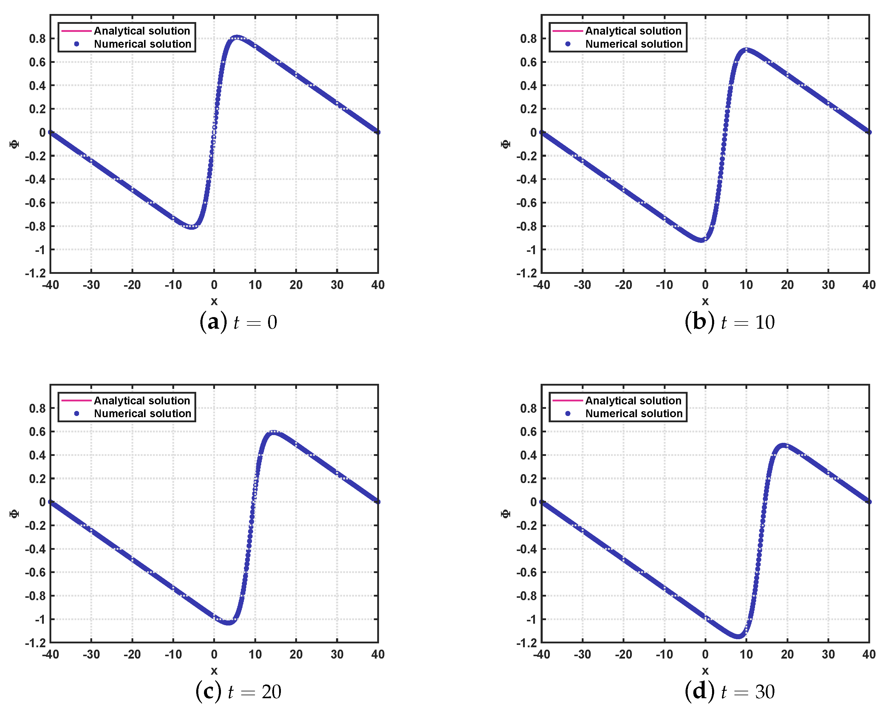
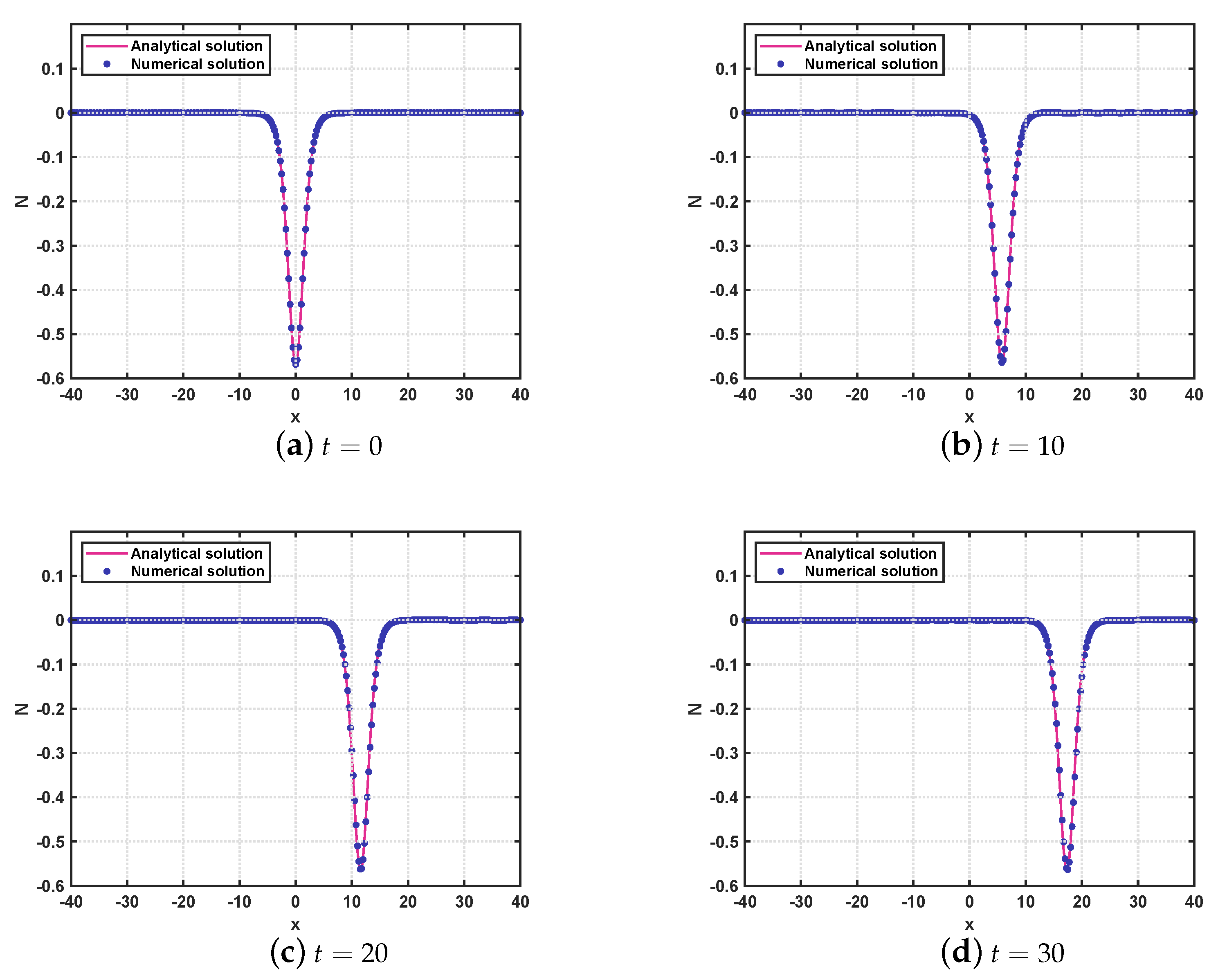
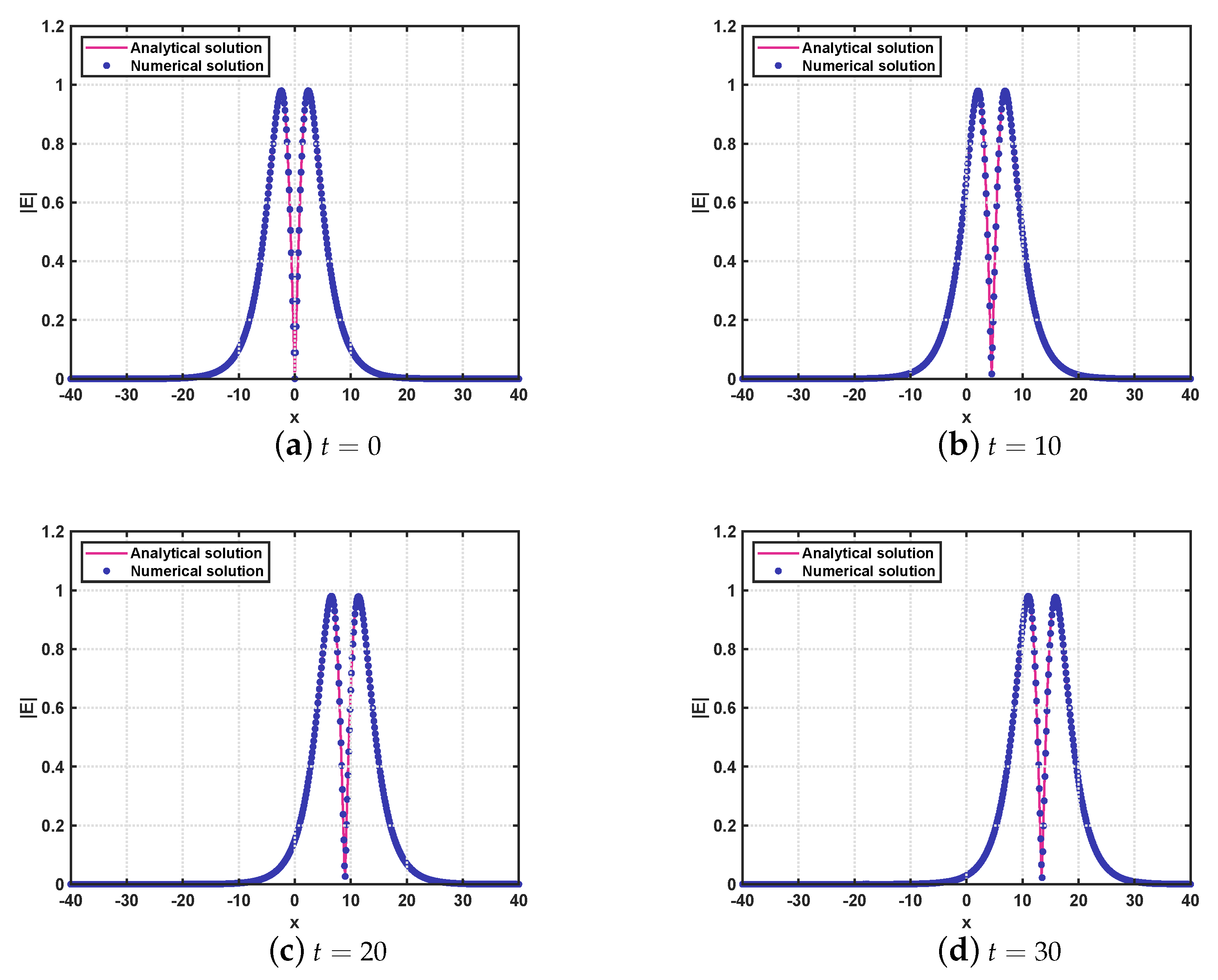
Taking the time interval J ¯ = 0 , 10 , the fixed time step τ = τ C 4 = 1 / 300 , and changed space step length h = 1 / 2 , 1 / 4 , 1 / 8 , we obtain the convergence data of the standard nonlinear finite element method and the fast TT-M finite element method in Table 3, which implies that the fast TT-M FE method can maintain the same calculation accuracy as the standard finite element method and reduce the calculation time to a great extent. A similar case can also be seen in the space-time convergence calculation data in Table 4. By taking the time interval J ¯ = 0 , 30 and time step size τ = τ C 4 = 1 100 , we more vividly show the dynamic behavior of the numerical solution in Figure 1, Figure 2 and Figure 3, from which it is easy to see the performance behavior of the numerical images of the three functions at each fixed time point, and we can also observe the moving process, the behavior performance change of the numerical solution and the change of spatial position from t = 0 , t = 10 , t = 20 to t = 30 .
For Case 2, we choose
γ = 1 , λ = 1 , α = 1 2 , θ = 3 2 , ω = 1 12 , m = 1 3 , δ = 1 5 , Ω ¯ = 40 , 40 .
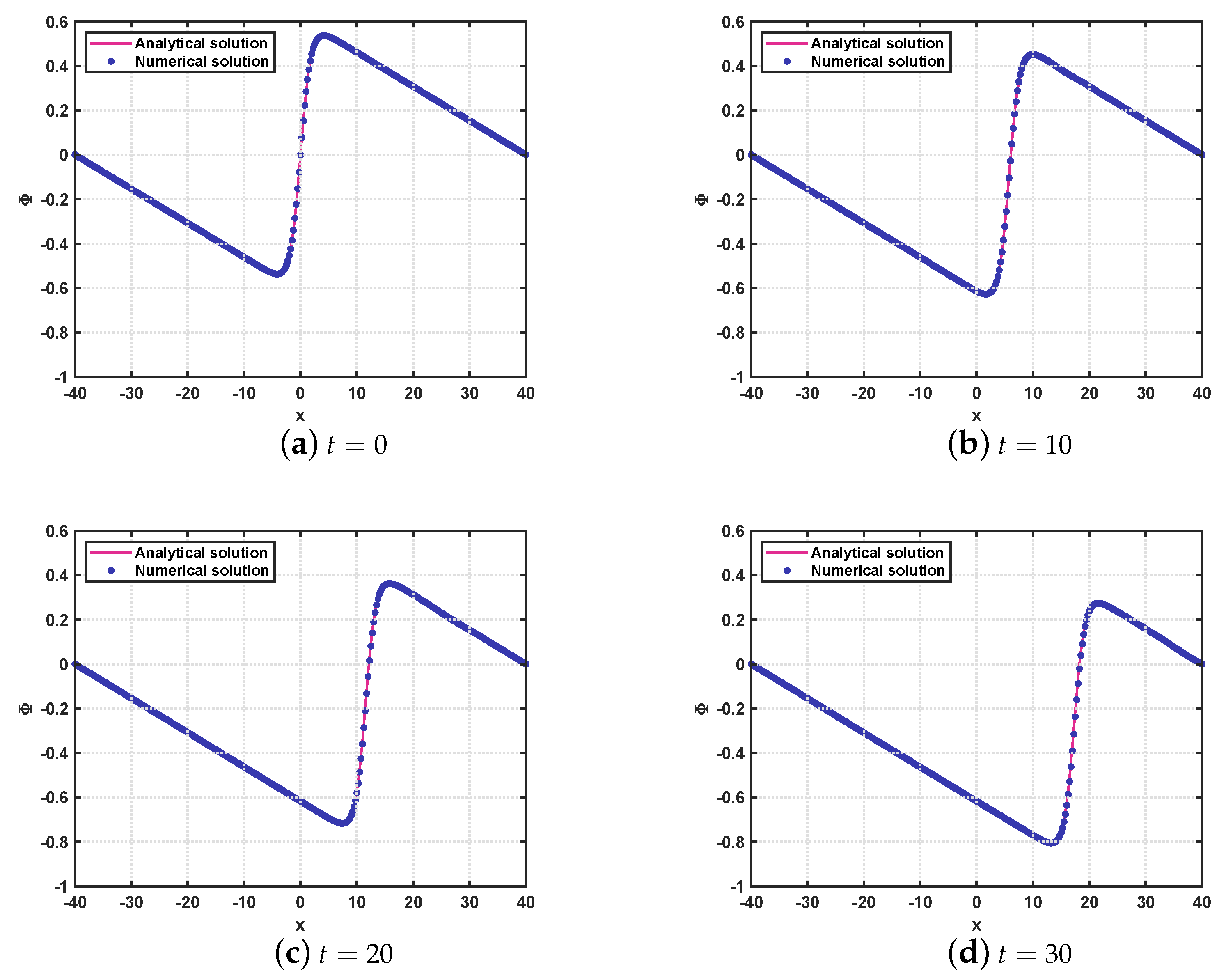
When taking the time interval J ¯ = 0 , 10 and the same space-time step length as Case 1, we obtain the space and space-time convergence data in Table 5 and Table 6. Similarly, compared with the standard FE method, the TT-M FE algorithm can maintain the calculation accuracy and improve the calculation efficiency. In Figure 4, Figure 5 and Figure 6, we also show the performance behavior of the numerical solution when taking the time interval J ¯ = 0 , 30 and τ = τ C 4 = 1 100 .
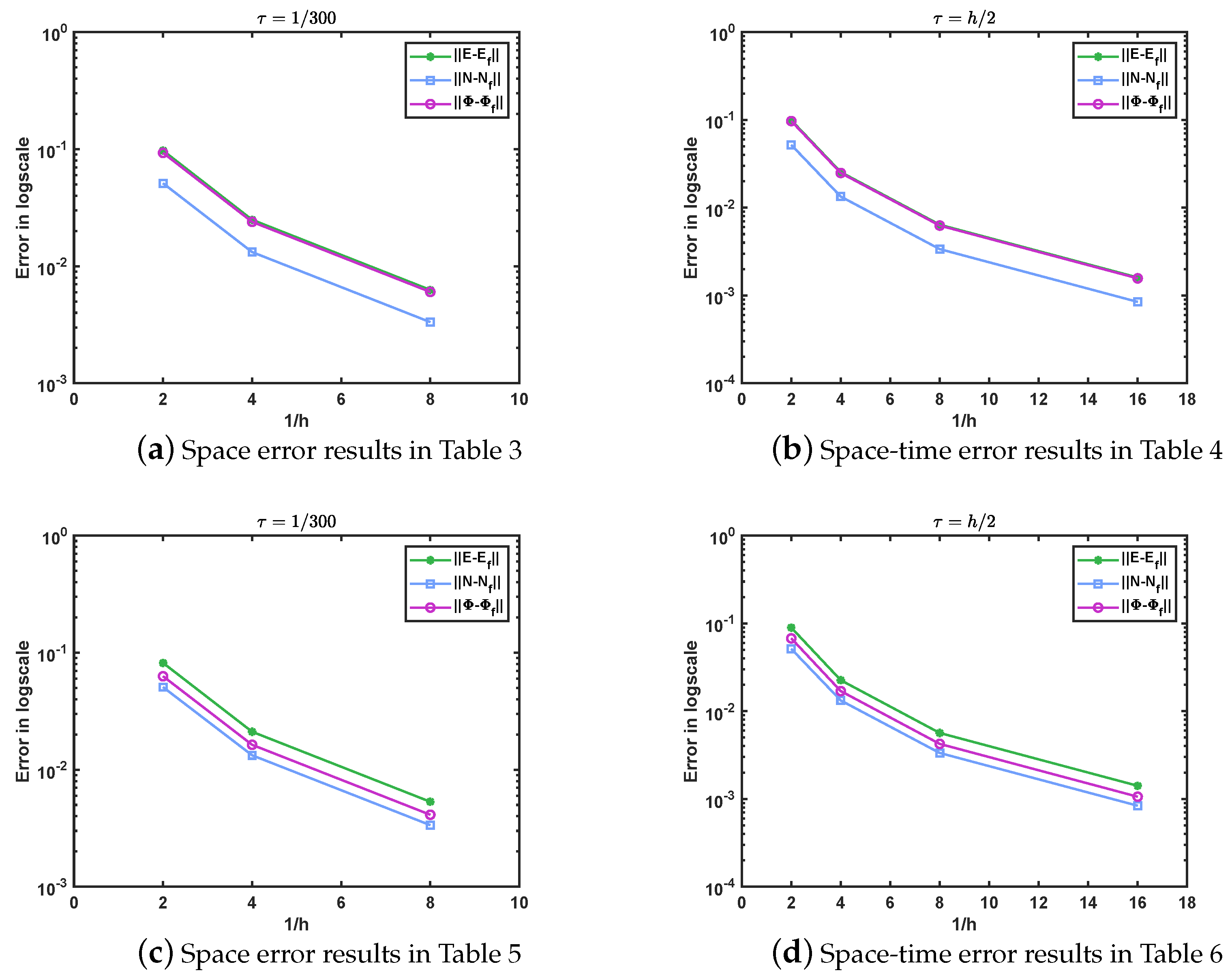
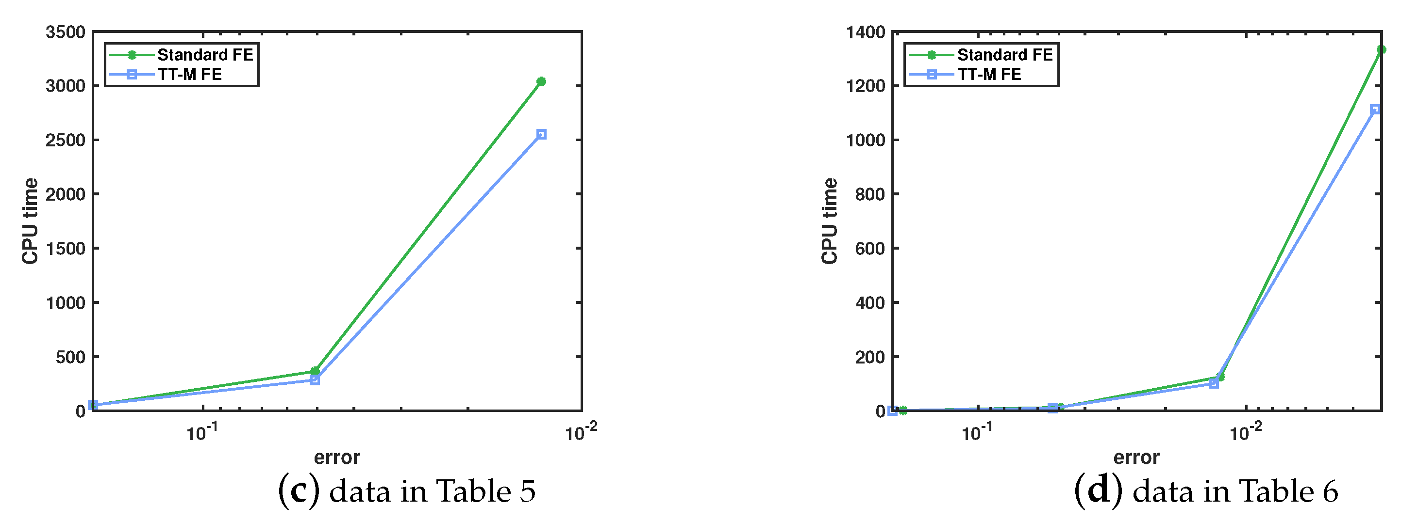
In Figure 7, we depict the relationship between errors in the log scale based on the data computed in Table 3, Table 4, Table 5 and Table 6 and 1 / h , from which one can clearly see that as the parameter 1 / h becomes larger, the errors becomes smaller. In Figure 8, where the error-axis is in the log scale, we show the comparison of performance of calculation time between the TT-M FE method and the standard FE method, which visually illustrates that the TT-M FE method has the advantage of saving computing time.

6. Conclusions

In this article, the coupled Schrödinger–Boussinesq equations are numerically solved by using the FE method combined with the TT-M fast algorithm so as to improve the calculation speed and reduce the calculation time. A theoretical analysis on the TT-M FE system is derived. In numerical experiments, the effectiveness and correctness of the algorithm are confirmed by a significant amount of calculation data, the dynamic behaviors of the numerical solutions are shown by several numerical images, and the advantage of the calculation speed of the algorithm is reflected by making a comparison with the standard nonlinear Galerkin FE method.
In the future, we will apply the TT-M FE method to two- or three-dimensional coupled Schrödinger–Boussinesq models, nonlinear fractional Schrödinger equations [34,35,36,37,38,39,40,41] and the coupled nonlinear Schrödinger equations [42,43,44], and also investigate the method’s conservation properties.

Author Contributions

Conceptualization, J.T.; methodology, Y.L.; software, Z.S.; validation, Y.L. and H.L.; formal analysis, J.T.; writing—original draft preparation, J.T. and Z.S.; writing—review and editing, Y.L. and H.L.; funding acquisition, Z.S., Y.L. and H.L. All authors have read and agreed to the published version of the manuscript.

Funding

This work is supported by the Natural Science Foundation of Inner Mongolia (2020MS01003; 2021MS01018), Program for Innovative Research Team in Universities of Inner Mongolia Autonomous Region (NMGIRT2207), and National Innovation Project (202110126023).

Institutional Review Board Statement

Not applicable.

Informed Consent Statement

Not applicable.

Data Availability Statement

All the data were computed using our algorithm.

Acknowledgments

We are grateful to the three anonymous reviewers and editors for their valuable suggestions and comments.

Conflicts of Interest

The authors declare no conflict of interest.

References

  1. Yajima, N.; Satsuma, J. Soliton solutions in a diatomic lattice system. Prog. Theor. Phys. 1979, 62, 370–378. [Google Scholar] [CrossRef]
  2. Rao, N.N. Coupled scalar field equations for nonlinear wave modulations in dispersive media. Pramana J. Phys. 1996, 46, 161–202. [Google Scholar] [CrossRef]
  3. Liao, F.; Zhang, L.M.; Wang, S.S. Numerical analysis of cubic orthogonal spline collocation methods for the coupled Schrödinger-Boussinesq equations. Appl. Numer. Math. 2017, 119, 194–212. [Google Scholar] [CrossRef]
  4. Guo, B.L.; Du, X.Y. The behavior of attractors for damped Schrödinger-Boussinesq equation. Commun. Nonlinear Sci. Numer. Simul. 2001, 6, 54–60. [Google Scholar] [CrossRef]
  5. Bilige, S.; Chaolu, T.; Wang, X.M. Application of the extended simplest equation method to the coupled Schrödinger-Boussinesq equation. Appl. Math. Comput. 2013, 224, 517–523. [Google Scholar] [CrossRef]
  6. Guo, B.L. The global solution of the system of equations for complex Schrödinger field coupled with Boussinesq type self-consistent field. Acta Math. Sin. 1983, 26, 295–306. (In Chinese) [Google Scholar] [CrossRef]
  7. Li, Y.S.; Chen, Q.Y. Finite dimensional global attractor for dissipative Schrödinger-Boussinesq equations. J. Math. Anal. Appl. 1997, 205, 107–132. [Google Scholar] [CrossRef] [Green Version]
  8. Guo, B.L.; Chen, F.X. Finite dimensional behavior of global attractors for weakly damped nonlinear Schrödinger-Boussinesq equations. Physica D 1996, 93, 101–118. [Google Scholar]
  9. Farah, L.G.; Pastor, A. On the periodic Schrödinger-Boussinesq system. J. Math. Anal. Appl. 2010, 368, 330–349. [Google Scholar] [CrossRef] [Green Version]
  10. Guo, B.L.; Du, X.Y. Existence of the periodic solution for the weakly damped Schrödinger-Boussinesq equation. J. Math. Anal. Appl. 2001, 262, 453–472. [Google Scholar] [CrossRef] [Green Version]
  11. Hon, Y.V.; Fan, E.G. A series of exact solutions for coupled Higgs field equation and coupled Schrödinger-Boussinesq equation. Nonlinear Anal. 2009, 71, 3501–3508. [Google Scholar] [CrossRef]
  12. Rao, N.N. Exact solutions of coupled scalar field equations. J. Phys. A Math. Gen. 1989, 22, 4813–4825. [Google Scholar] [CrossRef]
  13. Xia, Y.R.; Li, Z.B. Exact explicit solutions of the nonlinear Schrödinger equation coupled to the Boussinesq equation. Acta Math. Sci. 2003, 23, 453–460. [Google Scholar]
  14. Liao, F.; Zhang, L.M.; Wang, S.S. Time-splitting combined with exponential wave integrator Fourier pseudospectral method for Schrödinger-Boussinesq system. Commun. Nonlinear Sci. Numer. Simulat. 2018, 55, 93–104. [Google Scholar] [CrossRef]
  15. Zhang, L.M.; Bai, D.M.; Wang, S.S. Numerical analysis for a conservative difference scheme to solve the Schrödinger-Boussinesq equation. J. Comput. Appl. Math. 2011, 235, 4899–4915. [Google Scholar] [CrossRef] [Green Version]
  16. Liao, F.; Zhang, L.M. Conservative compact finite difference scheme for the coupled Schrödinger-Boussinesq equation. Numer. Meth. Part. Differ. Equ. 2016, 32, 1667–1688. [Google Scholar] [CrossRef]
  17. Deng, D.W.; Wu, Q. Analysis of the linearly energy- and mass-preserving finite difference methods for the coupled Schrödinger-Boussinesq equations. Appl. Numer. Math. 2021, 170, 14–38. [Google Scholar] [CrossRef]
  18. Zheng, J.D.; Xiang, X.M. The finite element analysis for the equation system coupling the complex Schrödinger and real Boussinesq fields. Math. Numer. Sin. 1987, 9, 133–143. [Google Scholar]
  19. Bai, D.M.; Zhang, L.M. The quadratic B-spline finite element method for the coupled Schrödinger-Boussinesq equations. Int. J. Comput. Math. 2011, 88, 1714–1729. [Google Scholar] [CrossRef]
  20. Huang, L.Y.; Jiao, Y.D.; Liang, D.M. Multi-symplectic scheme for the coupled Schrödinger-Boussinesq equations. Chin. Phys. B 2013, 7, 070201. [Google Scholar] [CrossRef]
  21. Cai, J.X.; Chen, J.; Yang, B. Efficient energy-preserving wavelet collocation schemes for the coupled nonlinear Schrödinger-Boussinesq system. Appl. Math. Comput. 2019, 357, 1–11. [Google Scholar] [CrossRef]
  22. Guo, B.L.; Chen, G.N. The convergence of Galerkin-Fourier method for equation of Schrödinger-Boussinesq field. J. Comput. Math. 1984, 2, 344–355. [Google Scholar]
  23. Liu, Y.; Yu, Z.D.; Li, H.; Liu, F.W.; Wang, J.F. Time two-mesh algorithm combined with finite element method for time fractional water wave model. Int. J. Heat Mass Transf. 2018, 120, 1132–1145. [Google Scholar] [CrossRef]
  24. Yin, B.L.; Liu, Y.; Li, H.; He, S. Fast algorithm based on TT-M FE system for space fractional Allen-Cahn equations with smooth and non-smooth solutions. J. Comput. Phys. 2019, 379, 351–372. [Google Scholar] [CrossRef] [Green Version]
  25. Liu, Y.; Fan, E.Y.; Yin, B.L.; Li, H.; Wang, J.F. TT-M finite element algorithm for a two-dimensional space fractional Gray-Scott model. Comput. Math. Appl. 2020, 80, 1793–1809. [Google Scholar] [CrossRef]
  26. Wen, C.; Liu, Y.; Yin, B.L.; Li, H.; Wang, J.F. Fast second-order time two-mesh mixed finite element method for a nonlinear distributed-order sub-diffusion model. Numer. Algorithms 2021, 88, 523–553. [Google Scholar] [CrossRef]
  27. Wang, D.X.; Du, Q.Q.; Zhang, J.W.; Jia, H.E. A fast time two-mesh algorithm for Allen-Cahn equation. Bull. Malays. Math. Sci. Soc. 2020, 43, 2417–2441. [Google Scholar] [CrossRef]
  28. Qiu, W.L.; Xu, D.; Guo, J.; Zhou, J. A time two-grid algorithm based on finite difference method for the two-dimensional nonlinear time-fractional mobile/immobile transport model. Numer. Algorithms 2020, 85, 39–58. [Google Scholar] [CrossRef]
  29. Niu, Y.X.; Liu, Y.; Li, H.; Liu, F.W. Fast high-order compact difference scheme for the nonlinear distributed-order fractional Sobolev model appearing in porous media. 2021; submitted. [Google Scholar]
  30. Tutueva, A.; Karimov, T.; Butusov, D. Semi-implicit and semi-explicit Adams-Bashforth-Moulton methods. Mathematics 2020, 8, 780. [Google Scholar] [CrossRef]
  31. Tutueva, A.; Butusov, D. Avoiding dynamical degradation in computer simulation of chaotic systems using semi-explicit integration: Rössler oscillator case. Fract. Fract. 2021, 5, 214. [Google Scholar] [CrossRef]
  32. Thomee, V. Galerkin Finite Element Method for Parabolic Problems; Springer: Berlin/Heidelberg, Germany, 1984. [Google Scholar]
  33. Wen, C.; Wang, J.F.; Liu, Y.; Li, H.; Fang, Z.C. Unconditionally optimal time two-mesh mixed finite element algorithm for a nonlinear distributed-order fourth-order equation. 2022; submitted. [Google Scholar]
  34. Li, M.; Huang, C.M.; Wang, P.D. Galerkin finite element method for nonlinear fractional Schrödinger equations. Numer. Algorithms 2017, 74, 499–525. [Google Scholar] [CrossRef]
  35. Li, D.F.; Wang, J.L.; Zhang, J.W. Unconditionally convergent L1-Galerkin FEMs for nonlinear time-fractional Schrödinger equations. SIAM J. Sci. Comput. 2017, 39, A3067–A3088. [Google Scholar] [CrossRef]
  36. Yin, B.L.; Wang, J.F.; Liu, Y.; Li, H. A structure preserving difference scheme with fast algorithms for high dimensional nonlinear space-fractional Schrödinger equations. J. Comput. Phys. 2021, 425, 109869. [Google Scholar] [CrossRef]
  37. Liu, Q.; Zeng, F.H.; Li, C.P. Finite difference method for time-space-fractional Schrödinger equation. Int. J. Comput. Math. 2015, 92, 1439–1451. [Google Scholar] [CrossRef]
  38. Ran, M.; Zhang, C. Linearized Crank-Nicolson scheme for the nonlinear time-space fractional Schrödinger equations. J. Comput. Appl. Math. 2019, 355, 218–231. [Google Scholar] [CrossRef]
  39. Zheng, M.; Liu, F.; Jin, Z. The global analysis on the spectral collocation method for time fractional Schrödinger equation. Appl. Math. Comput. 2020, 365, 124689. [Google Scholar] [CrossRef]
  40. Wang, Y.; Mei, L.; Li, Q.; Bu, L. Split-step spectral Galerkin method for the two-dimensional nonlinear space-fractional Schrödinger equation. Appl. Numer. Math. 2019, 136, 257–278. [Google Scholar] [CrossRef]
  41. Zhang, H.; Jiang, X.; Wang, C.; Chen, S. Crank-Nicolson Fourier spectral methods for the space fractional nonlinear Schrödinger equation and its parameter estimation. Int. J. Comput. Math. 2019, 96, 238–263. [Google Scholar] [CrossRef]
  42. Wang, D.L.; Xiao, A.G.; Yang, W. A linearly implicit conservative difference scheme for the space fractional coupled nonlinear Schrödinger equations. J. Comput. Phys. 2014, 272, 644–655. [Google Scholar] [CrossRef]
  43. Iqbal, A.; Hamid, N.N.A.; Ismail, A.I.M.; Abbas, M. Galerkin approximation with quintic B-spline as basis and weight functions for solving second order coupled nonlinear Schrödinger equations. Math. Comput. Simulat. 2021, 187, 1–16. [Google Scholar] [CrossRef]
  44. Ma, Y.P.; Kong, L.H.; Hong, J.L.; Cao, Y. High-order compact splitting multisymplectic method for the coupled nonlinear Schrödinger equations. Comput. Math. Appl. 2011, 61, 319–333. [Google Scholar] [CrossRef]
Figure 1. Comparison between numerical solution | E f | () and analytical solution | E | () with τ = τ C 4 = 1 100 and h = 1 8 at different points in time for Case 1 of Example 2.
Axioms 11 00314 g001
Figure 2. Comparison between numerical solution N f () and analytical solution N () with τ = τ C 4 = 1 100 and h = 1 8 at different points in time for Case 1 of Example 2.
Axioms 11 00314 g002
Figure 3. Comparison between numerical solution Φ f () and analytical solution Φ () with τ = τ C 4 = 1 100 and h = 1 8 at different points in time for Case 1 of Example 2.
Axioms 11 00314 g003
Figure 4. Comparison between numerical solution | E f | () and analytical solution | E | () with τ = τ C 4 = 1 100 and h = 1 4 at different points in time for Case 2 of Example 2.
Axioms 11 00314 g004
Figure 5. Comparison between numerical solution N f () and analytical solution N () with τ = τ C 4 = 1 100 and h = 1 4 at different points in time for Case 2 of Example 2.
Axioms 11 00314 g005
Figure 6. Comparison between numerical solution Φ f () and analytical solution Φ () with τ = τ C 4 = 1 100 and h = 1 4 at different points in time for Case 2 of Example 2.
Axioms 11 00314 g006
Figure 7. Performances of errors in log scale based on the data calculated in Table 3, Table 4, Table 5 and Table 6.
Axioms 11 00314 g007
Figure 8. Comparison for the computing time between the TT-M FE method and the standard FE method based on the data in Table 3, Table 4, Table 5 and Table 6.
Axioms 11 00314 g008aAxioms 11 00314 g008b
Table 1. Space convergence results for Example 1 with τ C = 4 τ .
Standard FE Algorithm
( h , τ ) Ξ E h n ( τ , h ) Rate Ξ N h n ( τ , h ) Rate Ξ Φ h n ( τ , h ) RateCPU(s)
( π 20 , 1 3000 ) 1.5458 × 10 2 2.8961 × 10 2 6.7647 × 10 2 1.77
( π 40 , 1 3000 ) 3.8651 × 10 3 1.99977.3072 × 10 3 1.98671.7086 × 10 2 1.98523.25
( π 80 , 1 3000 ) 9.6635 × 10 4 1.99991.8335 × 10 3 1.99484.2815 × 10 3 1.99668.83
( π 160 , 1 3000 ) 2.4162 × 10 4 1.99984.5865 × 10 4 1.99911.0709 × 10 3 1.999353.00
( π 320 , 1 3000 ) 6.0442 × 10 5 1.99911.1459 × 10 4 2.00092.6761 × 10 4 2.0006317.05
TT-M FE Algorithm
( h , τ ) Ξ E f n ( τ , h ) Rate Ξ N f n ( τ , h ) Rate Ξ Φ f n ( τ , h ) RateCPU(s)
( π 20 , 1 3000 ) 1.5458 × 10 2 2.8962 × 10 2 6.7647 × 10 2 1.77
( π 40 , 1 3000 ) 3.8651 × 10 3 1.99977.3073 × 10 3 1.98671.7086 × 10 2 1.98523.07
( π 80 , 1 3000 ) 9.6632 × 10 4 1.99991.8336 × 10 3 1.99474.2816 × 10 3 1.99668.76
( π 160 , 1 3000 ) 2.4160 × 10 4 1.99994.5878 × 10 4 1.99881.0710 × 10 3 1.999153.56
( π 320 , 1 3000 ) 6.0414 × 10 5 1.99961.1472 × 10 4 1.99972.6779 × 10 4 1.9998282.96
Table 2. Space-time convergence results for Example 1 with τ = 1 π h and τ C = 4 τ .
Standard FE Algorithm
( h , τ ) Ξ E h n ( τ , h ) Rate Ξ N h n ( τ , h ) Rate Ξ Φ h n ( τ , h ) RateCPU(s)
( π 20 , 1 20 ) 1.5913 × 10 2 2.5619 × 10 2 6.2220 × 10 2 0.02
( π 40 , 1 40 ) 3.9807 × 10 3 1.99916.4235 × 10 3 1.99581.5737 × 10 2 1.98330.06
( π 80 , 1 80 ) 9.9505 × 10 4 2.00021.6056 × 10 3 2.00023.9462 × 10 3 1.99560.31
( π 160 , 1 160 ) 2.4882 × 10 4 1.99974.0175 × 10 4 1.99889.8720 × 10 4 1.99913.13
( π 320 , 1 320 ) 6.2204 × 10 5 2.00001.0039 × 10 4 2.00072.4666 × 10 4 2.000836.44
( π 640 , 1 640 ) 1.5551 × 10 5 2.00002.5105 × 10 5 1.99966.1688 × 10 5 1.9994443.56
TT-M FE Algorithm
( h , τ ) Ξ E f n ( τ , h ) Rate Ξ N f n ( τ , h ) Rate Ξ Φ f n ( τ , h ) RateCPU(s)
( π 20 , 1 20 ) 1.5984 × 10 2 2.8722 × 10 2 6.7901 × 10 2 0.04
( π 40 , 1 40 ) 3.9951 × 10 3 2.00037.1917 × 10 3 1.99781.7111 × 10 2 1.98850.05
( π 80 , 1 80 ) 9.9906 × 10 4 1.99961.7973 × 10 3 2.00054.2867 × 10 3 1.99700.26
( π 160 , 1 160 ) 2.4977 × 10 4 2.00004.4967 × 10 4 1.99891.0721 × 10 3 1.99952.85
( π 320 , 1 320 ) 6.2444 × 10 5 2.00001.1240 × 10 4 2.00032.6806 × 10 4 1.999831.30
( π 640 , 1 640 ) 1.5611 × 10 5 2.00002.8100 × 10 5 1.99996.7016 × 10 5 2.0000343.06
Table 3. Space convergence results for Example 2 in Case 1 with τ C = 4 τ .
Standard FE Algorithm
( h , τ ) Ξ E h n ( τ , h ) Rate Ξ N h n ( τ , h ) Rate Ξ Φ h n ( τ , h ) RateCPU(s)
( 1 2 , 1 300 ) 9.7274 × 10 2 5.1130 × 10 2 9.3026 × 10 2 62.39
( 1 4 , 1 300 ) 2.4921 × 10 2 1.96471.3201 × 10 2 1.95352.3933 × 10 2 1.9586385.42
( 1 8 , 1 300 ) 6.2693 × 10 3 1.99103.3276 × 10 3 1.98816.0274 × 10 3 1.98943093.74
TT-M FE Algorithm
( h , τ ) Ξ E f n ( τ , h ) Rate Ξ N f n ( τ , h ) Rate Ξ Φ f n ( τ , h ) RateCPU(s)
( 1 2 , 1 300 ) 9.7274 × 10 2 5.1130 × 10 2 9.3027 × 10 2 51.98
( 1 4 , 1 300 ) 2.4921 × 10 2 1.96471.3201 × 10 2 1.95352.3934 × 10 2 1.9586297.16
( 1 8 , 1 300 ) 6.2698 × 10 3 1.99093.3279 × 10 3 1.98806.0284 × 10 3 1.98922521.57
Table 4. Space-time convergence results for Example 2 in Case 1 with τ = 1 2 h and τ C = 4 τ .
Standard FE Algorithm
( h , τ ) Ξ E h n ( τ , h ) Rate Ξ N h n ( τ , h ) Rate Ξ Φ h n ( τ , h ) RateCPU(s)
( 1 2 , 1 4 ) 9.6515 × 10 2 4.9930 × 10 2 9.0913 × 10 2 1.09
( 1 4 , 1 8 ) 2.4741 × 10 2 1.96381.2908 × 10 2 1.95162.3431 × 10 2 1.956113.35
( 1 8 , 1 16 ) 6.2254 × 10 3 1.99073.2549 × 10 3 1.98765.9038 × 10 3 1.9887137.33
( 1 16 , 1 32 ) 1.5589 × 10 3 1.99778.1550 × 10 4 1.99691.4789 × 10 3 1.99712000.16
TT-M FE Algorithm
( h , τ ) Ξ E f n ( τ , h ) Rate Ξ N f n ( τ , h ) Rate Ξ Φ f n ( τ , h ) RateCPU(s)
( 1 2 , 1 4 ) 9.9179 × 10 2 5.1934 × 10 2 9.7061 × 10 2 1.05
( 1 4 , 1 8 ) 2.5426 × 10 2 1.96371.3388 × 10 2 1.95582.4873 × 10 2 1.96439.97
( 1 8 , 1 16 ) 6.3972 × 10 3 1.99083.3734 × 10 3 1.98866.2584 × 10 3 1.9907112.46
( 1 16 , 1 32 ) 1.6019 × 10 3 1.99778.4504 × 10 4 1.99711.5671 × 10 3 1.99771246.46
Table 5. Space convergence results for Example 2 in Case 2 with τ C = 4 τ .
Standard FE Algorithm
( h , τ ) Ξ E h n ( τ , h ) Rate Ξ N h n ( τ , h ) Rate Ξ Φ h n ( τ , h ) RateCPU(s)
( 1 2 , 1 300 ) 8.1725 × 10 2 5.0737 × 10 2 6.2883 × 10 2 49.55
( 1 4 , 1 300 ) 2.1093 × 10 2 1.95401.3275 × 10 2 1.93431.6315 × 10 2 1.9465364.28
( 1 8 , 1 300 ) 5.3172 × 10 3 1.98803.3580 × 10 3 1.98304.1181 × 10 3 1.98613037.39
TT-M FE Algorithm
( h , τ ) Ξ E f n ( τ , h ) Rate Ξ N f n ( τ , h ) Rate Ξ Φ f n ( τ , h ) RateCPU(s)
( 1 2 , 1 300 ) 8.1726 × 10 2 5.0738 × 10 2 6.2884 × 10 2 53.02
( 1 4 , 1 300 ) 2.1094 × 10 2 1.95401.3276 × 10 2 1.93431.6315 × 10 2 1.9465284.42
( 1 8 , 1 300 ) 5.3179 × 10 3 1.98793.3584 × 10 3 1.98294.1189 × 10 3 1.98592551.25
Table 6. Space-time convergence results for Example 2 in Case 2 with τ = 1 2 h and τ C = 4 τ .
Standard FE Algorithm
( h , τ ) Ξ E h n ( τ , h ) Rate Ξ N h n ( τ , h ) Rate Ξ Φ h n ( τ , h ) RateCPU(s)
( 1 2 , 1 4 ) 8.2622 × 10 2 4.8094 × 10 2 5.9645 × 10 2 1.14
( 1 4 , 1 8 ) 2.1377 × 10 2 1.95051.2609 × 10 2 1.93141.5536 × 10 2 1.940812.62
( 1 8 , 1 16 ) 5.3921 × 10 3 1.98713.1915 × 10 3 1.98213.9261 × 10 3 1.9845125.44
( 1 16 , 1 32 ) 1.3509 × 10 3 1.99708.0053 × 10 4 1.99529.8422 × 10 4 1.99611333.25
TT-M FE Algorithm
( h , τ ) Ξ E f n ( τ , h ) Rate Ξ N f n ( τ , h ) Rate Ξ Φ f n ( τ , h ) RateCPU(s)
( 1 2 , 1 4 ) 8.9536 × 10 2 5.1280 × 10 2 6.7564 × 10 2 0.99
( 1 4 , 1 8 ) 2.2549 × 10 2 1.98941.3252 × 10 2 1.95211.6945 × 10 2 1.99549.36
( 1 8 , 1 16 ) 5.6463 × 10 3 1.99773.3410 × 10 3 1.98794.2393 × 10 3 1.9989100.56
( 1 16 , 1 32 ) 1.4121 × 10 3 1.99958.3702 × 10 4 1.99701.0600 × 10 3 1.99981112.97
Publisher’s Note: MDPI stays neutral with regard to jurisdictional claims in published maps and institutional affiliations.