
New Robust Estimators for Handling Multicollinearity and Outliers in the Poisson Model: Methods, Simulation and Applications


Abstract
:1. Introduction
2. Methodology
2.1. Poisson One-Parameter Regression Estimators
2.2. Robust Poisson Ridge Regression Estimator
2.3. Proposed Robust Poisson One-Parameter Regression Estimators
2.4. Superiority of Proposed Estimators
2.5. Selection of Biasing Parameters
- The suggested for the PRR estimator is:
- The suggested for the RPRR estimator is:
- The suggested for the PL estimator is:
- The suggested for the RPL estimator is:
- The two suggested for the PKL estimator are and
- The two suggested for the RPKL estimator are and
- Three are suggested for the PMKL estimator: , , and
- The three suggested for the RPMKL estimator are , and
3. Simulation Study
3.1. Simulation Design
3.2. Simulation Results
- The PML performance was the worst of the given estimators in the existence of both outliers and multicollinearity problems, as expected;
- The estimators’ AMSE values were increased in the case of the multicollinearity degree (), explanatory variables number (p), and outlier percentage ();
- The estimators’ AMSE values were decreased in the case of the sample size (n) being increased, when the other factors were fixed;
- When only the multicollinearity problem existed in the model (as in Table A1, Table A2 and Table A3 or when no outliers existed, i.e., ), the non-robust estimators (PML, PRR, PL, PKL, and PMKL) were better than the corresponding robust estimators (RPML, RPRR, RPL, RPKL, and RPMKL) for all , p, and n values;
- For n = 75, 100, = −1, τ = 0% and ρ = 0.90, 0.95, the PKL.1 AMSE values were the lowest among all models, and for n = 75, 100, β1 = −1, τ = 10% and ρ = 0.90, the RPKL.1 AMSE values were the lowest among all models;
- When , the PMKL estimator, and in particular, the PMKL.1 was the best, followed by the PKL, and in particular, the PKL.1 in most situations;
- In addition, when , the RPMKL estimator was the best, particularly the RPMKL.1, followed by the RPKL estimator, particularly the RPKL.1 in most situations;
- Finally, the PMKL estimator achieved the best performance among all given estimators when only the multicollinearity problem existed in the model. If both outliers and multicollinearity problems existed in the model, the RPMKL estimator achieved the best performance among all given estimators in most situations.
4. Empirical Applications
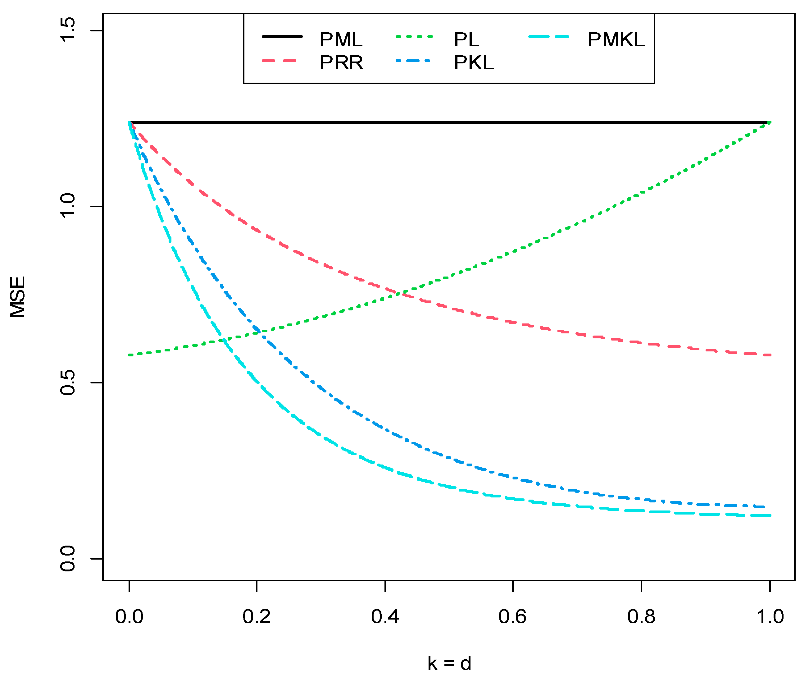
4.1. Aircraft Damage Data
- The PML estimator performed the worst among all given estimators;
- The robust estimators achieved a better performance than the corresponding non-robust estimators;
- The PMKL performed better in general, followed by the PKL, and then the other non-robust estimators. Additionally, the RPMKL achieved a better performance in general, followed by the RPKL and then the other robust estimators;
- Finally, the RPMKL, particularly the RPMKL.1 estimator was the best, which had the lowest AMSE value.
- Since the condition was satisfied, then the RPL estimator was better than the RPML estimator;
- Since the condition was satisfied, then the RPKL estimator was better than the RPML estimator;
- Since the condition was satisfied, then the RPMKL estimator was better than the RPML estimator;
- Since the condition was satisfied, then the RPL estimator was better than the RPRR estimator;
- Since the condition was satisfied, then the RPKL estimator was better than the RPRR estimator;
- Since the condition was satisfied, then the RPMKL estimator was better than the RPRR estimator;
- Since the condition was satisfied, then the RPKL estimator was better than the RPL estimator;
- Since the condition was satisfied, then the RPMKL estimator was better than the RPL estimator;
- Since the condition was satisfied, then the RPMKL estimator was better than the RPKL estimator.
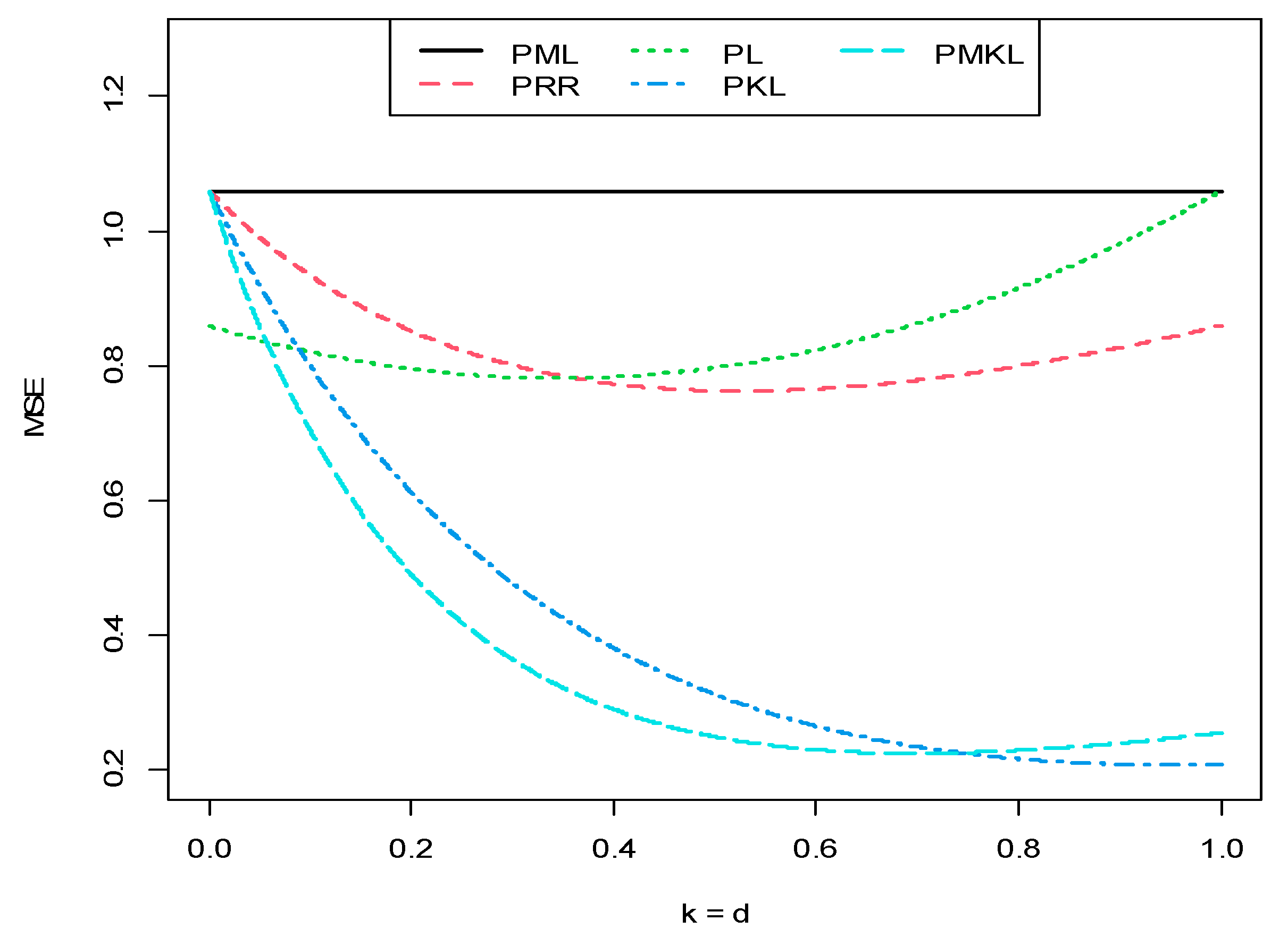
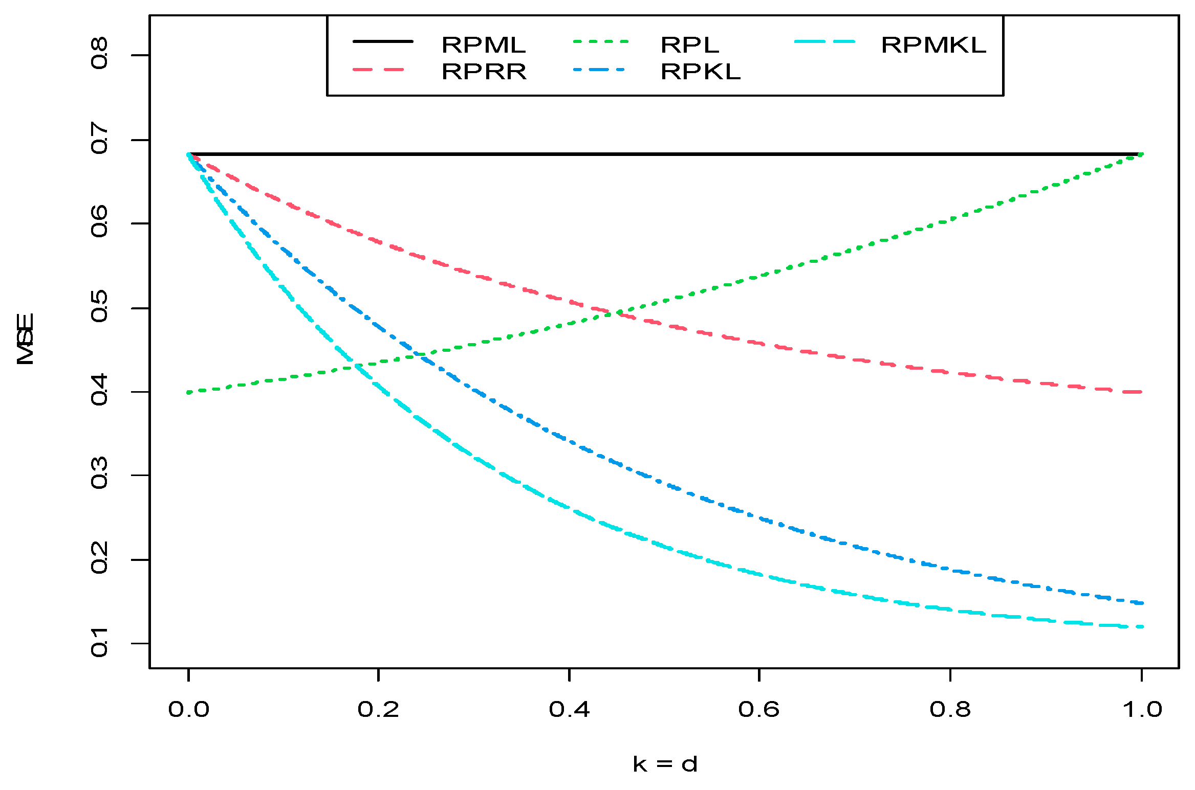
4.2. Somerville Lake Data
- The PML performed worst among all given estimators;
- The robust estimators achieved a better performance than the corresponding non-robust estimators;
- The PMKL achieved a better performance in general, followed by the PKL, and then the other non-robust estimators. Additionally, the RPMKL achieved a better performance in general, followed by the RPKL, and then the other robust estimators;
- Finally, the RPMKL, particularly the RPMKL.1 estimator was the best, which had the lowest AMSE value.
- Since the condition was satisfied, then the RPL estimator was better than the RPML estimator;
- Since the condition was satisfied, then the RPKL estimator was better than the RPML estimator;
- Since the condition was satisfied, then the RPMKL estimator was better than the RPML estimator;
- Since the condition was satisfied, then the RPL estimator was better than the RPRR estimator;
- Since the condition was satisfied, then the RPKL estimator was better than the RPRR estimator;
- Since the condition was satisfied, then the RPMKL estimator was better than the RPRR estimator;
- Since the condition was satisfied, then the RPKL estimator was better than the RPL estimator;
- Since the condition was satisfied, then the RPMKL estimator was better than the RPL estimator;
- Since the condition was satisfied, then the RPMKL estimator was better than the RPKL estimator.
5. Conclusions
Author Contributions
Funding
Data Availability Statement
Acknowledgments
Conflicts of Interest
Appendix A

| Non-Robust Estimators | Robust Estimators | ||||||||||||||||
|---|---|---|---|---|---|---|---|---|---|---|---|---|---|---|---|---|---|
| p | n | PML | PRR | PL | PKL.1 | PKL.2 | PMKL.1 | PMKL.2 | PMKL.3 | RPML | RPRR | RPL | RPKL.1 | RPKL.2 | RPMKL.1 | RPMKL.2 | RPMKL.3 |
| β1 = −1 | |||||||||||||||||
| 2 | 75 | 0.3623 | 0.1756 | 0.2830 | 0.1090 | 0.2078 | 0.1359 | 0.1701 | 0.1897 | 0.7051 | 0.2091 | 0.4876 | 0.1912 | 0.2728 | 0.2390 | 0.2066 | 0.2410 |
| 100 | 0.1933 | 0.1304 | 0.1708 | 0.1049 | 0.1488 | 0.1157 | 0.1352 | 0.1422 | 0.3022 | 0.1732 | 0.2531 | 0.1347 | 0.2055 | 0.1635 | 0.1788 | 0.1925 | |
| 200 | 0.0958 | 0.0794 | 0.0898 | 0.0689 | 0.0840 | 0.0656 | 0.0797 | 0.0820 | 0.1408 | 0.1073 | 0.1275 | 0.0862 | 0.1152 | 0.0810 | 0.1061 | 0.1109 | |
| 300 | 0.0445 | 0.0409 | 0.0431 | 0.0383 | 0.0418 | 0.0370 | 0.0408 | 0.0413 | 0.0687 | 0.0604 | 0.0652 | 0.0544 | 0.0622 | 0.0512 | 0.0597 | 0.0610 | |
| 6 | 75 | 0.7520 | 0.4799 | 0.5620 | 0.2970 | 0.4489 | 0.2230 | 0.3606 | 0.4072 | 1.1707 | 0.6060 | 0.8324 | 0.3197 | 0.6071 | 0.2366 | 0.4662 | 0.5402 |
| 100 | 0.2071 | 0.1833 | 0.1896 | 0.1665 | 0.1809 | 0.1579 | 0.1733 | 0.1771 | 0.2714 | 0.2313 | 0.2447 | 0.2059 | 0.2315 | 0.1963 | 0.2215 | 0.2263 | |
| 200 | 0.1174 | 0.1095 | 0.1113 | 0.1026 | 0.1081 | 0.0972 | 0.1042 | 0.1063 | 0.1657 | 0.1513 | 0.1541 | 0.1388 | 0.1477 | 0.1293 | 0.1405 | 0.1444 | |
| 300 | 0.0918 | 0.0882 | 0.0876 | 0.0848 | 0.0851 | 0.0818 | 0.0822 | 0.0838 | 0.1293 | 0.1216 | 0.1214 | 0.1145 | 0.1175 | 0.1086 | 0.1125 | 0.1152 | |
| β1 = 0 | |||||||||||||||||
| 2 | 75 | 0.0930 | 0.0829 | 0.0824 | 0.0735 | 0.0773 | 0.0658 | 0.0708 | 0.0743 | 0.1304 | 0.1101 | 0.1093 | 0.0918 | 0.0990 | 0.0784 | 0.0872 | 0.0936 |
| 100 | 0.0573 | 0.0540 | 0.0536 | 0.0508 | 0.0515 | 0.0480 | 0.0489 | 0.0503 | 0.0778 | 0.0716 | 0.0709 | 0.0659 | 0.0669 | 0.0611 | 0.0625 | 0.0649 | |
| 200 | 0.0304 | 0.0292 | 0.0291 | 0.0280 | 0.0285 | 0.0269 | 0.0276 | 0.0281 | 0.0473 | 0.0443 | 0.0442 | 0.0415 | 0.0427 | 0.0389 | 0.0406 | 0.0418 | |
| 300 | 0.0174 | 0.0170 | 0.0170 | 0.0167 | 0.0168 | 0.0164 | 0.0166 | 0.0167 | 0.0248 | 0.0241 | 0.0240 | 0.0233 | 0.0236 | 0.0226 | 0.0230 | 0.0234 | |
| 6 | 75 | 0.1373 | 0.1290 | 0.1287 | 0.1211 | 0.1247 | 0.1141 | 0.1191 | 0.1221 | 0.1779 | 0.1649 | 0.1645 | 0.1526 | 0.1582 | 0.1421 | 0.1496 | 0.1543 |
| 100 | 0.0882 | 0.0848 | 0.0847 | 0.0814 | 0.0832 | 0.0784 | 0.0808 | 0.0821 | 0.1164 | 0.1104 | 0.1103 | 0.1046 | 0.1076 | 0.0994 | 0.1035 | 0.1057 | |
| 200 | 0.0437 | 0.0427 | 0.0427 | 0.0417 | 0.0422 | 0.0408 | 0.0415 | 0.0419 | 0.0580 | 0.0562 | 0.0561 | 0.0544 | 0.0553 | 0.0528 | 0.0541 | 0.0548 | |
| 300 | 0.0162 | 0.0161 | 0.0161 | 0.0159 | 0.0160 | 0.0158 | 0.0159 | 0.0160 | 0.0221 | 0.0219 | 0.0219 | 0.0217 | 0.0218 | 0.0215 | 0.0216 | 0.0217 | |
| β1 = 1 | |||||||||||||||||
| 2 | 75 | 0.0591 | 0.0531 | 0.0565 | 0.0476 | 0.0542 | 0.0432 | 0.0520 | 0.0532 | 0.0799 | 0.0690 | 0.0753 | 0.0591 | 0.0710 | 0.0516 | 0.0670 | 0.0692 |
| 100 | 0.0225 | 0.0218 | 0.0222 | 0.0212 | 0.0219 | 0.0207 | 0.0217 | 0.0218 | 0.0338 | 0.0323 | 0.0331 | 0.0308 | 0.0325 | 0.0295 | 0.0319 | 0.0322 | |
| 200 | 0.0102 | 0.0101 | 0.0102 | 0.0099 | 0.0101 | 0.0098 | 0.0100 | 0.0101 | 0.0161 | 0.0157 | 0.0159 | 0.0153 | 0.0157 | 0.0150 | 0.0156 | 0.0157 | |
| 300 | 0.0063 | 0.0063 | 0.0063 | 0.0062 | 0.0063 | 0.0062 | 0.0063 | 0.0063 | 0.0088 | 0.0087 | 0.0088 | 0.0086 | 0.0088 | 0.0085 | 0.0087 | 0.0087 | |
| 6 | 75 | 0.1006 | 0.0945 | 0.0971 | 0.0886 | 0.0945 | 0.0835 | 0.0918 | 0.0933 | 0.1349 | 0.1244 | 0.1289 | 0.1146 | 0.1245 | 0.1062 | 0.1198 | 0.1224 |
| 100 | 0.0265 | 0.0262 | 0.0263 | 0.0259 | 0.0262 | 0.0257 | 0.0261 | 0.0262 | 0.0341 | 0.0336 | 0.0338 | 0.0331 | 0.0336 | 0.0327 | 0.0334 | 0.0335 | |
| 200 | 0.0106 | 0.0106 | 0.0106 | 0.0105 | 0.0106 | 0.0105 | 0.0105 | 0.0106 | 0.0133 | 0.0133 | 0.0133 | 0.0132 | 0.0133 | 0.0131 | 0.0132 | 0.0132 | |
| 300 | 0.0092 | 0.0092 | 0.0092 | 0.0092 | 0.0092 | 0.0091 | 0.0092 | 0.0092 | 0.0128 | 0.0127 | 0.0127 | 0.0126 | 0.0127 | 0.0125 | 0.0126 | 0.0127 | |
| Non-Robust Estimators | Robust Estimators | ||||||||||||||||
|---|---|---|---|---|---|---|---|---|---|---|---|---|---|---|---|---|---|
| p | n | PML | PRR | PL | PKL.1 | PKL.2 | PMKL.1 | PMKL.2 | PMKL.3 | RPML | RPRR | RPL | RPKL.1 | RPKL.2 | RPMKL.1 | RPMKL.2 | RPMKL.3 |
| β1 = −1 | |||||||||||||||||
| 2 | 75 | 0.6385 | 0.1948 | 0.4356 | 0.0981 | 0.2383 | 0.1287 | 0.1714 | 0.2069 | 1.2700 | 0.1884 | 0.7694 | 0.4252 | 0.2751 | 0.2675 | 0.1902 | 0.2376 |
| 100 | 0.3149 | 0.1711 | 0.2566 | 0.0999 | 0.2000 | 0.1053 | 0.1668 | 0.1843 | 0.5010 | 0.2081 | 0.3789 | 0.1074 | 0.2580 | 0.1451 | 0.2017 | 0.2311 | |
| 200 | 0.1618 | 0.1174 | 0.1427 | 0.0851 | 0.1252 | 0.0718 | 0.1119 | 0.1190 | 0.2443 | 0.1518 | 0.2026 | 0.0915 | 0.1646 | 0.0762 | 0.1392 | 0.1528 | |
| 300 | 0.0782 | 0.0672 | 0.0729 | 0.0580 | 0.0686 | 0.0518 | 0.0646 | 0.0668 | 0.1189 | 0.0937 | 0.1067 | 0.0735 | 0.0965 | 0.0621 | 0.0879 | 0.0926 | |
| 6 | 75 | 0.6138 | 0.4405 | 0.4746 | 0.3125 | 0.3992 | 0.2522 | 0.3360 | 0.3696 | 0.7978 | 0.5136 | 0.5929 | 0.3321 | 0.4753 | 0.2674 | 0.3913 | 0.4355 |
| 100 | 0.6059 | 0.4418 | 0.4889 | 0.3150 | 0.4188 | 0.2501 | 0.3569 | 0.3899 | 0.7670 | 0.5170 | 0.5935 | 0.3376 | 0.4886 | 0.2627 | 0.4047 | 0.4491 | |
| 200 | 0.3477 | 0.2925 | 0.3068 | 0.2445 | 0.2835 | 0.2103 | 0.2578 | 0.2717 | 0.4461 | 0.3592 | 0.3809 | 0.2861 | 0.3440 | 0.2383 | 0.3056 | 0.3262 | |
| 300 | 0.0810 | 0.0780 | 0.0786 | 0.0752 | 0.0773 | 0.0728 | 0.0757 | 0.0766 | 0.1112 | 0.1057 | 0.1069 | 0.1007 | 0.1047 | 0.0963 | 0.1017 | 0.1033 | |
| β1 = 0 | |||||||||||||||||
| 2 | 75 | 0.1704 | 0.1327 | 0.1315 | 0.1002 | 0.1131 | 0.0792 | 0.0939 | 0.1043 | 0.2626 | 0.1791 | 0.1855 | 0.1135 | 0.1477 | 0.0812 | 0.1149 | 0.1325 |
| 100 | 0.0842 | 0.0751 | 0.0746 | 0.0666 | 0.0699 | 0.0597 | 0.0640 | 0.0672 | 0.1294 | 0.1086 | 0.1077 | 0.0900 | 0.0970 | 0.0763 | 0.0849 | 0.0915 | |
| 200 | 0.0441 | 0.0416 | 0.0415 | 0.0391 | 0.0403 | 0.0369 | 0.0385 | 0.0395 | 0.0819 | 0.0731 | 0.0727 | 0.0649 | 0.0684 | 0.0581 | 0.0627 | 0.0658 | |
| 300 | 0.0267 | 0.0257 | 0.0256 | 0.0247 | 0.0251 | 0.0239 | 0.0244 | 0.0248 | 0.0422 | 0.0398 | 0.0397 | 0.0375 | 0.0384 | 0.0354 | 0.0366 | 0.0376 | |
| 6 | 75 | 0.1358 | 0.1261 | 0.1260 | 0.1169 | 0.1217 | 0.1089 | 0.1154 | 0.1188 | 0.1571 | 0.1441 | 0.1440 | 0.1319 | 0.1382 | 0.1216 | 0.1300 | 0.1345 |
| 100 | 0.1337 | 0.1222 | 0.1220 | 0.1114 | 0.1169 | 0.1024 | 0.1097 | 0.1136 | 0.1833 | 0.1630 | 0.1628 | 0.1442 | 0.1537 | 0.1296 | 0.1417 | 0.1482 | |
| 200 | 0.0570 | 0.0557 | 0.0557 | 0.0544 | 0.0551 | 0.0531 | 0.0541 | 0.0547 | 0.0848 | 0.0820 | 0.0819 | 0.0792 | 0.0807 | 0.0767 | 0.0787 | 0.0798 | |
| 300 | 0.0511 | 0.0499 | 0.0499 | 0.0487 | 0.0493 | 0.0476 | 0.0485 | 0.0490 | 0.0702 | 0.0680 | 0.0679 | 0.0658 | 0.0669 | 0.0638 | 0.0654 | 0.0662 | |
| β1 = 1 | |||||||||||||||||
| 2 | 75 | 0.0599 | 0.0539 | 0.0573 | 0.0483 | 0.0549 | 0.0438 | 0.0527 | 0.0539 | 0.0850 | 0.0729 | 0.0797 | 0.0619 | 0.0749 | 0.0538 | 0.0704 | 0.0729 |
| 100 | 0.0521 | 0.0470 | 0.0497 | 0.0422 | 0.0476 | 0.0382 | 0.0455 | 0.0467 | 0.0735 | 0.0630 | 0.0686 | 0.0534 | 0.0643 | 0.0462 | 0.0603 | 0.0625 | |
| 200 | 0.0164 | 0.0160 | 0.0163 | 0.0156 | 0.0161 | 0.0152 | 0.0159 | 0.0160 | 0.0258 | 0.0246 | 0.0253 | 0.0235 | 0.0249 | 0.0225 | 0.0244 | 0.0247 | |
| 300 | 0.0098 | 0.0097 | 0.0097 | 0.0095 | 0.0097 | 0.0094 | 0.0096 | 0.0096 | 0.0156 | 0.0151 | 0.0154 | 0.0147 | 0.0152 | 0.0143 | 0.0150 | 0.0151 | |
| 6 | 75 | 0.0677 | 0.0654 | 0.0663 | 0.0633 | 0.0654 | 0.0613 | 0.0643 | 0.0649 | 0.0872 | 0.0834 | 0.0848 | 0.0797 | 0.0832 | 0.0765 | 0.0814 | 0.0824 |
| 100 | 0.0992 | 0.0922 | 0.0949 | 0.0856 | 0.0920 | 0.0801 | 0.0887 | 0.0905 | 0.1324 | 0.1205 | 0.1250 | 0.1094 | 0.1200 | 0.1005 | 0.1145 | 0.1175 | |
| 200 | 0.0276 | 0.0273 | 0.0274 | 0.0269 | 0.0273 | 0.0266 | 0.0271 | 0.0272 | 0.0378 | 0.0372 | 0.0374 | 0.0365 | 0.0372 | 0.0359 | 0.0368 | 0.0370 | |
| 300 | 0.0171 | 0.0170 | 0.0170 | 0.0168 | 0.0170 | 0.0167 | 0.0169 | 0.0169 | 0.0240 | 0.0237 | 0.0238 | 0.0234 | 0.0237 | 0.0232 | 0.0236 | 0.0236 | |
| Non-Robust Estimators | Robust Estimators | ||||||||||||||||
|---|---|---|---|---|---|---|---|---|---|---|---|---|---|---|---|---|---|
| p | n | PML | PRR | PL | PKL.1 | PKL.2 | PMKL.1 | PMKL.2 | PMKL.3 | RPML | RPRR | RPL | RPKL.1 | RPKL.2 | RPMKL.1 | RPMKL.2 | RPMKL.3 |
| β1 = −1 | |||||||||||||||||
| 2 | 75 | 2.8112 | 0.2068 | 1.4652 | 1.7103 | 0.1921 | 0.1067 | 0.1176 | 0.1656 | 5.8602 | 0.1187 | 3.0773 | 5.0631 | 0.3039 | 0.4151 | 0.1466 | 0.1912 |
| 100 | 1.2386 | 0.1603 | 0.7362 | 0.2671 | 0.2330 | 0.1088 | 0.1466 | 0.1964 | 2.0404 | 0.1396 | 1.1556 | 0.8643 | 0.2485 | 0.2000 | 0.1532 | 0.2120 | |
| 200 | 0.5435 | 0.1938 | 0.3658 | 0.0382 | 0.2096 | 0.0296 | 0.1433 | 0.1790 | 0.8062 | 0.1704 | 0.4910 | 0.0586 | 0.2073 | 0.0372 | 0.1303 | 0.1728 | |
| 300 | 0.4803 | 0.1791 | 0.3300 | 0.0339 | 0.1915 | 0.0228 | 0.1307 | 0.1634 | 0.7983 | 0.1821 | 0.4972 | 0.0376 | 0.2137 | 0.0246 | 0.1316 | 0.1766 | |
| 6 | 75 | 3.4382 | 0.6860 | 2.0765 | 0.6910 | 0.9546 | 0.1682 | 0.6493 | 0.8144 | 4.4014 | 0.6426 | 2.6343 | 1.2442 | 1.0647 | 0.2037 | 0.7109 | 0.9032 |
| 100 | 1.9867 | 0.7275 | 1.2835 | 0.2553 | 0.7674 | 0.1555 | 0.5462 | 0.6645 | 2.4733 | 0.7243 | 1.5556 | 0.3228 | 0.8417 | 0.1604 | 0.5850 | 0.7230 | |
| 200 | 0.9501 | 0.5947 | 0.7236 | 0.3408 | 0.5697 | 0.2138 | 0.4574 | 0.5177 | 1.2346 | 0.6768 | 0.8858 | 0.3230 | 0.6475 | 0.2382 | 0.4958 | 0.5771 | |
| 300 | 0.5228 | 0.4042 | 0.4452 | 0.3031 | 0.3938 | 0.2390 | 0.3449 | 0.3714 | 0.7143 | 0.5088 | 0.5804 | 0.3429 | 0.4908 | 0.2530 | 0.4132 | 0.4551 | |
| β1 = 0 | |||||||||||||||||
| 2 | 75 | 0.7911 | 0.2046 | 0.4163 | 0.0395 | 0.1954 | 0.0192 | 0.1206 | 0.1613 | 1.1938 | 0.1715 | 0.6235 | 0.1752 | 0.2334 | 0.0291 | 0.1412 | 0.1929 |
| 100 | 0.3656 | 0.2057 | 0.2249 | 0.0960 | 0.1550 | 0.0402 | 0.1094 | 0.1336 | 0.5637 | 0.2382 | 0.3232 | 0.0658 | 0.1930 | 0.0608 | 0.1286 | 0.1628 | |
| 200 | 0.3148 | 0.1879 | 0.2021 | 0.0955 | 0.1452 | 0.0367 | 0.1039 | 0.1259 | 0.4406 | 0.2058 | 0.2556 | 0.0660 | 0.1588 | 0.0599 | 0.1056 | 0.1339 | |
| 300 | 0.1144 | 0.0937 | 0.0926 | 0.0751 | 0.0816 | 0.0617 | 0.0696 | 0.0761 | 0.1827 | 0.1348 | 0.1346 | 0.0945 | 0.1101 | 0.0706 | 0.0873 | 0.0996 | |
| 6 | 75 | 2.4153 | 0.7634 | 1.4138 | 0.2240 | 0.7896 | 0.1183 | 0.5303 | 0.6681 | 3.0941 | 0.7216 | 1.7867 | 0.3617 | 0.8801 | 0.1223 | 0.5800 | 0.7410 |
| 100 | 0.6968 | 0.4988 | 0.5114 | 0.3412 | 0.4257 | 0.2586 | 0.3446 | 0.3881 | 0.9751 | 0.6182 | 0.6784 | 0.3637 | 0.5324 | 0.2609 | 0.4153 | 0.4779 | |
| 200 | 0.2928 | 0.2491 | 0.2487 | 0.2096 | 0.2291 | 0.1804 | 0.2045 | 0.2179 | 0.4072 | 0.3266 | 0.3287 | 0.2569 | 0.2933 | 0.2112 | 0.2531 | 0.2749 | |
| 300 | 0.1721 | 0.1597 | 0.1595 | 0.1477 | 0.1540 | 0.1372 | 0.1458 | 0.1503 | 0.2392 | 0.2161 | 0.2158 | 0.1943 | 0.2056 | 0.1760 | 0.1911 | 0.1990 | |
| β1 = 1 | |||||||||||||||||
| 2 | 75 | 0.3711 | 0.1777 | 0.2794 | 0.0579 | 0.1900 | 0.0169 | 0.1413 | 0.1676 | 0.5337 | 0.1848 | 0.3700 | 0.0260 | 0.2082 | 0.0326 | 0.1408 | 0.1773 |
| 100 | 0.1290 | 0.0984 | 0.1142 | 0.0721 | 0.1011 | 0.0504 | 0.0901 | 0.0961 | 0.2071 | 0.1328 | 0.1706 | 0.0757 | 0.1375 | 0.0558 | 0.1137 | 0.1266 | |
| 200 | 0.0825 | 0.0695 | 0.0764 | 0.0576 | 0.0711 | 0.0487 | 0.0661 | 0.0688 | 0.1153 | 0.0902 | 0.1035 | 0.0683 | 0.0930 | 0.0538 | 0.0838 | 0.0888 | |
| 300 | 0.0375 | 0.0343 | 0.0359 | 0.0312 | 0.0345 | 0.0285 | 0.0332 | 0.0339 | 0.0569 | 0.0497 | 0.0534 | 0.0430 | 0.0504 | 0.0377 | 0.0475 | 0.0491 | |
| 6 | 75 | 0.7294 | 0.4563 | 0.5612 | 0.2677 | 0.4394 | 0.1988 | 0.3588 | 0.4023 | 0.8980 | 0.5137 | 0.6678 | 0.2738 | 0.4993 | 0.2012 | 0.3988 | 0.4530 |
| 100 | 0.2923 | 0.2529 | 0.2675 | 0.2167 | 0.2506 | 0.1887 | 0.2327 | 0.2425 | 0.3601 | 0.3016 | 0.3232 | 0.2491 | 0.2979 | 0.2108 | 0.2722 | 0.2862 | |
| 200 | 0.1961 | 0.1768 | 0.1849 | 0.1587 | 0.1768 | 0.1435 | 0.1681 | 0.1729 | 0.2695 | 0.2355 | 0.2498 | 0.2040 | 0.2354 | 0.1791 | 0.2205 | 0.2287 | |
| 300 | 0.0732 | 0.0703 | 0.0713 | 0.0675 | 0.0701 | 0.0648 | 0.0686 | 0.0694 | 0.1024 | 0.0969 | 0.0989 | 0.0916 | 0.0966 | 0.0867 | 0.0938 | 0.0953 | |
| Non-Robust Estimators | Robust Estimators | ||||||||||||||||
|---|---|---|---|---|---|---|---|---|---|---|---|---|---|---|---|---|---|
| p | n | PML | PRR | PL | PKL.1 | PKL.2 | PMKL.1 | PMKL.2 | PMKL.3 | RPML | RPRR | RPL | RPKL.1 | RPKL.2 | RPMKL.1 | RPMKL.2 | RPMKL.3 |
| β1 = −1 | |||||||||||||||||
| 2 | 75 | 2.8151 | 2.7129 | 2.7431 | 2.6275 | 2.6802 | 2.5729 | 2.6299 | 2.6567 | 0.9038 | 0.5328 | 0.7127 | 0.4211 | 0.5754 | 0.4326 | 0.5256 | 0.5513 |
| 100 | 2.2468 | 2.2345 | 2.2309 | 2.2226 | 2.2146 | 2.2118 | 2.2004 | 2.2081 | 0.3264 | 0.3129 | 0.3164 | 0.3053 | 0.3125 | 0.3066 | 0.3125 | 0.3122 | |
| 200 | 2.1981 | 2.1922 | 2.1897 | 2.1864 | 2.1804 | 2.1809 | 2.1724 | 2.1768 | 0.2510 | 0.2454 | 0.2459 | 0.2413 | 0.2436 | 0.2403 | 0.2424 | 0.2430 | |
| 300 | 2.1846 | 2.1817 | 2.1802 | 2.1789 | 2.1748 | 2.1761 | 2.1702 | 2.1728 | 0.2223 | 0.2236 | 0.2223 | 0.2224 | 0.2226 | 0.2221 | 0.2235 | 0.2230 | |
| 6 | 75 | 5.5013 | 5.2493 | 5.3696 | 5.0253 | 5.2672 | 4.8591 | 5.1647 | 5.2204 | 1.2307 | 0.8870 | 1.0395 | 0.6818 | 0.9021 | 0.6150 | 0.8098 | 0.8582 |
| 100 | 5.2272 | 5.1188 | 5.1460 | 5.0159 | 5.0918 | 4.9269 | 5.0299 | 5.0637 | 0.9436 | 0.7822 | 0.8198 | 0.6574 | 0.7423 | 0.5915 | 0.6798 | 0.7127 | |
| 200 | 6.3219 | 6.2995 | 6.3091 | 6.2771 | 6.3001 | 6.2551 | 6.2893 | 6.2952 | 0.2018 | 0.2022 | 0.2017 | 0.2018 | 0.2021 | 0.2017 | 0.2027 | 0.2023 | |
| 300 | 3.8474 | 3.8389 | 3.8369 | 3.8304 | 3.8290 | 3.8221 | 3.8199 | 3.8249 | 0.1943 | 0.1933 | 0.1934 | 0.1937 | 0.1938 | 0.1929 | 0.1945 | 0.1941 | |
| β1 = 0 | |||||||||||||||||
| 2 | 75 | 1.7949 | 1.7536 | 1.7623 | 1.7142 | 1.7433 | 1.6796 | 1.7197 | 1.7326 | 0.3308 | 0.2725 | 0.2781 | 0.2234 | 0.2490 | 0.1938 | 0.2220 | 0.2365 |
| 100 | 2.3420 | 2.3188 | 2.3243 | 2.2960 | 2.3146 | 2.2742 | 2.3014 | 2.3087 | 0.1601 | 0.1507 | 0.1502 | 0.1419 | 0.1451 | 0.1348 | 0.1390 | 0.1423 | |
| 200 | 2.0699 | 2.0629 | 2.0645 | 2.0559 | 2.0615 | 2.0490 | 2.0573 | 2.0596 | 0.0915 | 0.0901 | 0.0900 | 0.0888 | 0.0893 | 0.0876 | 0.0883 | 0.0889 | |
| 300 | 2.1435 | 2.1390 | 2.1396 | 2.1345 | 2.1377 | 2.1301 | 2.1349 | 2.1365 | 0.0742 | 0.0738 | 0.0738 | 0.0734 | 0.0736 | 0.0731 | 0.0733 | 0.0734 | |
| 6 | 75 | 5.4692 | 5.3284 | 5.4449 | 5.1935 | 5.4073 | 5.0744 | 5.3773 | 5.3938 | 0.6037 | 0.5385 | 0.5492 | 0.4796 | 0.5214 | 0.4349 | 0.4872 | 0.5058 |
| 100 | 4.6669 | 4.6116 | 4.6458 | 4.5569 | 4.6269 | 4.5042 | 4.6073 | 4.6181 | 0.2507 | 0.2408 | 0.2405 | 0.2312 | 0.2359 | 0.2225 | 0.2291 | 0.2328 | |
| 200 | 4.3847 | 4.3664 | 4.3809 | 4.3482 | 4.3758 | 4.3302 | 4.3713 | 4.3738 | 0.1186 | 0.1167 | 0.1167 | 0.1149 | 0.1158 | 0.1131 | 0.1145 | 0.1152 | |
| 300 | 3.2519 | 3.2432 | 3.2482 | 3.2346 | 3.2450 | 3.2259 | 3.2416 | 3.2435 | 0.0746 | 0.0741 | 0.0741 | 0.0735 | 0.0738 | 0.0730 | 0.0734 | 0.0736 | |
| β1 = 1 | |||||||||||||||||
| 2 | 75 | 2.3046 | 2.2816 | 2.3015 | 2.2587 | 2.2962 | 2.2363 | 2.2920 | 2.2943 | 0.0760 | 0.0714 | 0.0743 | 0.0671 | 0.0726 | 0.0631 | 0.0710 | 0.0719 |
| 100 | 1.9057 | 1.8913 | 1.9031 | 1.8768 | 1.8992 | 1.8626 | 1.8960 | 1.8977 | 0.0579 | 0.0552 | 0.0568 | 0.0525 | 0.0558 | 0.0500 | 0.0548 | 0.0553 | |
| 200 | 2.6469 | 2.6372 | 2.6457 | 2.6275 | 2.6436 | 2.6178 | 2.6420 | 2.6429 | 0.0365 | 0.0354 | 0.0361 | 0.0343 | 0.0357 | 0.0333 | 0.0352 | 0.0355 | |
| 300 | 2.3276 | 2.3220 | 2.3269 | 2.3165 | 2.3257 | 2.3109 | 2.3248 | 2.3253 | 0.0302 | 0.0296 | 0.0299 | 0.0289 | 0.0297 | 0.0283 | 0.0294 | 0.0296 | |
| 6 | 75 | 6.4395 | 6.3180 | 6.4335 | 6.1987 | 6.4162 | 6.0861 | 6.4046 | 6.4110 | 0.2974 | 0.2815 | 0.2876 | 0.2663 | 0.2810 | 0.2525 | 0.2733 | 0.2775 |
| 100 | 6.7408 | 6.6906 | 6.7390 | 6.6408 | 6.7332 | 6.5921 | 6.7294 | 6.7315 | 0.1205 | 0.1166 | 0.1182 | 0.1128 | 0.1166 | 0.1092 | 0.1147 | 0.1158 | |
| 200 | 3.2133 | 3.2004 | 3.2122 | 3.1875 | 3.2098 | 3.1747 | 3.2081 | 3.2091 | 0.0432 | 0.0426 | 0.0428 | 0.0420 | 0.0426 | 0.0414 | 0.0422 | 0.0424 | |
| 300 | 4.2628 | 4.2545 | 4.2624 | 4.2461 | 4.2612 | 4.2378 | 4.2604 | 4.2608 | 0.0349 | 0.0345 | 0.0347 | 0.0341 | 0.0345 | 0.0337 | 0.0343 | 0.0344 | |
| Non-Robust Estimators | Robust Estimators | ||||||||||||||||
|---|---|---|---|---|---|---|---|---|---|---|---|---|---|---|---|---|---|
| p | n | PML | PRR | PL | PKL.1 | PKL.2 | PMKL.1 | PMKL.2 | PMKL.3 | RPML | RPRR | RPL | RPKL.1 | RPKL.2 | RPMKL.1 | RPMKL.2 | RPMKL.3 |
| β1 = −1 | |||||||||||||||||
| 2 | 75 | 3.3888 | 2.9505 | 3.2041 | 2.6709 | 3.0320 | 2.5727 | 2.9161 | 2.9774 | 1.5794 | 0.5247 | 1.1028 | 0.5514 | 0.6926 | 0.4499 | 0.5854 | 0.6438 |
| 100 | 2.4924 | 2.4343 | 2.4437 | 2.3816 | 2.4025 | 2.3415 | 2.3668 | 2.3860 | 0.4541 | 0.3679 | 0.3928 | 0.3092 | 0.3569 | 0.2935 | 0.3349 | 0.3462 | |
| 200 | 2.3163 | 2.2968 | 2.2937 | 2.2784 | 2.2716 | 2.2623 | 2.2530 | 2.2630 | 0.3950 | 0.3516 | 0.3584 | 0.3171 | 0.3378 | 0.2998 | 0.3211 | 0.3299 | |
| 300 | 2.3972 | 2.3887 | 2.3854 | 2.3804 | 2.3722 | 2.3728 | 2.3611 | 2.3671 | 0.2877 | 0.2759 | 0.2760 | 0.2659 | 0.2698 | 0.2601 | 0.2642 | 0.2671 | |
| 6 | 75 | 8.7786 | 7.3917 | 8.5135 | 6.3566 | 8.1630 | 5.8484 | 7.8967 | 8.0413 | 2.0824 | 1.2287 | 1.6898 | 0.7803 | 1.3789 | 0.6353 | 1.1791 | 1.2848 |
| 100 | 6.3576 | 5.9041 | 6.1668 | 5.5085 | 6.0037 | 5.2361 | 5.8496 | 5.9332 | 1.1873 | 0.9021 | 0.9790 | 0.6929 | 0.8492 | 0.5980 | 0.7486 | 0.8018 | |
| 200 | 6.0540 | 5.8437 | 5.9603 | 5.6410 | 5.8834 | 5.4593 | 5.8022 | 5.8467 | 0.5489 | 0.5044 | 0.5025 | 0.4642 | 0.4752 | 0.4336 | 0.4471 | 0.4623 | |
| 300 | 4.7909 | 4.7654 | 4.7629 | 4.7401 | 4.7434 | 4.7156 | 4.7204 | 4.7330 | 0.3169 | 0.3093 | 0.3083 | 0.3021 | 0.3030 | 0.2959 | 0.2970 | 0.3002 | |
| β1 = 0 | |||||||||||||||||
| 2 | 75 | 2.5781 | 2.4219 | 2.5088 | 2.2843 | 2.4546 | 2.1883 | 2.4010 | 2.4302 | 0.4467 | 0.3166 | 0.3491 | 0.2193 | 0.2911 | 0.1772 | 0.2462 | 0.2702 |
| 100 | 3.4023 | 3.3403 | 3.3758 | 3.2807 | 3.3535 | 3.2274 | 3.3302 | 3.3430 | 0.2428 | 0.2103 | 0.2123 | 0.1816 | 0.1961 | 0.1614 | 0.1789 | 0.1882 | |
| 200 | 2.4161 | 2.4023 | 2.4069 | 2.3887 | 2.4013 | 2.3757 | 2.3940 | 2.3980 | 0.1311 | 0.1253 | 0.1249 | 0.1198 | 0.1218 | 0.1151 | 0.1178 | 0.1200 | |
| 300 | 2.2667 | 2.2600 | 2.2619 | 2.2533 | 2.2591 | 2.2467 | 2.2553 | 2.2574 | 0.0870 | 0.0853 | 0.0852 | 0.0835 | 0.0842 | 0.0820 | 0.0830 | 0.0837 | |
| 6 | 75 | 8.2479 | 7.9403 | 8.1862 | 7.6465 | 8.1023 | 7.3883 | 8.0317 | 8.0705 | 0.8803 | 0.7381 | 0.7894 | 0.6195 | 0.7353 | 0.5444 | 0.6782 | 0.7091 |
| 100 | 5.1983 | 5.0077 | 5.1493 | 4.8252 | 5.0904 | 4.6644 | 5.0385 | 5.0670 | 0.5980 | 0.5291 | 0.5362 | 0.4664 | 0.5060 | 0.4187 | 0.4686 | 0.4889 | |
| 200 | 3.8541 | 3.8144 | 3.8402 | 3.7752 | 3.8267 | 3.7374 | 3.8132 | 3.8206 | 0.1726 | 0.1663 | 0.1662 | 0.1601 | 0.1634 | 0.1544 | 0.1591 | 0.1614 | |
| 300 | 4.6406 | 4.6173 | 4.6342 | 4.5941 | 4.6267 | 4.5713 | 4.6198 | 4.6236 | 0.1052 | 0.1035 | 0.1035 | 0.1019 | 0.1028 | 0.1003 | 0.1016 | 0.1022 | |
| β1 = 1 | |||||||||||||||||
| 2 | 75 | 2.5475 | 2.4686 | 2.5351 | 2.3927 | 2.5147 | 2.3253 | 2.4988 | 2.5075 | 0.1578 | 0.1345 | 0.1476 | 0.1133 | 0.1382 | 0.0972 | 0.1296 | 0.1343 |
| 100 | 2.6955 | 2.6308 | 2.6869 | 2.5684 | 2.6713 | 2.5123 | 2.6595 | 2.6660 | 0.1280 | 0.1104 | 0.1198 | 0.0942 | 0.1126 | 0.0818 | 0.1058 | 0.1095 | |
| 200 | 2.0196 | 2.0091 | 2.0180 | 1.9987 | 2.0153 | 1.9885 | 2.0132 | 2.0144 | 0.0499 | 0.0478 | 0.0490 | 0.0458 | 0.0482 | 0.0439 | 0.0474 | 0.0478 | |
| 300 | 2.3524 | 2.3453 | 2.3514 | 2.3383 | 2.3498 | 2.3313 | 2.3485 | 2.3492 | 0.0365 | 0.0354 | 0.0360 | 0.0344 | 0.0356 | 0.0334 | 0.0352 | 0.0354 | |
| 6 | 75 | 8.0775 | 7.8114 | 8.0650 | 7.5573 | 8.0280 | 7.3356 | 8.0036 | 8.0170 | 0.3448 | 0.3131 | 0.3257 | 0.2837 | 0.3124 | 0.2603 | 0.2982 | 0.3060 |
| 100 | 8.2781 | 7.9770 | 8.2600 | 7.6855 | 8.2128 | 7.4207 | 8.1805 | 8.1983 | 0.2696 | 0.2501 | 0.2568 | 0.2316 | 0.2486 | 0.2157 | 0.2390 | 0.2442 | |
| 200 | 5.3931 | 5.3683 | 5.3921 | 5.3437 | 5.3888 | 5.3194 | 5.3867 | 5.3879 | 0.0659 | 0.0647 | 0.0651 | 0.0635 | 0.0646 | 0.0623 | 0.0640 | 0.0644 | |
| 300 | 3.4826 | 3.4676 | 3.4811 | 3.4526 | 3.4780 | 3.4378 | 3.4757 | 3.4770 | 0.0349 | 0.0346 | 0.0347 | 0.0342 | 0.0345 | 0.0339 | 0.0343 | 0.0344 | |
| Non-Robust Estimators | Robust Estimators | ||||||||||||||||
|---|---|---|---|---|---|---|---|---|---|---|---|---|---|---|---|---|---|
| p | n | PML | PRR | PL | PKL.1 | PKL.2 | PMKL.1 | PMKL.2 | PMKL.3 | RPML | RPRR | RPL | RPKL.1 | RPKL.2 | RPMKL.1 | RPMKL.2 | RPMKL.3 |
| β1 = −1 | |||||||||||||||||
| 2 | 75 | 7.6983 | 2.7794 | 6.5951 | 4.2084 | 4.5580 | 2.5064 | 3.9256 | 4.2663 | 6.9211 | 0.6871 | 4.2272 | 5.6295 | 0.9199 | 0.5899 | 0.6382 | 0.7954 |
| 100 | 4.3229 | 2.7826 | 3.9236 | 2.3063 | 3.4104 | 2.2172 | 3.1490 | 3.2879 | 1.7406 | 0.3845 | 1.0938 | 0.4547 | 0.5418 | 0.2652 | 0.4087 | 0.4825 | |
| 200 | 4.6199 | 3.2958 | 4.2886 | 2.6769 | 3.8690 | 2.5881 | 3.6292 | 3.7569 | 1.5089 | 0.4168 | 0.9975 | 0.3099 | 0.5630 | 0.2296 | 0.4303 | 0.5022 | |
| 300 | 2.5914 | 2.2930 | 2.4496 | 2.0744 | 2.3270 | 1.9817 | 2.2385 | 2.2855 | 0.8450 | 0.4257 | 0.6006 | 0.2222 | 0.4356 | 0.1984 | 0.3536 | 0.3971 | |
| 6 | 75 | 17.8758 | 5.4743 | 16.2241 | 6.2223 | 12.1308 | 3.4949 | 10.4488 | 11.3519 | 9.6092 | 1.0961 | 6.9501 | 3.7993 | 3.1357 | 0.5142 | 2.2387 | 2.7283 |
| 100 | 30.9101 | 9.9383 | 29.8493 | 4.4672 | 25.7472 | 3.0131 | 23.6760 | 24.7998 | 8.3612 | 1.3260 | 6.2391 | 1.8421 | 3.3919 | 0.3936 | 2.4744 | 2.9681 | |
| 200 | 7.8012 | 6.1385 | 7.4009 | 4.9089 | 6.9229 | 4.3489 | 6.5624 | 6.7572 | 2.2209 | 1.3036 | 1.6985 | 0.7118 | 1.3379 | 0.5087 | 1.0812 | 1.2171 | |
| 300 | 19.4374 | 12.9020 | 19.1773 | 8.2888 | 18.3326 | 6.5513 | 17.8176 | 18.0994 | 1.5589 | 1.1003 | 1.2336 | 0.7473 | 1.0387 | 0.5783 | 0.8733 | 0.9616 | |
| β1 = 0 | |||||||||||||||||
| 2 | 75 | 5.5753 | 3.3358 | 5.2472 | 2.4257 | 4.6740 | 2.2674 | 4.3441 | 4.5219 | 1.4670 | 0.3390 | 0.9263 | 0.2141 | 0.4875 | 0.1159 | 0.3461 | 0.4225 |
| 100 | 6.2799 | 3.7634 | 5.9554 | 2.6836 | 5.3436 | 2.5355 | 4.9898 | 5.1808 | 1.1138 | 0.3057 | 0.6889 | 0.1134 | 0.3770 | 0.0782 | 0.2639 | 0.3248 | |
| 200 | 3.4328 | 2.7999 | 3.2704 | 2.3457 | 3.0916 | 2.1684 | 2.9572 | 3.0298 | 0.7277 | 0.3324 | 0.4826 | 0.1240 | 0.3288 | 0.0895 | 0.2446 | 0.2892 | |
| 300 | 2.9434 | 2.8158 | 2.8904 | 2.6999 | 2.8464 | 2.6125 | 2.8032 | 2.8268 | 0.2995 | 0.2283 | 0.2364 | 0.1696 | 0.2037 | 0.1366 | 0.1730 | 0.1894 | |
| 6 | 75 | 19.9384 | 13.9564 | 19.6483 | 10.1563 | 18.7188 | 8.9046 | 18.1655 | 18.4679 | 2.9218 | 1.1515 | 2.2673 | 0.6577 | 1.6813 | 0.3661 | 1.3663 | 1.5343 |
| 100 | 25.2893 | 17.1104 | 25.0190 | 11.3518 | 24.0558 | 9.0782 | 23.4773 | 23.7941 | 2.0787 | 1.2655 | 1.6641 | 0.7496 | 1.3674 | 0.5643 | 1.1556 | 1.2688 | |
| 200 | 12.7306 | 11.0780 | 12.5925 | 9.6043 | 12.2904 | 8.5403 | 12.0804 | 12.1956 | 0.9712 | 0.7804 | 0.8150 | 0.6174 | 0.7356 | 0.5126 | 0.6496 | 0.6960 | |
| 300 | 6.4412 | 6.0621 | 6.3591 | 5.7088 | 6.2493 | 5.4212 | 6.1585 | 6.2082 | 0.7052 | 0.5906 | 0.5940 | 0.4882 | 0.5425 | 0.4148 | 0.4807 | 0.5141 | |
| β1 = 1 | |||||||||||||||||
| 2 | 75 | 4.9323 | 3.7959 | 4.8396 | 2.9747 | 4.6181 | 2.6396 | 4.4770 | 4.5540 | 0.4141 | 0.2352 | 0.3335 | 0.1112 | 0.2554 | 0.0713 | 0.2057 | 0.2325 |
| 100 | 4.2485 | 3.4853 | 4.1805 | 2.8835 | 4.0329 | 2.5785 | 3.9343 | 3.9882 | 0.3903 | 0.2242 | 0.3181 | 0.1078 | 0.2461 | 0.0688 | 0.1998 | 0.2247 | |
| 200 | 3.1450 | 2.9440 | 3.1207 | 2.7617 | 3.0744 | 2.6251 | 3.0410 | 3.0593 | 0.2124 | 0.1584 | 0.1880 | 0.1131 | 0.1651 | 0.0865 | 0.1466 | 0.1566 | |
| 300 | 2.8173 | 2.7504 | 2.8089 | 2.6864 | 2.7931 | 2.6308 | 2.7813 | 2.7877 | 0.1114 | 0.0967 | 0.1048 | 0.0832 | 0.0989 | 0.0728 | 0.0933 | 0.0963 | |
| 6 | 75 | 33.1927 | 27.2297 | 33.1204 | 22.4099 | 32.7336 | 19.6590 | 32.5085 | 32.6323 | 1.4230 | 0.9664 | 1.2587 | 0.6317 | 1.1145 | 0.4815 | 1.0027 | 1.0632 |
| 100 | 15.6867 | 13.0540 | 15.5832 | 10.7895 | 15.2426 | 9.3298 | 15.0286 | 15.1461 | 0.8285 | 0.6600 | 0.7379 | 0.5144 | 0.6681 | 0.4192 | 0.6040 | 0.6388 | |
| 200 | 14.6044 | 13.9161 | 14.5745 | 13.2549 | 14.4838 | 12.6678 | 14.4242 | 14.4570 | 0.2346 | 0.2194 | 0.2249 | 0.2049 | 0.2186 | 0.1920 | 0.2112 | 0.2152 | |
| 300 | 10.0555 | 9.8791 | 10.0494 | 9.7061 | 10.0290 | 9.5432 | 10.0158 | 10.0230 | 0.1360 | 0.1310 | 0.1329 | 0.1261 | 0.1309 | 0.1215 | 0.1284 | 0.1298 | |
| Non-Robust Estimators | Robust Estimators | ||||||||||||||||
|---|---|---|---|---|---|---|---|---|---|---|---|---|---|---|---|---|---|
| p | n | PML | PRR | PL | PKL.1 | PKL.2 | PMKL.1 | PMKL.2 | PMKL.3 | RPML | RPRR | RPL | RPKL.1 | RPKL.2 | RPMKL.1 | RPMKL.2 | RPMKL.3 |
| β1 = −1 | |||||||||||||||||
| 2 | 75 | 4.2811 | 4.2152 | 4.2269 | 4.1550 | 4.1848 | 4.1073 | 4.1432 | 4.1658 | 1.5777 | 1.1351 | 1.3947 | 0.9430 | 1.2395 | 0.9152 | 1.1629 | 1.2030 |
| 100 | 3.6474 | 3.6154 | 3.6129 | 3.5850 | 3.5813 | 3.5587 | 3.5525 | 3.5681 | 1.2085 | 1.0481 | 1.1126 | 0.9365 | 1.0470 | 0.8952 | 1.0057 | 1.0272 | |
| 200 | 4.8739 | 4.8636 | 4.8626 | 4.8533 | 4.8559 | 4.8431 | 4.8471 | 4.8520 | 0.7430 | 0.7349 | 0.7343 | 0.7275 | 0.7286 | 0.7220 | 0.7247 | 0.7267 | |
| 300 | 4.1308 | 4.1266 | 4.1251 | 4.1224 | 4.1199 | 4.1182 | 4.1145 | 4.1175 | 0.7172 | 0.7168 | 0.7172 | 0.7166 | 0.7186 | 0.7165 | 0.7205 | 0.7194 | |
| 6 | 75 | 11.9761 | 11.8639 | 11.9647 | 11.7544 | 11.9414 | 11.6521 | 11.9243 | 11.9337 | 1.9450 | 1.7390 | 1.8645 | 1.5778 | 1.7979 | 1.4826 | 1.7393 | 1.7708 |
| 100 | 9.4021 | 9.3403 | 9.3917 | 9.2795 | 9.3754 | 9.2213 | 9.3623 | 9.3695 | 1.6099 | 1.5104 | 1.5518 | 1.4272 | 1.5069 | 1.3709 | 1.4656 | 1.4878 | |
| 200 | 7.0164 | 6.9899 | 7.0040 | 6.9636 | 6.9941 | 6.9379 | 6.9830 | 6.9891 | 0.7382 | 0.7274 | 0.7259 | 0.7172 | 0.7170 | 0.7081 | 0.7079 | 0.7128 | |
| 300 | 6.5249 | 6.5112 | 6.5181 | 6.4976 | 6.5128 | 6.4841 | 6.5068 | 6.5101 | 0.6546 | 0.6533 | 0.6529 | 0.6520 | 0.6515 | 0.6509 | 0.6501 | 0.6509 | |
| β1 = 0 | |||||||||||||||||
| 2 | 75 | 3.9084 | 3.8727 | 3.8969 | 3.8375 | 3.8849 | 3.8036 | 3.8734 | 3.8797 | 0.3923 | 0.3741 | 0.3753 | 0.3569 | 0.3666 | 0.3425 | 0.3555 | 0.3616 |
| 100 | 4.2398 | 4.2123 | 4.2339 | 4.1850 | 4.2259 | 4.1586 | 4.2191 | 4.2229 | 0.3862 | 0.3711 | 0.3713 | 0.3567 | 0.3638 | 0.3446 | 0.3541 | 0.3594 | |
| 200 | 4.2903 | 4.2788 | 4.2880 | 4.2673 | 4.2848 | 4.2559 | 4.2820 | 4.2835 | 0.2921 | 0.2893 | 0.2892 | 0.2866 | 0.2878 | 0.2840 | 0.2858 | 0.2869 | |
| 300 | 3.9659 | 3.9590 | 3.9644 | 3.9520 | 3.9624 | 3.9451 | 3.9607 | 3.9616 | 0.2726 | 0.2712 | 0.2711 | 0.2699 | 0.2704 | 0.2686 | 0.2694 | 0.2700 | |
| 6 | 75 | 6.9747 | 6.8894 | 6.9671 | 6.8055 | 6.9505 | 6.7259 | 6.9385 | 6.9451 | 1.7863 | 1.6435 | 1.7121 | 1.5114 | 1.6611 | 1.4051 | 1.6041 | 1.6352 |
| 100 | 6.0737 | 6.0142 | 6.0663 | 5.9555 | 6.0528 | 5.8988 | 6.0425 | 6.0482 | 0.7269 | 0.6967 | 0.6985 | 0.6678 | 0.6844 | 0.6423 | 0.6651 | 0.6756 | |
| 200 | 4.9827 | 4.9663 | 4.9804 | 4.9499 | 4.9766 | 4.9337 | 4.9735 | 4.9752 | 0.2703 | 0.2682 | 0.2681 | 0.2661 | 0.2671 | 0.2641 | 0.2656 | 0.2664 | |
| 300 | 9.5978 | 9.5800 | 9.5969 | 9.5623 | 9.5943 | 9.5447 | 9.5926 | 9.5935 | 0.2053 | 0.2045 | 0.2044 | 0.2036 | 0.2040 | 0.2028 | 0.2034 | 0.2038 | |
| β1 = 1 | |||||||||||||||||
| 2 | 75 | 3.7759 | 3.7493 | 3.7743 | 3.7227 | 3.7702 | 3.6965 | 3.7673 | 3.7689 | 0.1495 | 0.1430 | 0.1462 | 0.1366 | 0.1437 | 0.1306 | 0.1409 | 0.1424 |
| 100 | 3.1071 | 3.0877 | 3.1056 | 3.0685 | 3.1022 | 3.0496 | 3.0997 | 3.1011 | 0.1947 | 0.1834 | 0.1911 | 0.1724 | 0.1871 | 0.1627 | 0.1835 | 0.1855 | |
| 200 | 3.6246 | 3.6155 | 3.6240 | 3.6063 | 3.6225 | 3.5973 | 3.6215 | 3.6220 | 0.1054 | 0.1035 | 0.1046 | 0.1016 | 0.1038 | 0.0997 | 0.1031 | 0.1035 | |
| 300 | 4.0732 | 4.0668 | 4.0728 | 4.0605 | 4.0718 | 4.0542 | 4.0711 | 4.0715 | 0.0923 | 0.0912 | 0.0919 | 0.0901 | 0.0914 | 0.0891 | 0.0910 | 0.0912 | |
| 6 | 75 | 8.5310 | 8.4687 | 8.5294 | 8.4069 | 8.5231 | 8.3468 | 8.5192 | 8.5214 | 0.6294 | 0.6068 | 0.6192 | 0.5849 | 0.6115 | 0.5648 | 0.6029 | 0.6076 |
| 100 | 9.3580 | 9.3198 | 9.3572 | 9.2817 | 9.3539 | 9.2441 | 9.3518 | 9.3529 | 0.4154 | 0.4049 | 0.4090 | 0.3946 | 0.4048 | 0.3848 | 0.3996 | 0.4024 | |
| 200 | 7.7307 | 7.7142 | 7.7302 | 7.6977 | 7.7286 | 7.6813 | 7.7276 | 7.7281 | 0.1410 | 0.1392 | 0.1398 | 0.1374 | 0.1391 | 0.1357 | 0.1381 | 0.1387 | |
| 300 | 5.8651 | 5.8569 | 5.8648 | 5.8486 | 5.8638 | 5.8404 | 5.8632 | 5.8635 | 0.0689 | 0.0685 | 0.0686 | 0.0680 | 0.0684 | 0.0676 | 0.0682 | 0.0683 | |
| Non-Robust Estimators | Robust Estimators | ||||||||||||||||
|---|---|---|---|---|---|---|---|---|---|---|---|---|---|---|---|---|---|
| p | n | PML | PRR | PL | PKL.1 | PKL.2 | PMKL.1 | PMKL.2 | PMKL.3 | RPML | RPRR | RPL | RPKL.1 | RPKL.2 | RPMKL.1 | RPMKL.2 | RPMKL.3 |
| β1 = −1 | |||||||||||||||||
| 2 | 75 | 4.7600 | 4.4950 | 4.6341 | 4.2936 | 4.5278 | 4.1895 | 4.4398 | 4.4870 | 2.4622 | 1.1336 | 2.0155 | 1.0328 | 1.5290 | 0.8965 | 1.3477 | 1.4451 |
| 100 | 3.9945 | 3.8575 | 3.9059 | 3.7424 | 3.8340 | 3.6696 | 3.7725 | 3.8055 | 1.7513 | 1.1295 | 1.4869 | 0.8688 | 1.2596 | 0.8417 | 1.1482 | 1.2069 | |
| 200 | 4.1293 | 4.1104 | 4.1081 | 4.0919 | 4.0911 | 4.0749 | 4.0735 | 4.0831 | 0.9183 | 0.8506 | 0.8623 | 0.7935 | 0.8225 | 0.7589 | 0.7934 | 0.8088 | |
| 300 | 4.4117 | 4.4024 | 4.4001 | 4.3931 | 4.3910 | 4.3843 | 4.3811 | 4.3865 | 0.8111 | 0.7927 | 0.7915 | 0.7760 | 0.7762 | 0.7635 | 0.7653 | 0.7710 | |
| 6 | 75 | 15.8352 | 14.2632 | 15.6967 | 12.8762 | 15.4018 | 11.8915 | 15.1954 | 15.3085 | 4.5094 | 2.8839 | 4.0424 | 1.9197 | 3.5358 | 1.5812 | 3.1921 | 3.3762 |
| 100 | 9.3047 | 9.0463 | 9.2266 | 8.7990 | 9.1461 | 8.5807 | 9.0700 | 9.1117 | 2.3672 | 2.0308 | 2.1942 | 1.7475 | 2.0613 | 1.5663 | 1.9398 | 2.0053 | |
| 200 | 9.9485 | 9.8540 | 9.9277 | 9.7614 | 9.8997 | 9.6740 | 9.8757 | 9.8889 | 1.2990 | 1.2189 | 1.2271 | 1.1454 | 1.1761 | 1.0876 | 1.1260 | 1.1531 | |
| 300 | 7.4891 | 7.4515 | 7.4711 | 7.4143 | 7.4568 | 7.3781 | 7.4409 | 7.4497 | 0.9795 | 0.9669 | 0.9640 | 0.9547 | 0.9519 | 0.9435 | 0.9397 | 0.9464 | |
| β1 = 0 | |||||||||||||||||
| 2 | 75 | 4.3483 | 4.2668 | 4.3298 | 4.1894 | 4.3050 | 4.1225 | 4.2843 | 4.2957 | 0.6594 | 0.5545 | 0.5894 | 0.4669 | 0.5472 | 0.4148 | 0.5062 | 0.5283 |
| 100 | 5.0517 | 4.9934 | 5.0395 | 4.9370 | 5.0226 | 4.8858 | 5.0084 | 5.0162 | 0.5562 | 0.4812 | 0.4982 | 0.4168 | 0.4660 | 0.3756 | 0.4328 | 0.4507 | |
| 200 | 4.1082 | 4.0891 | 4.1032 | 4.0703 | 4.0972 | 4.0524 | 4.0918 | 4.0948 | 0.3477 | 0.3344 | 0.3341 | 0.3218 | 0.3275 | 0.3112 | 0.3189 | 0.3236 | |
| 300 | 4.9098 | 4.8996 | 4.9082 | 4.8894 | 4.9055 | 4.8793 | 4.9034 | 4.9046 | 0.2687 | 0.2656 | 0.2655 | 0.2626 | 0.2640 | 0.2597 | 0.2618 | 0.2630 | |
| 6 | 75 | 13.1473 | 12.9369 | 13.1402 | 12.7339 | 13.1158 | 12.5513 | 13.1002 | 13.1088 | 2.7049 | 2.2216 | 2.6016 | 1.8759 | 2.5123 | 1.6813 | 2.4261 | 2.4731 |
| 100 | 11.6828 | 11.5088 | 11.6756 | 11.3410 | 11.6529 | 11.1905 | 11.6381 | 11.6462 | 1.2241 | 1.0895 | 1.1433 | 0.9680 | 1.0939 | 0.8776 | 1.0383 | 1.0686 | |
| 200 | 9.5354 | 9.4580 | 9.5291 | 9.3813 | 9.5148 | 9.3069 | 9.5046 | 9.5102 | 0.4676 | 0.4570 | 0.4567 | 0.4465 | 0.4518 | 0.4366 | 0.4442 | 0.4483 | |
| 300 | 7.2326 | 7.2071 | 7.2303 | 7.1817 | 7.2252 | 7.1567 | 7.2216 | 7.2236 | 0.3417 | 0.3371 | 0.3370 | 0.3326 | 0.3348 | 0.3282 | 0.3314 | 0.3333 | |
| β1 = 1 | |||||||||||||||||
| 2 | 75 | 3.5202 | 3.4757 | 3.5170 | 3.4321 | 3.5092 | 3.3910 | 3.5038 | 3.5068 | 0.2255 | 0.2063 | 0.2169 | 0.1881 | 0.2094 | 0.1727 | 0.2019 | 0.2060 |
| 100 | 4.2360 | 4.2033 | 4.2341 | 4.1710 | 4.2292 | 4.1399 | 4.2258 | 4.2276 | 0.2063 | 0.1927 | 0.1995 | 0.1797 | 0.1940 | 0.1682 | 0.1883 | 0.1914 | |
| 200 | 4.0112 | 3.9965 | 4.0103 | 3.9819 | 4.0080 | 3.9676 | 4.0064 | 4.0072 | 0.1453 | 0.1402 | 0.1432 | 0.1351 | 0.1413 | 0.1305 | 0.1393 | 0.1404 | |
| 300 | 3.6987 | 3.6917 | 3.6982 | 3.6847 | 3.6970 | 3.6778 | 3.6962 | 3.6967 | 0.1103 | 0.1084 | 0.1094 | 0.1065 | 0.1087 | 0.1047 | 0.1080 | 0.1084 | |
| 6 | 75 | 8.7521 | 8.5429 | 8.7456 | 8.3411 | 8.7224 | 8.1601 | 8.7078 | 8.7158 | 1.9775 | 1.5545 | 1.9041 | 1.2453 | 1.8251 | 1.0817 | 1.7574 | 1.7944 |
| 100 | 7.9852 | 7.8788 | 7.9818 | 7.7743 | 7.9698 | 7.6756 | 7.9622 | 7.9664 | 0.5264 | 0.5006 | 0.5110 | 0.4757 | 0.5004 | 0.4531 | 0.4882 | 0.4949 | |
| 200 | 6.8966 | 6.8638 | 6.8953 | 6.8312 | 6.8914 | 6.7990 | 6.8888 | 6.8902 | 0.1741 | 0.1725 | 0.1730 | 0.1708 | 0.1723 | 0.1692 | 0.1714 | 0.1719 | |
| 300 | 6.8789 | 6.8641 | 6.8785 | 6.8493 | 6.8768 | 6.8346 | 6.8758 | 6.8764 | 0.0924 | 0.0917 | 0.0919 | 0.0910 | 0.0916 | 0.0903 | 0.0912 | 0.0914 | |
| Non-Robust Estimators | Robust Estimators | ||||||||||||||||
|---|---|---|---|---|---|---|---|---|---|---|---|---|---|---|---|---|---|
| p | n | PML | PRR | PL | PKL.1 | PKL.2 | PMKL.1 | PMKL.2 | PMKL.3 | RPML | RPRR | RPL | RPKL.1 | RPKL.2 | RPMKL.1 | RPMKL.2 | RPMKL.3 |
| β1 = −1 | |||||||||||||||||
| 2 | 75 | 8.2256 | 4.5239 | 7.4637 | 4.7939 | 6.1482 | 4.0340 | 5.6287 | 5.9065 | 9.6714 | 1.0014 | 7.1708 | 7.5424 | 2.4720 | 0.8927 | 1.8154 | 2.1930 |
| 100 | 6.3867 | 4.0095 | 5.7921 | 3.7622 | 4.9507 | 3.5104 | 4.5881 | 4.7811 | 5.9421 | 0.9001 | 4.3733 | 3.7132 | 1.9181 | 0.8936 | 1.4715 | 1.7250 | |
| 200 | 4.9827 | 4.5520 | 4.8073 | 4.2494 | 4.6503 | 4.1339 | 4.5354 | 4.5968 | 2.2739 | 0.9270 | 1.7488 | 0.7129 | 1.2302 | 0.6307 | 1.0344 | 1.1388 | |
| 300 | 4.2691 | 4.0711 | 4.1582 | 3.9128 | 4.0661 | 3.8284 | 3.9940 | 4.0325 | 1.6416 | 0.9744 | 1.3242 | 0.6983 | 1.0622 | 0.6690 | 0.9398 | 1.0042 | |
| 6 | 75 | 23.4522 | 14.0226 | 22.7194 | 10.4698 | 20.6796 | 9.5688 | 19.5589 | 20.1665 | 15.3713 | 2.2675 | 13.2129 | 6.2161 | 8.5896 | 1.1221 | 7.0071 | 7.8596 |
| 100 | 20.9071 | 12.1156 | 20.2108 | 8.5468 | 18.3749 | 7.6725 | 17.3405 | 17.9015 | 14.9886 | 2.5761 | 13.1327 | 3.9930 | 8.8957 | 1.0292 | 7.2259 | 8.1218 | |
| 200 | 13.3872 | 10.3492 | 13.0478 | 8.0855 | 12.4323 | 7.0585 | 12.0113 | 12.2405 | 4.7162 | 2.3540 | 3.9190 | 1.1830 | 3.0868 | 0.9309 | 2.6083 | 2.8626 | |
| 300 | 12.6973 | 11.6510 | 12.5282 | 10.7154 | 12.2676 | 10.0420 | 12.0676 | 12.1770 | 2.5631 | 1.9641 | 2.2348 | 1.4880 | 1.9864 | 1.2389 | 1.7791 | 1.8899 | |
| β1 = 0 | |||||||||||||||||
| 2 | 75 | 6.3345 | 5.4254 | 6.2082 | 4.7938 | 5.9754 | 4.5631 | 5.8245 | 5.9065 | 1.4397 | 0.6212 | 1.1090 | 0.3030 | 0.8141 | 0.2579 | 0.6623 | 0.7431 |
| 100 | 5.3272 | 4.7492 | 5.2243 | 4.3130 | 5.0595 | 4.1183 | 4.9468 | 5.0081 | 1.2861 | 0.6264 | 0.9760 | 0.3171 | 0.7348 | 0.2711 | 0.6019 | 0.6725 | |
| 200 | 5.7303 | 5.5492 | 5.7049 | 5.3865 | 5.6588 | 5.2681 | 5.6253 | 5.6437 | 0.8218 | 0.5881 | 0.6807 | 0.4193 | 0.5895 | 0.3532 | 0.5179 | 0.5561 | |
| 300 | 4.2193 | 4.1240 | 4.1935 | 4.0362 | 4.1621 | 3.9673 | 4.1357 | 4.1502 | 0.6632 | 0.5241 | 0.5618 | 0.4121 | 0.5043 | 0.3529 | 0.4510 | 0.4796 | |
| 6 | 75 | 17.2258 | 10.0177 | 16.6082 | 6.2957 | 15.0366 | 5.4328 | 14.1336 | 14.6238 | 13.0179 | 2.2961 | 11.2937 | 3.3488 | 7.7460 | 0.6167 | 6.3708 | 7.1103 |
| 100 | 24.1181 | 19.0853 | 23.9625 | 15.0367 | 23.4112 | 12.7783 | 23.0740 | 23.2590 | 6.1646 | 3.4790 | 5.6738 | 2.2571 | 4.9396 | 1.8599 | 4.5242 | 4.7479 | |
| 200 | 16.9612 | 16.2111 | 16.9280 | 15.5013 | 16.8258 | 14.8985 | 16.7592 | 16.7958 | 1.3386 | 1.1783 | 1.2242 | 1.0321 | 1.1597 | 0.9201 | 1.0843 | 1.1252 | |
| 300 | 10.1440 | 9.7122 | 10.1095 | 9.3090 | 10.0269 | 8.9802 | 9.9701 | 10.0013 | 1.3752 | 1.1803 | 1.2202 | 1.0058 | 1.1377 | 0.8793 | 1.0423 | 1.0940 | |
| β1 = 1 | |||||||||||||||||
| 2 | 75 | 6.2201 | 4.3197 | 6.0989 | 3.2088 | 5.7411 | 2.9611 | 5.5326 | 5.6463 | 1.7794 | 0.4542 | 1.3864 | 0.1698 | 0.8624 | 0.1026 | 0.6519 | 0.7650 |
| 100 | 5.7088 | 5.3243 | 5.6864 | 4.9868 | 5.6238 | 4.7575 | 5.5830 | 5.6054 | 0.5920 | 0.3872 | 0.5235 | 0.2355 | 0.4444 | 0.1736 | 0.3900 | 0.4194 | |
| 200 | 5.7302 | 5.5733 | 5.7229 | 5.4274 | 5.7004 | 5.3102 | 5.6858 | 5.6939 | 0.3718 | 0.3010 | 0.3404 | 0.2397 | 0.3112 | 0.2000 | 0.2863 | 0.2999 | |
| 300 | 5.0166 | 4.9712 | 5.0143 | 4.9273 | 5.0076 | 4.8874 | 5.0032 | 5.0056 | 0.1929 | 0.1778 | 0.1859 | 0.1637 | 0.1798 | 0.1520 | 0.1738 | 0.1771 | |
| 6 | 75 | 39.8806 | 34.2196 | 39.8184 | 29.3812 | 39.4801 | 26.1974 | 39.2827 | 39.3913 | 2.9709 | 2.2537 | 2.8184 | 1.7068 | 2.6438 | 1.4275 | 2.5056 | 2.5807 |
| 100 | 24.4446 | 22.7553 | 24.4089 | 21.1706 | 24.2585 | 19.8582 | 24.1665 | 24.2171 | 1.7611 | 1.4258 | 1.6420 | 1.1440 | 1.5330 | 0.9669 | 1.4366 | 1.4890 | |
| 200 | 11.9006 | 11.2627 | 11.8796 | 10.6617 | 11.8049 | 10.1589 | 11.7577 | 11.7836 | 0.9173 | 0.8057 | 0.8547 | 0.7035 | 0.8087 | 0.6246 | 0.7615 | 0.7872 | |
| 300 | 12.2014 | 11.9531 | 12.1946 | 11.7105 | 12.1692 | 11.4840 | 12.1532 | 12.1620 | 0.4140 | 0.3936 | 0.4015 | 0.3738 | 0.3931 | 0.3558 | 0.3832 | 0.3886 | |
References
- Hadi, A.S. A modification of a method for the detection of outliers in multivariate samples. J. R. Stat. Soc. Ser. B (Methodol.) 1994, 56, 393–396. [Google Scholar] [CrossRef]
- Lawrence, K.D. Robust Regression: Analysis and Applications; Routledge: Oxfordshire, UK, 2019. [Google Scholar]
- Wu, J.; Asar, Y.; Arashi, M. On the restricted almost unbiased Liu estimator in the logistic regression model. Commun. Stat. Theory Methods 2018, 47, 4389–4401. [Google Scholar] [CrossRef] [Green Version]
- Arashi, M.; Saleh, A.M.E.; Kibria, B.G. Theory of Ridge Regression Estimation with Applications; John Wiley & Sons: Hoboken, NJ, USA, 2019. [Google Scholar]
- Algamal, Z.Y.; Lukman, A.F.; Abonazel, M.R.; Awwad, F.A. Performance of the Ridge and Liu Estimators in the zero-inflated Bell Regression Model. J. Math. 2022, 2022, 9503460. [Google Scholar] [CrossRef]
- Rasheed, H.A.; Sadik, N.J.; Algamal, Z.Y. Jackknifed Liu-type estimator in the Conway-Maxwell Poisson regression model. Int. J. Nonlinear Anal. Appl. 2022, 13, 3153–3168. [Google Scholar]
- Majid, A.; Amin, M.; Akram, M.N. On the Liu estimation of Bell regression model in the presence of multicollinearity. J. Stat. Comput. Simul. 2022, 92, 262–282. [Google Scholar] [CrossRef]
- Asar, Y.; Algamal, Z. A New Two-parameter Estimator for the Gamma Regression Model. Stat. Optim. Inf. Comput. 2022, 10, 750–761. [Google Scholar] [CrossRef]
- Jabur, D.M.; Rashad, N.K.; Algamal, Z.Y. Jackknifed Liu-type estimator in the negative binomial regression model. Int. J. Nonlinear Anal. Appl. 2022, 13, 2675–2684. [Google Scholar]
- Månsson, K.; Shukur, G. A Poisson ridge regression estimator. Econ. Model. 2011, 28, 1475–1481. [Google Scholar] [CrossRef]
- Månsson, K.; Kibria, B.G.; Sjolander, P.; Shukur, G. Improved Liu estimators for the Poisson regression model. Int. J. Stat. Probab. 2012, 1, 2–6. [Google Scholar] [CrossRef]
- Lukman, A.F.; Adewuyi, E.; Månsson, K.; Kibria, B.G. A new estimator for the multicollinear Poisson regression model: Simulation and application. Sci. Rep. 2021, 11, 3732. [Google Scholar] [CrossRef]
- Aladeitan, B.B.; Adebimpe, O.; Lukman, A.F.; Oludoun, O.; Abiodun, O.E. Modified Kibria-Lukman (MKL) estimator for the Poisson Regression Model: Application and simulation. F1000Res. 2021, 10, 548. [Google Scholar] [CrossRef] [PubMed]
- Amin, M.; Akram, M.N.; Kibria, B.G. A new adjusted Liu estimator for the Poisson regression model. Concurr. Comput. Pract. Exp. 2021, 33, e6340. [Google Scholar] [CrossRef]
- Yehia, E.G. On the Restricted Poisson Ridge Regression Estimator. Sci. J. Appl. Math. Stat. 2021, 9, 106. [Google Scholar] [CrossRef]
- Jadhav, N.H. A new linearized ridge Poisson estimator in the presence of multicollinearity. J. Appl. Stat. 2022, 49, 2016–2034. [Google Scholar] [CrossRef] [PubMed]
- Cantoni, E.; Ronchetti, E. Robust inference for generalized linear models. J. Am. Stat. Assoc. 2001, 96, 1022–1030. [Google Scholar] [CrossRef] [Green Version]
- Hall, D.B.; Shen, J. Robust estimation for zero-inflated Poisson regression. Scand. J. Stat. 2010, 37, 237–252. [Google Scholar] [CrossRef]
- Chen, W.; Shi, J.; Qian, L.; Azen, S.P. Comparison of robustness to outliers between robust poisson models and log-binomial models when estimating relative risks for common binary outcomes: A simulation study. BMC Med. Res. Methodol. 2014, 14, 82. [Google Scholar] [CrossRef] [Green Version]
- Hosseinian, S.; Morgenthaler, S. Weighted maximum likelihood estimates in Poisson regression. In Proceedings of the International Conference on Robust Statistics, Valladolid, Spain, 27 June–1 July 2011. [Google Scholar]
- Chen, W.; Qian, L.; Shi, J.; Franklin, M. Comparing performance between log-binomial and robust Poisson regression models for estimating risk ratios under model misspecification. BMC Med. Res. Methodol. 2018, 18, 63. [Google Scholar] [CrossRef] [Green Version]
- Abonazel, M.R.; Saber, O. A comparative study of robust estimators for Poisson regression model with outliers. J. Stat. Appl. Probab. 2020, 9, 279–286. [Google Scholar]
- Marazzi, A. Improving the efficiency of robust estimators for the generalized linear model. Stats 2021, 4, 88–107. [Google Scholar] [CrossRef]
- Abonazel, M.R.; El-Sayed, S.M.; Saber, O.M. Performance of robust count regression estimators in the case of overdispersion, zero inflated, and outliers: Simulation study and application to German health data. Commun. Math. Biol. Neurosci. 2021, 2021, 55. [Google Scholar]
- Hosseinian, S. Robust Inference for Generalized Linear Models: Binary and Poisson Regression. Ph.D. Thesis, EPFL, Lausanne, Switzerland, 2009. [Google Scholar]
- Abonazel, M.R.; Dawoud, I. Developing Robust Ridge Estimators for Poisson Regression Model. Concurr. Comput. Pract. Exp. 2022, 34. [Google Scholar] [CrossRef]
- Arum, K.C.; Ugwuowo, F.I.; Oranye, H.E. Robust Modified Jackknife Ridge Estimator for the Poisson Regression Model with Multicollinearity and outliers. Sci. Afr. 2022, 17, e01386. [Google Scholar] [CrossRef]
- Kaçıranlar, S.; Dawoud, I. On the performance of the Poisson and the negative binomial ridge predictors. Commun. Stat. Simul. Comput. 2018, 47, 1751–1770. [Google Scholar] [CrossRef]
- Dawoud, I.; Abonazel, M.R. Robust Dawoud-Kibria estimator for handling multicollinearity and outliers in the linear regression model. J. Stat. Comput. Simul. 2021, 91, 3678–3692. [Google Scholar] [CrossRef]
- Awwad, F.A.; Dawoud, I.; Abonazel, M.R. Development of robust Özkale-Kaçiranlar and Yang-Chang estimators for regression models in the presence of multicollinearity and outliers. Concurr. Comput. Pract. Exp. 2022, 34, e6779. [Google Scholar] [CrossRef]
- Myers, R.H.; Montgomery, D.C.; Vining, G.G.; Robinson, T.J. Generalized Linear Models: With Applications in Engineering and the Sciences; John Wiley & Sons: Hoboken, NJ, USA, 2012; Volume 791. [Google Scholar]
- Cameron, A.C.; Trivedi, P.K. Regression Analysis of Count Data, 2nd ed.; Econometric Society Monograph No. 53; Cambridge University Press: Cambridge, UK, 2013. [Google Scholar]
- Månsson, K.; Kibria, B.G. Estimating the unrestricted and restricted Liu estimators for the Poisson regression model: Method and application. Comput. Econ. 2021, 58, 311–326. [Google Scholar] [CrossRef]


| Non-Robust Estimators | ||||||||
|---|---|---|---|---|---|---|---|---|
| PML | PRR | PL | PKL.1 | PKL.2 | PMKL.1 | PMKL.2 | PMKL.3 | |
| Intercept | 0.868 | 0.624 | 0.588 | 0.381 | 0.418 | 0.283 | 0.318 | 0.372 |
| X1 | −0.038 | −0.095 | −0.103 | −0.153 | −0.145 | −0.166 | −0.161 | −0.151 |
| X2 | −0.024 | −0.010 | −0.008 | 0.003 | 0.001 | 0.008 | 0.006 | 0.004 |
| X3 | 0.003 | 0.005 | 0.006 | 0.007 | 0.007 | 0.008 | 0.008 | 0.007 |
| MSE | 1.239 | 0.540 | 0.482 | 0.209 | 0.240 | 0.135 | 0.159 | 0.202 |
| Robust Estimators | ||||||||
| RPML | RPRR | RPL | RPKL.1 | RPKL.2 | RPMKL.1 | RPMKL.2 | RPMKL.3 | |
| Intercept | −0.882 | −0.485 | −0.454 | −0.087 | −0.222 | −0.053 | −0.143 | −0.194 |
| X1 | −0.024 | 0.048 | 0.052 | 0.119 | 0.100 | 0.106 | 0.101 | 0.097 |
| X2 | 0.218 | 0.198 | 0.196 | 0.178 | 0.184 | 0.177 | 0.181 | 0.183 |
| X3 | −0.009 | −0.012 | −0.012 | −0.015 | −0.014 | −0.015 | −0.015 | −0.014 |
| MSE | 0.623 | 0.344 | 0.322 | 0.146 | 0.180 | 0.088 | 0.140 | 0.172 |
| Non-Robust Estimators | ||||||||
|---|---|---|---|---|---|---|---|---|
| PML | PRR | PL | PKL.1 | PKL.2 | PMKL.1 | PMKL.2 | PMKL.3 | |
| Intercept | 1.804 | 1.812 | 1.805 | 1.820 | 1.809 | 1.805 | 1.811 | 1.810 |
| X1 | −1.450 | −0.808 | −1.395 | −0.166 | −1.201 | −0.214 | −1.106 | −1.159 |
| X2 | 2.284 | 1.556 | 2.231 | 0.827 | 2.069 | 0.616 | 1.976 | 2.027 |
| X3 | −1.308 | −1.193 | −1.309 | −1.077 | −1.337 | −0.786 | −1.337 | −1.337 |
| MSE | 1.059 | 0.756 | 0.945 | 1.061 | 0.670 | 0.630 | 0.631 | 0.650 |
| Robust Estimators | ||||||||
| RPML | RPRR | RPL | RPKL.1 | RPKL.2 | RPMKL.1 | RPMKL.2 | RPMKL.3 | |
| Intercept | 1.348 | 1.345 | 1.347 | 1.342 | 1.347 | 1.334 | 1.344 | 1.345 |
| X1 | −0.774 | −0.497 | −0.594 | −0.219 | −0.411 | −0.197 | −0.342 | −0.387 |
| X2 | 0.923 | 0.684 | 0.772 | 0.446 | 0.638 | 0.351 | 0.552 | 0.602 |
| X3 | −0.483 | −0.509 | −0.505 | −0.536 | −0.550 | −0.450 | −0.526 | −0.534 |
| MSE | 0.683 | 0.335 | 0.309 | 0.188 | 0.436 | 0.111 | 0.203 | 0.241 |
Publisher’s Note: MDPI stays neutral with regard to jurisdictional claims in published maps and institutional affiliations. |
© 2022 by the authors. Licensee MDPI, Basel, Switzerland. This article is an open access article distributed under the terms and conditions of the Creative Commons Attribution (CC BY) license (https://creativecommons.org/licenses/by/4.0/).
Share and Cite
Dawoud, I.; Awwad, F.A.; Tag Eldin, E.; Abonazel, M.R. New Robust Estimators for Handling Multicollinearity and Outliers in the Poisson Model: Methods, Simulation and Applications. Axioms 2022, 11, 612. https://doi.org/10.3390/axioms11110612
Dawoud I, Awwad FA, Tag Eldin E, Abonazel MR. New Robust Estimators for Handling Multicollinearity and Outliers in the Poisson Model: Methods, Simulation and Applications. Axioms. 2022; 11(11):612. https://doi.org/10.3390/axioms11110612
Chicago/Turabian StyleDawoud, Issam, Fuad A. Awwad, Elsayed Tag Eldin, and Mohamed R. Abonazel. 2022. "New Robust Estimators for Handling Multicollinearity and Outliers in the Poisson Model: Methods, Simulation and Applications" Axioms 11, no. 11: 612. https://doi.org/10.3390/axioms11110612