A Decision-Making Approach Based on New Aggregation Operators under Fermatean Fuzzy Linguistic Information Environment

Abstract

Fermatean fuzzy linguistic (FFL) set theory provides an efficient tool for modeling a higher level of uncertain and imprecise information, which cannot be represented using intuitionistic fuzzy linguistic (IFL)/Pythagorean fuzzy linguistic (PFL) sets. On the other hand, the linguistic scale function (LSF) is the better way to consider the semantics of the linguistic terms during the evaluation process. It is worth noting that the existing operational laws and aggregation operators (AOs) for Fermatean fuzzy linguistic numbers (FFLNs) are not valid in many situations, which can generate errors in real-life applications. The present study aims to define new robust operational laws and AOs under Fermatean fuzzy linguistic environment. To do so, first, we define some new modified operational laws for FFLNs based on LSF and prove some important mathematical properties of them. Next, the work defines several new AOs, namely, the FFL-weighted averaging (FFLWA) operator, the FFL-weighted geometric (FFLWG) operator, the FFL-ordered weighted averaging (FFLOWA) operator, the FFL-ordered weighted geometric (FFLOWG) operator, the FFL-hybrid averaging (FFLHA) operator and the FFL-hybrid geometric (FFLHG) operator under Fermatean fuzzy linguistic environment. Several properties of these AOs are investigated in detail. Further, based on the proposed AOs, a new decision-making approach with Fermatean fuzzy linguistic information is developed to solve group decision-making problems with multiple attributes. Finally, to illustrate the effectiveness of the present approach, a real-life supplier selection problem is presented where the evaluation information of the alternatives is given in terms of FFLNs. Compared to the existing methods, the salient features of the developed approach are (1) it can solve decision-making problems with qualitative information data using FFLNs; (2) It can consider the attitudinal character of the decision-makers during the solution process; (3) It has a solid ability to distinguish the optimal alternative.

1. Introduction

The intuitionistic fuzzy set (IFS) theory was introduced by Atanassov [1] in 1983 to accommodate uncertain and vague concepts more precisely in complex real-life situations. An IFS assigns each element a degree of membership (DM) and a degree of non-membership (DNM), whose sum is always less than or equal to one. It has become an important and widely studied generalization of fuzzy sets [2]. Due to the applicability and effectiveness of the IFS theory, several researchers started work in this direction and established many significant results. For aggregating different intuitionistic fuzzy numbers (IFNs), a large number of AOs have been defined by considering various aspects of available information [3,4,5,6]. The Bonferroni mean operators were studied in [7,8,9,10] to capture the interrelationship between aggregated IFNs. Verma [11] proposed prioritized weighted aggregation operators with intuitionistic fuzzy information based on Einstein t-norms. Zhenghai and Xu [12,13,14] undertook a detailed study on intuitionistic fuzzy calculus and explored its utility in decision-making problems. Besides, several information measures have been proposed under an intuitionistic fuzzy environment, including distance measure [15,16,17,18], similarity measure [19,20,21,22], entropy measure [23,24,25,26], divergence measure [27,28,29], and inaccuracy measure [30] and applied them in different application areas including pattern recognition, medical diagnosis, and decision making.

1.1. Literature Review

In 2013, Yager [31] and Yager and Abbasov [32] proposed the notion of the Pythagorean fuzzy sets (PFSs) as a new generalization to IFSs. PFSs are more effective in modeling imperfect or vague information, which cannot be represented in terms of IFSs. For example: suppose an expert provides the DM of an alternative corresponding to a criterion as 0.8 and the DNM as 0.5. As we see, the sum of both degrees is 1.3, which does not satisfy the essential condition of IFS. Further, if we consider the sum of the squares of both the degrees, i.e., 0.8² + 0.5² then we obtain 0.89 < 1; hence, this information can be represented in the form of PFS, not in IFS. In a short span, the PFS theory has become an efficient tool for solving various real-life problems. Zhang and Xu [33] extended the TOPSIS method under the Pythagorean fuzzy environment. Yager [34] proposed some novel AOs for aggregating Pythagorean fuzzy numbers (PFNs). The power AOs were studied by Wei and Lu [35] under a Pythagorean fuzzy environment. Yang et al. [36] defined some Pythagorean fuzzy Bonferroni mean operators using t-norms. Akram et al. [37] developed a two-phase group decision-making approach using the ELECTRE III method with Pythagorean fuzzy information. Ejegwa [38] defined a modified Zhang and Xu’s distance measure for solving pattern recognition problems with Pythagorean fuzzy information. Molla et al. [39] extended the PROMETHEE method with PFSs and utilized them in medical diagnosis. Bakioglu and Atahan [40] conducted a detailed study on prioritizing risks in self-driving vehicles based on hybrid approaches with Pythagorean fuzzy information.

Again, let us assume the DM as 0.9 and the DNM as 0.6 in the above-discussed example. It is clear that we do not express this information by using IFS and PFS. To cope with this problem, Senapati and Yager [41] proposed the concept of Fermatean fuzzy set (FFS), where the DM and DNM are both real numbers that lie between 0 and 1 and satisfy the condition 0 ≤ (DM)³ + (DNM)³ ≤ 1. The main advantage of the FFS is that it provides a better tool than IFS and PFS for handling the higher level of uncertainties arising in many real-life decision-making problems. As we obtain 0.9³ + 0.6³ < 1, hence FFS is an appropriate tool to capture this uncertain information. Later on, Senapati and Yager [42] defined some operations on FFSs and discussed their application in decision-making. To aggregate different Fermatean fuzzy numbers (FFNs), Senapati and Yager [43] developed some weighted averaging/geometric AOs and utilized them to solve decision-making problems with multiple criteria. Aydemir and Yilmaz Gunduz [44] used the TOPSIS method with Dombi AOs for solving decision-making problems with Fermatean fuzzy information. Mishra et al. [45] formulated a Fermatean fuzzy CRITIC-EDAS approach to select sustainable logistics providers.

In many real-life situations, due to the increase in complexities and uncertainties in practical decision problems, an expert feels difficulty expressing his/her preference information by exact numerical values. Besides, many attributes and criteria can be evaluated quickly and effectively in terms of linguistic values. Firstly, Zadeh [46,47] developed the idea of the linguistic term set (LTS) in 1975. For example—suppose an expert evaluates the performance of a motorbike, then he/she may use the terms “good”, “excellent”, etc., to express his/her evaluation information because linguistic terms (LTs) are very close to human cognition. In 2010, Wang and Li [48] developed a hybrid set theory by combining the notions of LTS and IFS in a single formulation, which is known as the intuitionistic linguistic fuzzy sets (ILFSs). In the literature, several research studies have been conducted under the intuitionistic linguistic fuzzy environment. Liu [49] proposed some generalized dependent AOs with intuitionistic linguistic fuzzy numbers (ILFNs) and studied their application in decision-making. Liu and Wang [50] defined some intuitionistic linguistic generalized power aggregation operators. Su et al. [51] studied ordered weighted distance averaging operators with intuitionistic linguistic fuzzy information. Yu et al. [52] presented an extended TODIM method for solving MAGDM problems with ILFNs.

Recently, Liu et al. [53] generalized the notion of ILFSs and introduced Fermatean fuzzy linguistic sets (FFLS) by integrating the idea of LTS with FFS. Besides, a MCDM approach was formulated for solving decision problems with Fermatean fuzzy linguistic information. Further, Liu et al. [54] defined some new distance and similarity measures between FFLSs based on linguistic scale function (LSF) and utilized them in the development of TODIM and TOPSIS methods. In conclusion, Fermatean fuzzy linguistic set theory has a broader scope of applications in different practical areas. However, a limited investigation has been conducted on FFLSs and their applications. It is also worth noting that the operational laws defined by Liu et al. [54] for FFLNs are not valid in general. Therefore, it is significant to pay attention to the research studies under the Fermatean fuzzy linguistic environment.

1.2. Objective and Contributions of the Work

The main objective of this work is to define the modified operational laws for Fermatean fuzzy linguistic numbers (FFLNs) and study different AOs based on them to aggregate Fermatean fuzzy linguistic information. To fulfill the aim of the proposed study, firstly, the work defines some new modified operational laws for FFLNs based on LSF, which overcome the drawbacks of the existing operational laws. We also study several essential properties of the proposed modified operational laws. Then, the paper develops several new AOs for aggregating different FFLNs and discusses several properties associated with them. Finally, a decision-making approach is formulated to solve MAGDM problems under the Fermatean fuzzy linguistic environment. The contributions of this paper can be summarized as follows:

1. 

New and improved operational laws are introduced for FFLNs with their properties.

2. 

Several new AOs such as the FFL-weighted averaging (FFLWA) operator, the FFL-weighted geometric (FFLWG) operator, the FFL-ordered weighted averaging (FFLOWA) operator, the FFL-ordered weighted geometric (FFLOWG) operator, the FFL-hybrid averaging (FFLHA) operator and the FFL-hybrid geometric (FFLHG) operator are defined for aggregating Fermatean fuzzy linguistic information.

3. 

A MAGDM method based on the proposed AOs is constructed to support the decision-making problems under Fermatean fuzzy linguistic environment.

4. 

A sensitivity analysis is also conducted to analyze the impact of different AOs on the ranking of the alternatives.

1.3. Organization of the Paper

The rest of the manuscript is organized as follows: In Section 2 we briefly review some preliminary results on linguistic variables (LVs), LSF, FFS, FFLS and discuss some significant drawbacks of the Fermatean fuzzy linguistic operational laws defined by Liu et al. [54]. Section 3 presents modified algebraic operational laws for FFLNs based on LSF and proves several important properties of FFLNs using proposed operation laws. Then, we define the FFLWA, FFLWG, FFLOWA, FFLOWG, FFLHA, and FFLHG AOs to aggregate different FFLNs. In Section 4, based on the developed AOs, a MAGDM approach is formulated for solving real-life decision problems with Fermatean fuzzy linguistic information. Then, a real-life supplier selection problem is given to illustrate the decision-making steps and effectiveness of the developed approach. In Section 5 we conclude the paper and discuss some future works.

2. Preliminaries

2.1. Linguistic Variables

The linguistic variable provides a useful tool to represent qualitative information in terms of linguistic values. According to Herrera and Martínez [55], the linguistic variable can be defined as follows:

Definition 1 

([55]).Let$\widehat{L}=\left\{{\ell }_d|d=0,1.\dots ,2t\right\}$be a totally ordered discrete LTS with the odd cardinality. Any level${\ell }_d$denotes a possible value for a linguistic variable and$t$is a positive integer. The LTS should meet the following properties:

i. 

${\ell }_i\le {\ell }_j\iff i\le j;$

ii. 

$neg\left({\ell }_d\right)={\ell }_{2t-d};$

iii. 

$\max \left({\ell }_i,{\ell }_j\right)={\ell }_i\iff i\ge j;$

iv. 

$\min \left({\ell }_i,{\ell }_j\right)={\ell }_i\iff i\le j;$

where neg denotes the negation operator.

For example, a well-known set of seven linguistic terms can be defined as:

$$\widehat{L}=\left\{\begin{array}{c}{\ell }_0=\mathrm{N}\left(\mathrm{none}\right),{\ell }_1=\mathrm{VL}\left(\mathrm{very} \mathrm{low}\right),{\ell }_2=\mathrm{L}\left(\mathrm{low}\right),{\ell }_3=\mathrm{M}\left(\mathrm{medium}\right), \\ {\ell }_4=\mathrm{H}\left( \mathrm{high} \right),{\ell }_5=\mathrm{VH}\left(\mathrm{very} \mathrm{high}\right),{\ell }_6=\mathrm{P}\left(\mathrm{perfect}\right)\end{array}\right\}.$$

Further, Xu [56] defined the extended continuous LTS ${\stackrel{⌢}{L}}_{\left[0,2t\right]}=\left\{{\ell }_d|{\ell }_0\le {\ell }_d\le {\ell }_{2t},d\in \left[0,2t\right]\right\}$, where, if ${\ell }_d\in \stackrel{⌢}{L}$, then ${\ell }_d$ is called the original linguistic term (OLT), otherwise ${\ell }_d$ is called the virtual linguistic term (VLT). However, ${\ell }_d\in \stackrel{⌢}{L}$ is usually used by the decision-makers to evaluate attributes/alternatives while ${\ell }_d\in {\stackrel{⌢}{L}}_{\left[0,2t\right]}$ only appears in the calculation process.

Definition 2 

([56]).Let${\ell }_{\alpha },{\ell }_{\beta }\in {\stackrel{⌢}{L}}_{\left[0,2t\right]}$and$\lambda ,{\lambda }_1,{\lambda }_2\in \left[0,1\right]$, then some operational laws are given as follows:

(i) 

${\ell }_{\alpha }\oplus {\ell }_{\beta }={\ell }_{\alpha +\beta }$;

(ii) 

${\ell }_{\alpha }\otimes {\ell }_{\beta }={\ell }_{\alpha \times \beta }$;

(iii) 

$\lambda {\ell }_{\alpha }={\ell }_{\lambda \alpha }$;

(iv) 

$\lambda \left({\ell }_{\alpha }\oplus {\ell }_{\beta }\right)=\lambda {\ell }_{\alpha }\oplus \lambda {\ell }_{\beta }$;

2.2. Linguistic Scale Function

In the evaluation process, an expert uses LTs directly rather than their corresponding semantics. In general, the simplest way to deal with LTs is to use the levels of LTs directly. However, in different semantics decision-making environments, LTs have some differences in expressing evaluations. To resolve these issues, Wang et al. [57] defined the LSF to deal with linguistic information. According to the decision-making environment, experts can consider different LSFs, which express available linguistic information more flexibly and precisely in different semantic situations.

Definition 3 

([57]).Let$\widehat{L}=\left\{{\ell }_d|d=0,1,2,\dots ,2t\right\}$be a discrete LTSs with the odd cardinality and${\kappa }_d\in \left[0,1\right]$be a real number, then the LSF$\phi$can be defined as

$$\phi :{\ell }_d\to {\kappa }_d, d=0,1,2,\dots ,2t.$$

(1)

where$\phi$is a strictly monotonically increasing function with respect to subscript$d.$

In general, there are three different linguistic scaling functions, given as

LSF 1 ([58]).

When the semantics of linguistic terms are uniformly (balanced) distributed, i.e., the absolute semantic gap (ASG) between any adjacent LTs is always equal.

$${\phi }_1\left({\ell }_d\right)={\kappa }_d=\frac{d}{2t}, d=0,1,2,\dots ,2t.$$

(2)

LSF 2 ([58]).

When the ASG between two semantics of the adjacent LTs increases with the extension from${\ell }_t$to both ends of LTS.

$${\phi }_2\left({\ell }_d\right)={\kappa }_d=\{\begin{array}{l}\frac{{\theta }^t-{\theta }^{t-d}}{2\left({\theta }^t-1\right)}, d=0,1,2,\dots ,t,\\ \frac{{\theta }^t+{\theta }^{d-t}-2}{2\left({\theta }^t-1\right)},d=t+1,t+2,\dots ,2t,\end{array}$$

(3)

where$\theta$is a threshold, which can be determined by a subjective method according to the specific problem, and it should be greater than or equal to 1. If the LTS is a set of seven terms, then$\theta \in \left[1.37,1.40\right]$.

LSF 3 

([58]).When the ASG between two semantics of the adjacent LTs decreases with the extension from${\ell }_t$to both ends of LTS.

$${\phi }_3\left({\ell }_d\right)={\kappa }_d=\{\begin{array}{l}\frac{t^{\rho }-{\left(t-d\right)}^{\rho }}{2t^{\rho }}, d=0,1,2,\dots ,t,\\ \frac{t^{\tau }+{\left(d-t\right)}^{\tau }}{2t^{\tau }},d=t+1,t+2,\dots ,2t,\end{array}$$

(4)

where$\rho ,\tau \in \left[0,1\right]$are determined according to the specific problem. If the LTS is a set of seven terms, then$\rho =\tau =0.8$.

Example 1.

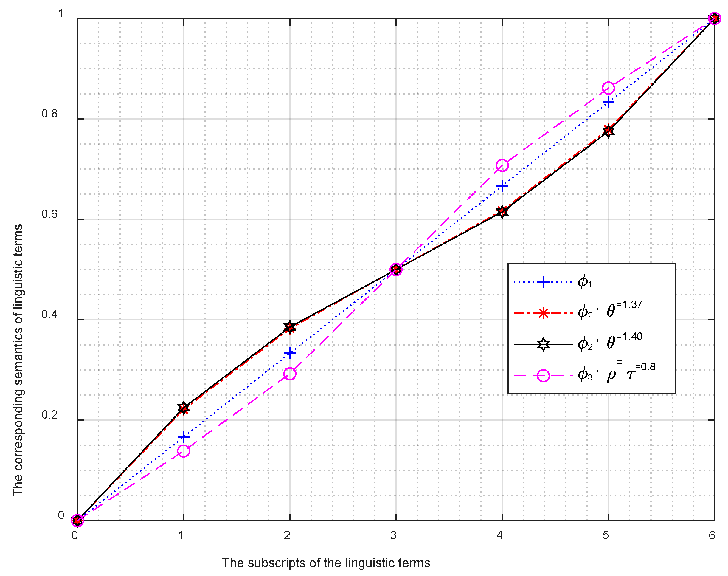
Let$\widehat{L}=\left\{\begin{array}{c}{\ell }_0=\mathrm{N}\left(\mathrm{none}\right),{\ell }_1=\mathrm{VL}\left(\mathrm{very} \mathrm{low}\right),{\ell }_2=\mathrm{L}\left(\mathrm{low}\right),{\ell }_3=\mathrm{M}\left(\mathrm{medium}\right), \\ {\ell }_4=\mathrm{H}\left( \mathrm{high} \right),{\ell }_5=\mathrm{VH}\left(\mathrm{very} \mathrm{high}\right),{\ell }_6=\mathrm{P}\left(\mathrm{perfect}\right)\end{array}\right\}$be a LTS with seven terms.Figure 1, Figure 2 and Figure 3 show the balanced distribution of$\widehat{L}$, unbalanced distribution of$\widehat{L}$in an increasing trend and the unbalanced distribution of$\widehat{L}$in a decreasing trend, respectively. Besides, Figure 4 represents the relationships between LTs of$\widehat{L}$and their corresponding semantics under different situations.

Figure 1. The uniformly distributed linguistic terms set.

Figure 2. The semantics of the unbalanced distributed LTS in ASG increasing trend.

Figure 3. The unbalanced distributed LTS in ASG decreasing trend.

Figure 4. The relationships between LTs and their corresponding semantics under different situations.

Meanwhile, to avoid an information loss and to facilitate the calculation process, the LSF $\phi$ can be further generalized to an extended continuous LTS as follows:

Definition 4 

([57]).Let${\widehat{L}}_{\left[0,2t\right]}=\left\{{\ell }_d|{\ell }_0\le {\ell }_d\le {\ell }_{2t},d\in \left[0,2t\right]\right\}$be an extended continuous LTS and${\kappa }_d\in \left[0,1\right]$be a real number, then the LSF${\phi }^{*}$is defined as

$${\phi }^{*}:{\widehat{L}}_{\left[0,2t\right]}\to {\kappa }_d$$

(5)

where${\phi }^{*}$is also a strictly monotonically increasing function, and its inverse is expressed as${\phi }^{*}{}^{-1}$.

Example 2.

Let${\widehat{L}}_{\left[0,6\right]}=\left\{{\ell }_d|d\in \left[0,6\right]\right\}$be a continuous LTS, then the inverse corresponding to the LSFs${\phi }_1^{\ast }$,${\phi }_2^{\ast }$and${\phi }_3^{\ast }$can be obtained as follows:

(1) If${\phi }_1^{\ast }\left({\ell }_d\right)={\kappa }_d=\frac{d}{6} \left(d=\left[0,6\right]\right)$, then${\phi }_1^{\ast }{}^{-1}\left({\kappa }_d\right)={\ell }_{6\times {\kappa }_d}\left({\kappa }_d\in \left[0,1\right]\right).$

(2) If${\phi }_2^{\ast }\left({\ell }_d\right)={\kappa }_d=\{\begin{array}{l}\frac{{\theta }^3-{\theta }^{3-d}}{2\left({\theta }^3-1\right)}, 0\le d\le 3\\ \frac{{\theta }^3+{\theta }^{d-3}-2}{2\left({\theta }^3-1\right)}, 3< d\le 6\end{array}$, then${\phi }_2^{\ast }{}^{-1}\left({\kappa }_d\right)=\{\begin{array}{l}{\ell }_{3-{\log }_{\theta }\left[{\theta }^3-\left(2{\theta }^3-2\right){\kappa }_d\right]}, {\kappa }_d\in \left[0,0.5\right],\\ {\ell }_{3+{\log }_{\theta }\left[\left(2{\theta }^3-2\right){\kappa }_d-{\theta }^3+2\right]},{\kappa }_d\in \left(0.5,1\right]. \end{array}$

(3) If${\phi }_3^{\ast }\left({\ell }_d\right)={\kappa }_d=\{\begin{array}{l}\frac{3^{\rho }-{\left(3-d\right)}^{\rho }}{2\times 3^{\rho }}, 0\le d\le 3\\ \frac{3^{\tau }+{\left(d-3\right)}^{\tau }}{2\times 3^{\tau }}, 3<d\le 6\end{array}$, then${\phi }_3^{\ast }{}^{-1}\left({\kappa }_d\right)=\{\begin{array}{l}{\ell }_{3-{\left[3^{\rho }-2\times 3^{\rho }\times {\kappa }_d\right]}^{1/\rho }},{\kappa }_d\in \left[0,0.5\right],\\ {\ell }_{3+{\left[2\times 3^{\tau }\times {\kappa }_d-3^{\tau }\right]}^{1/\tau }},{\kappa }_d\in \left(0.5,1\right]. \end{array}$

2.3. Fermatean Fuzzy Linguistic Set

Definition 5 

([41]).A FFS$\widehat{F}$in a fixed set$X=\left\{x_1,x_2,\dots ,x_n\right\}$is given by

$$\widehat{F}=\left\{⟨x_j,{\xi }_{\widehat{F}}\left(x_j\right),{\psi }_{\widehat{F}}\left(x_j\right)⟩|x_j\in X\right\}$$

(6)

where${\xi }_{\widehat{F}}\left(x_j\right)$and${\psi }_{\widehat{F}}\left(x_j\right)$denote, respectively, the DM and DNM of$x_j\in X$to the set$\widehat{F}$, with the conditions${\xi }_{\widehat{F}}:X\to \left[0,1\right]$,${\psi }_{\widehat{F}}:X\to \left[0,1\right]$and$0\le {\left({\xi }_{\widehat{F}}\left(x_j\right)\right)}^3+{\left({\psi }_{\widehat{F}}\left(x_j\right)\right)}^3\le 1 \forall x\in X$.

For all $x_j\in X$, the corresponding degree of hesitancy (DH) is defined as ${\zeta }_{\widehat{F}}\left(x_j\right)=\sqrt[3]{1-{\left({\xi }_{\widehat{F}}\left(x_j\right)\right)}^3-{\left({\psi }_{\widehat{F}}\left(x_j\right)\right)}^3}.$ In the interest of simplicity, Senapati and Yager [41] called the pair $⟨{\xi }_{\widehat{F}}\left(x_j\right),{\psi }_{\widehat{F}}\left(x_j\right)⟩$ a FFLN and denoted by $\alpha =⟨{\xi }_{\alpha },{\psi }_{\alpha }⟩,$ which satisfies the conditions ${\xi }_{\alpha }\in \left[0,1\right],{\psi }_{\alpha }\in \left[0,1\right]$ and $0\le {\left({\xi }_{\alpha }\right)}^3+{\left({\psi }_{\alpha }\right)}^3\le 1.$

Definition 6 

([53]).Let$X=\left\{x_1,x_2,\dots ,x_n\right\}$be a fixed set and${\widehat{L}}_{\left[0,2t\right]}=\left\{{\ell }_d|{\ell }_0\le {\ell }_d\le {\ell }_{2t},d\in \left[0,2t\right]\right\}$be an extended continuous LTS, then a FFLS can be defined as

$$F=\left\{⟨x_j,{\ell }_{{\sigma }_F\left(x_j\right)},{\xi }_F\left(x_j\right),{\psi }_F\left(x_j\right)⟩|x_j\in X\right\}$$

(7)

where${\ell }_{{\sigma }_F\left(x_j\right)}\in {\widehat{L}}_{\left[0,2t\right]}$, ${\xi }_F:X\to \left[0,1\right]$and${\psi }_F:X\to \left[0,1\right]$, satisfying$0\le {\left({\xi }_F\left(x_j\right)\right)}^3+{\left({\psi }_F\left(x_j\right)\right)}^3\le 1 \forall x_j\in X$. The numbers${\xi }_F\left(x_j\right)$and${\psi }_F\left(x_j\right)$represent, respectively, the DM and DNM of$x_j\in X$to the linguistic term${\ell }_{{\sigma }_F\left(x_j\right)}$. For all$x_j\in X$, if${\zeta }_F\left(x_j\right)=\sqrt[3]{1-{\left({\xi }_F\left(x_j\right)\right)}^3-{\left({\psi }_F\left(x_j\right)\right)}^3}$, then${\zeta }_F\left(x_j\right)$is called the DH of$x_j\in X$to${\ell }_{{\sigma }_F\left(x_j\right)}$.

Note that when ${\xi }_F\left(x_j\right)=1$ and ${\psi }_F\left(x_j\right)=0 \forall x_j\in X$, the FFLS reduces to the LTS. In particular, when $X$ has only one element, the FFLS is reduced into $⟨{\ell }_{{\sigma }_F\left(x\right)},{\xi }_F\left(x\right),{\psi }_F\left(x\right)⟩$. For convenience, the triplet $⟨{\ell }_{{\sigma }_F\left(x\right)},{\xi }_F\left(x\right),{\psi }_F\left(x\right)⟩$ is called a FFLN and simply denoted by $\wp =⟨{\ell }_{\sigma (\wp )},{\xi }_{\wp },{\psi }_{\wp }⟩$, which meets the conditions ${\xi }_{\wp }\in \left[0,1\right],{\psi }_{\wp }\in \left[0,1\right]$ and $0\le {\left({\xi }_{\wp }\right)}^3+{\left({\psi }_{\wp }\right)}^3\le 1.$ We indicate the collection of all FFLNs by $\Omega$.

Definition 7 

([54]).Let${\widehat{L}}_{\left[0,2t\right]}$be an extended continuous LTS,$\wp =⟨{\ell }_{\sigma (\wp )},{\xi }_{\wp },{\psi }_{\wp }⟩$, ${\wp }_1=⟨{\ell }_{\sigma \left({\wp }_1\right)},{\xi }_{{\wp }_1},{\psi }_{{\wp }_1}⟩$and${\wp }_2=⟨{\ell }_{\sigma \left({\wp }_2\right)},{\xi }_{{\wp }_2},{\psi }_{{\wp }_2}⟩$be any three FFLNs, where${\ell }_{\sigma (\wp )},{\ell }_{\sigma \left({\wp }_1\right)},{\ell }_{\sigma \left({\wp }_2\right)}\in {\widehat{L}}_{\left[0,2t\right]}$. Further, consider that${\phi }^{*}$and${\phi }^{*}{}^{-1}$denote a linguistic scale function and its inverse function, respectively. Then, by using the LSF, some algebraic operational laws on FFLNs were defined by Liu et al. [54] as follows:

(i). 

${\wp }_1\oplus {\wp }_2=⟨{\phi }^{*}{}^{-1}\left({\phi }^{*}\left({\ell }_{\sigma \left({\wp }_1\right)}\right)+{\phi }^{*}\left({\ell }_{\sigma \left({\wp }_2\right)}\right)\right),\sqrt[3]{{\xi }_{{\wp }_1}^3+{\xi }_{{\wp }_2}^3-{\xi }_{{\wp }_1}^3{\xi }_{{\wp }_2}^3},{\psi }_{{\wp }_1}{\psi }_{{\wp }_2}⟩;$

(ii). 

${\wp }_1\otimes {\wp }_2=⟨{\phi }^{*}{}^{-1}\left({\phi }^{*}\left({\ell }_{\sigma \left({\wp }_1\right)}\right){\phi }^{*}\left({\ell }_{\sigma \left({\wp }_2\right)}\right)\right),{\xi }_{{\wp }_1}{\xi }_{{\wp }_2},\sqrt[3]{{\psi }_{{\wp }_1}^3+{\psi }_{{\wp }_2}^3-{\psi }_{{\wp }_1}^3{\psi }_{{\wp }_2}^3}⟩;$

(iii). 

$\lambda \wp =⟨{\phi }^{*}{}^{-1}\left(\lambda {\phi }^{*}\left({\ell }_{\sigma (\wp )}\right)\right),\sqrt[3]{1-{\left(1-{\xi }_{\wp }^3\right)}^{\lambda }},{\left({\psi }_{\wp }\right)}^{\lambda }⟩, \lambda \ge 0;$

(iv). 

${\wp }^{\lambda }=⟨{\phi }^{*}{}^{-1}\left({\left({\phi }^{*}\left({\ell }_{\sigma (\wp )}\right)\right)}^{\lambda }\right),{\left({\xi }_{\wp }\right)}^{\lambda },\sqrt[3]{1-{\left(1-{\psi }_{\wp }^3\right)}^{\lambda }}⟩, \lambda \ge 0;$

(v). 

$neg(\wp )=⟨{\phi }^{*}{}^{-1}\left({\phi }^{*}\left({\ell }_{2t}\right)-{\phi }^{*}\left({\ell }_{\sigma (\wp )}\right)\right),{\psi }_{\wp },{\xi }_{\wp }⟩.$

Definition 8 

([54]).Let$\wp =⟨{\ell }_{\sigma (\wp )},{\xi }_{\wp },{\psi }_{\wp }⟩$be a FFLN and${\phi }^{*}$be a LSF, the score and accuracy functions of$\wp$are defined as

$$\mathfrak{S}(\wp )={\phi }^{*}\left({\ell }_{\sigma (\wp )}\right)\times \left(\frac{{\xi }_{\wp }^3+1-{\psi }_{\wp }^3}{2}\right) \mathrm{and} \mathfrak{A}(\wp )={\phi }^{*}\left({\ell }_{\sigma (\wp )}\right)\times \left({\xi }_{\wp }^3+{\psi }_{\wp }^3\right)$$

(8)

For any two FFLNs ${\wp }_1=⟨{\ell }_{\sigma \left({\wp }_1\right)},{\xi }_{{\wp }_1},{\psi }_{{\wp }_1}⟩$ and ${\wp }_2=⟨{\ell }_{\sigma \left({\wp }_2\right)},{\xi }_{{\wp }_2},{\psi }_{{\wp }_2}⟩$, the comparison rules between ${\wp }_1$ and ${\wp }_2$ are given as

(i).

If $\mathfrak{S}\left({\wp }_1\right)>\mathfrak{S}\left({\wp }_2\right), \mathrm{then} {\wp }_1\succ {\wp }_2;$

(ii).

If $\mathfrak{S}\left({\wp }_1\right)=\mathfrak{S}\left({\wp }_2\right),$ then: (a) $\mathfrak{A}\left({\wp }_1\right)>\mathfrak{A}\left({\wp }_2\right), \mathrm{then} {\wp }_1\succ {\wp }_2;$ (b) $\mathfrak{A}\left({\wp }_1\right)=\mathfrak{A}\left({\wp }_2\right), \mathrm{then} {\wp }_1={\wp }_2.$

Some shortcomings of the operational laws given in Definition 7

Here, we consider a numerical example in order to show the shortcomings of the operations on FFLNs defined by Liu et al. [54].

Example 3.

Let${\widehat{L}}_{\left[0,6\right]}=\left\{{\ell }_d|d\in \left[0,6\right]\right\}$be an extended continuous LTS,${\wp }_1=⟨{\ell }_3,0.3,0.6⟩$, ${\wp }_2=⟨{\ell }_5,0.5,0.7⟩$${\wp }_3=⟨{\ell }_1,0,0.5⟩$, ${\wp }_4=⟨{\ell }_3,0,0.7⟩$, ${\wp }_5=⟨{\ell }_4,0.8,0⟩$and${\wp }_6=⟨{\ell }_6,0.6,0⟩$be six FFLNs. If${\phi }^{*}\left({\ell }_{\sigma \left(a\right)}\right)={\phi }_2^{\ast }\left({\ell }_{\sigma \left(a\right)}\right)\left(\theta =1.4\right)$and$\lambda =4$, then according to the operational laws given in Definition 7, we have

(i). 

${\wp }_1\oplus {\wp }_2=⟨{\phi }_2^{\ast }{}^{-1}\left({\phi }_2^{\ast }\left({\ell }_3\right)+{\phi }_2^{\ast }\left({\ell }_5\right)\right),\sqrt[3]{{0.3}^3+{0.5}^3-{0.3}^3{0.5}^3},0.6\times 0.7⟩$

$=⟨{\phi }_2^{\ast }{}^{-1}\left(0.5000+0.7752\right),0.5279,0.4200⟩=⟨{\phi }_2^{\ast }{}^{-1}\left(1.2752\right),0.5279,0.4200⟩$.

Here, we see that ${\phi }_2^{\ast }\left({\ell }_3\right)+{\phi }_2^{\ast }\left({\ell }_5\right)=1.2752>1$, therefore, ${\phi }_2^{\ast }{}^{-1}\left({\phi }_2^{\ast }\left({\ell }_3\right)+{\phi }_2^{\ast }\left({\ell }_5\right)\right)={\phi }_2^{\ast }{}^{-1}\left(1.2752\right)$ is undefined.

(ii). 

${\wp }_1\otimes {\wp }_3=⟨{\phi }_2^{\ast }{}^{-1}\left({\phi }_2^{\ast }\left({\ell }_3\right){\phi }_2^{\ast }\left({\ell }_1\right)\right),0.3\times 0,\sqrt[3]{{0.6}^3+{0.5}^3-{0.6}^3\times {0.5}^3}⟩$

$$=⟨{\phi }_2^{\ast }{}^{-1}\left(0.5000\times 0.2248\right),0.0000,0.6797⟩=⟨{\ell }_{0.4619},0.0000,0.6797⟩$$

(9)

and

$$\begin{gathered} {\wp }_1\otimes {\wp }_4=⟨{\phi }_2^{\ast }{}^{-1}\left({\phi }_2^{\ast }\left({\ell }_3\right){\phi }_2^{\ast }\left({\ell }_3\right)\right),0.3\times 0,\sqrt[3]{{0.6}^3+{0.7}^3-{0.6}^3\times {0.7}^3}⟩ \\ =⟨{\phi }_2^{\ast }{}^{-1}\left(0.5000+0.5000\right),0.0000,0.7856⟩=⟨{\ell }_6,0.0000,0.7856⟩ \end{gathered}$$

(10)

From Equations (9) and (10), it is clear that there is no effect of nonmembership values on the membership values of${\wp }_1\otimes {\wp }_3$and${\wp }_1\otimes {\wp }_4$. In general, if${\wp }_1=⟨{\ell }_{\sigma \left({\wp }_1\right)},{\xi }_{{\wp }_1},{\psi }_{{\wp }_1}⟩$, ${\wp }_2=⟨{\ell }_{\sigma \left({\wp }_2\right)},{\xi }_{{\wp }_2},{\psi }_{{\wp }_2}⟩$and${\wp }_3=⟨{\ell }_{\sigma \left({\wp }_3\right)},{\xi }_{{\wp }_3},{\psi }_{{\wp }_3}⟩$are three different FFLNs satisfying,${\xi }_{{\wp }_2}={\xi }_{{\wp }_3}=0,{\psi }_{{\wp }_2}\ne {\psi }_{{\wp }_3}$then we always obtain${\xi }_{{\wp }_1\otimes {\wp }_2}={\xi }_{{\wp }_1\otimes {\wp }_3}=0.$This outcome does not match our intuition.

(iii). 

${\wp }_2\oplus {\wp }_5=⟨{\phi }_2^{\ast }{}^{-1}\left({\phi }_2^{\ast }\left({\ell }_5\right)+{\phi }_2^{\ast }\left({\ell }_4\right)\right),\sqrt[3]{{0.5}^3+{0.8}^3-{0.5}^3\times {0.8}^3},0.7\times 0,⟩$

$$=⟨{\phi }_2^{\ast }{}^{-1}\left(0.7752+0.6147\right),0.8306,0.0000⟩=⟨{\phi }_2^{\ast }{}^{-1}\left(1.3899\right),0.8306,0.0000⟩$$

(11)

and

$$\begin{gathered} {\wp }_2\oplus {\wp }_6=⟨{\phi }_2^{\ast }{}^{-1}\left({\phi }_2^{\ast }\left({\ell }_5\right)+{\phi }_2^{\ast }\left({\ell }_6\right)\right),\sqrt[3]{{0.5}^3+{0.6}^3-{0.5}^3\times {0.6}^3},0.7\times 0⟩ \\ =⟨{\phi }_2^{\ast }{}^{-1}\left(0.7752+1.0000\right),0.6797,0.0000⟩=⟨{\phi }_2^{\ast }{}^{-1}\left(1.7752\right),0.6797,0.0000⟩ \end{gathered}$$

(12)

The obtained resulting values in Equations (11) and (12) indicate that there is no effect of the membership values on the nonmembership values of${\wp }_2\oplus {\wp }_5$and${\wp }_2\oplus {\wp }_6$. In general, if${\wp }_1=⟨{\ell }_{\sigma \left({\wp }_1\right)},{\xi }_{{\wp }_1},{\psi }_{{\wp }_1}⟩$, ${\wp }_2=⟨{\ell }_{\sigma \left({\wp }_2\right)},{\xi }_{{\wp }_2},{\psi }_{{\wp }_2}⟩$and${\wp }_3=⟨{\ell }_{\sigma \left({\wp }_3\right)},{\xi }_{{\wp }_3},{\psi }_{{\wp }_3}⟩$are three different FFLNs satisfying,${\xi }_{{\wp }_2}\ne {\xi }_{{\wp }_3},{\psi }_{{\wp }_2}={\psi }_{{\wp }_3}=0$then we always obtain${\psi }_{{\wp }_1\oplus {\wp }_2}={\psi }_{{\wp }_1\oplus {\wp }_3}=0$. Additionally,${\phi }_2^{\ast }{}^{-1}\left(1.3899\right)$and${\phi }_2^{\ast }{}^{-1}\left(1.7752\right)$are undefined.

$$4{\wp }_1=⟨{\phi }_2^{\ast }{}^{-1}\left(4\times {\phi }_2^{\ast }\left({\ell }_3\right)\right),\sqrt[3]{1-{\left(1-{0.3}^3\right)}^4},{\left(0.6\right)}^4⟩=⟨{\phi }_2^{\ast }{}^{-1}\left(2.0000\right),0.4698,0.1296⟩,$$

(13)

$$4{\wp }_2=⟨{\phi }_2^{\ast }{}^{-1}\left(4\times {\phi }_2^{\ast }\left({\ell }_5\right)\right),\sqrt[3]{1-{\left(1-{0.5}^3\right)}^4},{\left(0.7\right)}^4⟩=⟨{\phi }_2^{\ast }{}^{-1}\left(3.1008\right),0.7452,0.2401⟩$$

(14)

From Equations (13) and (14), we can see that${\phi }_2^{\ast }{}^{-1}\left(2.0000\right)$and${\phi }_2^{\ast }{}^{-1}\left(3.1008\right)$are undefined because here${\kappa }_d>1$. Hence, $4{\wp }_1$and$4{\wp }_2$are not FFLNs.

Based on the above analysis, we conclude that the operational laws defined in Definition 7 are not suitable for FFLNs. Therefore, in order to nullify the above shortcomings, it is necessary to modify these operational laws. In the next section, we first define some new modified operational laws for FFLNs based on LSF and discuss their properties in detail. Then, we introduce some aggregation operators for aggregating different FFLNs.

3. Fermatean Fuzzy Aggregation Operators

3.1. Improved Operational Laws for FFLNs Based on LSF

Here, we define some improved operational laws for FFLNs, which overcome the shortcomings of the existing operations.

Definition 9.

Let${\widehat{L}}_{\left[0,2t\right]}$be an extended continuous LTS,$\wp =⟨{\ell }_{\sigma (\wp )},{\xi }_{\wp },{\psi }_{\wp }⟩$, ${\wp }_1=⟨{\ell }_{\sigma \left({\wp }_1\right)},{\xi }_{{\wp }_1},{\psi }_{{\wp }_1}⟩$and${\wp }_2=⟨s_{\sigma \left({\wp }_2\right)},{\xi }_{{\wp }_2},{\psi }_{{\wp }_2}⟩$be three FFLNs, where${\ell }_{\sigma (\wp )},{\ell }_{\sigma \left({\wp }_1\right)},{\ell }_{\sigma \left({\wp }_2\right)}\in {\widehat{L}}_{\left[0,2t\right]}$. Further, consider that${\phi }^{*}$ and ${\phi }^{*}{}^{-1}$ denote a linguistic scale function and its inverse function, respectively. The improved operational laws between them based on LSFs are defined as

(i) 

${\wp }_1\tilde{\oplus }{\wp }_2=⟨{\phi }^{*}{}^{-1}\left({\phi }^{*}\left({\ell }_{\sigma \left({\wp }_1\right)}\right)+{\phi }^{*}\left({\ell }_{\sigma \left({\wp }_2\right)}\right)-{\phi }^{*}\left({\ell }_{\sigma \left({\wp }_1\right)}\right){\phi }^{*}\left({\ell }_{\sigma \left({\wp }_2\right)}\right)\right),\sqrt[3]{{\xi }_{{\wp }_1}^3+{\xi }_{{\wp }_2}^3-{\xi }_{{\wp }_1}^3{\xi }_{{\wp }_2}^3}, \sqrt[3]{{\psi }_{{\wp }_1}^3+{\psi }_{{\wp }_2}^3-{\psi }_{{\wp }_1}^3{\psi }_{{\wp }_2}^3-{\psi }_{{\wp }_1}^3{\xi }_{{\wp }_2}^3-{\xi }_{{\wp }_1}^3{\psi }_{{\wp }_2}^3}⟩$

$=⟨{\phi }^{*}{}^{-1}\left(1-\left(1-{\phi }^{*}\left({\ell }_{\sigma \left({\wp }_1\right)}\right)\right)\left(1-{\phi }^{*}\left({\ell }_{\sigma \left({\wp }_2\right)}\right)\right)\right),\sqrt[3]{1-\left(1-{\xi }_{{\wp }_1}^3\right)\left(1-{\xi }_{{\wp }_2}^3\right)}, \sqrt[3]{\left(1-{\xi }_{{\wp }_1}^3\right)\left(1-{\xi }_{{\wp }_2}^3\right)-\left(1-\left({\xi }_{{\wp }_1}^3+{\psi }_{{\wp }_1}^3\right)\right)\left(1-\left({\xi }_{{\wp }_2}^3+{\psi }_{{\wp }_2}^3\right)\right)}⟩;$

(ii) 

${\wp }_1\tilde{\otimes }{\wp }_2=⟨{\phi }^{*}{}^{-1}\left({\phi }^{*}\left({\ell }_{\sigma \left({\wp }_1\right)}\right){\phi }^{*}\left({\ell }_{\sigma \left({\wp }_2\right)}\right)\right),\sqrt[3]{{\xi }_{{\wp }_1}^3+{\xi }_{{\wp }_2}^3-{\xi }_{{\wp }_1}^3{\xi }_{{\wp }_2}^3-{\xi }_{{\wp }_1}^3{\psi }_{{\wp }_2}^3-{\psi }_{{\wp }_1}^3{\xi }_{{\wp }_2}^3},\sqrt[3]{{\psi }_{{\wp }_1}^3+{\psi }_{{\wp }_2}^3-{\psi }_{{\wp }_1}^3{\psi }_{{\wp }_2}^3}⟩$$=⟨{\phi }^{*}{}^{-1}\left({\phi }^{*}\left({\ell }_{\sigma \left({\wp }_1\right)}\right){\phi }^{*}\left({\ell }_{\sigma \left({\wp }_2\right)}\right)\right),\sqrt[3]{\left(1-{\psi }_{{\wp }_1}^3\right)\left(1-{\psi }_{{\wp }_2}^3\right)-\left(1-\left({\xi }_{{\wp }_1}^3+{\psi }_{{\wp }_1}^3\right)\right)\left(1-\left({\xi }_{{\wp }_2}^3+{\psi }_{{\wp }_2}^3\right)\right)},\sqrt[3]{1-\left(1-{\psi }_{{\wp }_1}^3\right)\left(1-{\psi }_{{\wp }_2}^3\right)}⟩;$

(iii) 

$\lambda \tilde{\ast }\wp =⟨{\phi }^{*}{}^{-1}\left(1-{\left(1-{\phi }^{*}\left({\ell }_{\sigma (\wp )}\right)\right)}^{\lambda }\right),\sqrt[3]{1-{\left(1-{\xi }_{\wp }^3\right)}^{\lambda }},\sqrt[3]{{\left(1-{\xi }_{\wp }^3\right)}^{\lambda }-{\left(1-\left({\xi }_{\wp }^3+{\psi }_{\wp }^3\right)\right)}^{\lambda }}⟩, \lambda >0;$

(iv) 

$\wp \widetilde{^}\lambda =⟨{\phi }^{*}{}^{-1}\left({\left({\phi }^{*}\left({\ell }_{\sigma (\wp )}\right)\right)}^{\lambda }\right),\sqrt[3]{{\left(1-{\psi }_{\wp }^3\right)}^{\lambda }-{\left(1-\left({\xi }_{\wp }^3+{\psi }_{\wp }^3\right)\right)}^{\lambda }},\sqrt[3]{1-{\left(1-{\psi }_{\wp }^3\right)}^{\lambda }}⟩,\lambda >0.$

Theorem 1.

The numbers${\wp }_1\tilde{\oplus }{\wp }_2$, ${\wp }_1\tilde{\otimes }{\wp }_2$,$\lambda \tilde{\ast }\wp$, and$\wp \widetilde{^}\lambda$are also FFLNs.

Proof. 

Here, we shall prove only ${\wp }_1\tilde{\oplus }{\wp }_2$ and $\lambda \tilde{\ast }\wp$ are FFLNs, while others can be shown similarly. Since ${\wp }_i=⟨{\ell }_{\sigma \left({\wp }_i\right)},{\xi }_{{\wp }_i},{\psi }_{{\wp }_i}⟩\left(i=1,2\right)$ are two FFLNs, where ${\ell }_{\sigma \left({\wp }_i\right)}\in {\widehat{L}}_{\left[0,2t\right]}$, ${\xi }_{{\wp }_i},{\psi }_{{\wp }_i}\in \left[0,1\right]$ and $0\le {\xi }_{{\wp }_i}^3+{\psi }_{{\wp }_i}^3\le 1$, $i=1,2.$ For ${\ell }_{\sigma \left({\wp }_1\right)},{\ell }_{\sigma \left({\wp }_2\right)}\in {\widehat{L}}_{\left[0,2t\right]}$, based on the definition of the LSFs, we know $0\le {\phi }^{*}\left({\ell }_{\sigma \left({\wp }_1\right)}\right),{\phi }^{*}\left({\ell }_{\sigma \left({\wp }_2\right)}\right)\le 1$. Then, $0\le 1-\left(1-{\phi }^{*}\left({\ell }_{\sigma \left({\wp }_1\right)}\right)\right)\left(1-{\phi }^{*}\left({\ell }_{\sigma \left({\wp }_2\right)}\right)\right)\le 1$ $\Rightarrow {\phi }^{*}{}^{-1}\left(1-\left(1-{\phi }^{*}\left({\ell }_{\sigma \left({\wp }_1\right)}\right)\right)\left(1-{\phi }^{*}\left({\ell }_{\sigma \left({\wp }_2\right)}\right)\right)\right)\in {\widehat{L}}_{\left[0,2t\right]}.$ Now $0\le {\xi }_{{\wp }_1},{\xi }_{{\wp }_2}\le 1$, which implies $0\le \left(1-{\xi }_{{\wp }_1}^3\right)\left(1-{\xi }_{{\wp }_2}^3\right)\le 1\iff 0\le \sqrt[3]{1-\left(1-{\xi }_{{\wp }_1}^3\right)\left(1-{\xi }_{{\wp }_2}^3\right)}\le 1$. Moreover, because $1-{\xi }_{{\wp }_1}^3\ge 1-{\xi }_{{\wp }_1}^3-{\psi }_{{\wp }_1}^3$ and $1-{\xi }_{{\wp }_2}^3\ge 1-{\xi }_{{\wp }_2}^3-{\psi }_{{\wp }_2}^3$, then $0\le \sqrt[3]{\left(1-{\xi }_{{\wp }_1}^3\right)\left(1-{\xi }_{{\wp }_2}^3\right)-\left(1-\left({\xi }_{{\wp }_1}^3+{\psi }_{{\wp }_1}^3\right)\right)\left(1-\left({\xi }_{{\wp }_2}^3+{\psi }_{{\wp }_2}^3\right)\right)}\le 1$.

Further ${\left(\sqrt[3]{1-\left(\begin{array}{l}\left(1-{\xi }_{{\wp }_1}^3\right)\\ \left(1-{\xi }_{{\wp }_2}^3\right)\end{array}\right)}\right)}^3+{\left(\sqrt[3]{\left(\begin{array}{l}\left(1-{\xi }_{{\wp }_1}^3\right)\\ \left(1-{\xi }_{{\wp }_2}^3\right)\end{array}\right)-\left(\begin{array}{l}\left(1-\left({\xi }_{{\wp }_1}^3+{\psi }_{{\wp }_1}^3\right)\right)\\ \left(1-\left({\xi }_{{\wp }_2}^3+{\psi }_{{\wp }_2}^3\right)\right)\end{array}\right)}\right)}^3=1-\left(1-\left({\xi }_{{\wp }_1}^3+{\psi }_{{\wp }_1}^3\right)\right)\left(1-\left({\xi }_{{\wp }_2}^3+{\psi }_{{\wp }_2}^3\right)\right)\le 1.$ Thus, it shows that the $a_1\tilde{\oplus }{a}_2$ is a FFLN.

For any $\lambda >0$, $0\le 1-{\left(1-{\phi }^{*}\left({\ell }_{\sigma (\wp )}\right)\right)}^{\lambda }\le 1$, which gives ${\phi }^{*}{}^{-1}\left(1-{\left(1-{\phi }^{*}\left({\ell }_{\sigma (\wp )}\right)\right)}^{\lambda }\right)\in {\widehat{L}}_{\left[0,2t\right]}.$ Additionally, $0\le {\xi }_{{\wp }_1},{\xi }_{{\wp }_2},{\psi }_{{\wp }_1},{\psi }_{{\wp }_2}\le 1$, which implies $0\le \sqrt[3]{1-{\left(1-{\xi }_{\wp }^3\right)}^{\lambda }}\le 1$ and $0\le \sqrt[3]{{\left(1-{\xi }_{\wp }^3\right)}^{\lambda }-{\left(1-\left({\xi }_{\wp }^3+{\psi }_{\wp }^3\right)\right)}^{\lambda }}\le 1$.

Further ${\left(\sqrt[3]{1-{\left(1-{\xi }_{\wp }^3\right)}^{\lambda }}\right)}^3+{\left(\sqrt[3]{{\left(1-{\xi }_{\wp }^3\right)}^{\lambda }-{\left(1-\left({\xi }_{\wp }^3+{\psi }_{\wp }^3\right)\right)}^{\lambda }}\right)}^3=1-{\left(1-\left({\xi }_{\wp }^3+{\psi }_{\wp }^3\right)\right)}^{\lambda }\le 1.$ Hence, $\lambda \tilde{\ast }\wp$ is also a FFLN.

This completes the proof. □

Example 4.

Let${\widehat{L}}_{\left[0,6\right]}=\left\{{\ell }_d|d\in \left[0,6\right]\right\}$be an extended continuous LTS,$\wp =⟨{\ell }_2,0.4,0.5⟩$,${\wp }_1=⟨{\ell }_3,0.3,0.6⟩$,${\wp }_2=⟨{\ell }_5,0.5,0.7⟩$be three FFLNs and$\lambda =5$. Then, according to the modified operation laws, we obtained the following results as shown in Table 1:

Table 1. Values of different operations.

Operation	${\phi }^{*}={\phi }_1^{\ast }$	${\phi }^{*}={\phi }_2^{\ast } \mathrm{and} \theta =1.4$	${\phi }^{*}={\phi }_3^{\ast } \mathrm{and} \rho =\tau =0.8$
${\wp }_1\tilde{\oplus }{\wp }_2$	$⟨{\ell }_{5.4996},0.5297,0.7655⟩$	$⟨{\ell }_{5.5418},0.5297,0.7655⟩$	$⟨{\ell }_{5.4896},0.5297,0.7655⟩$
${\wp }_1\tilde{\otimes }{\wp }_2$	$⟨{\ell }_{2.5002},0.4826,0.7856⟩$	$⟨{\ell }_{2.0169},0.4826,0.7856⟩$	$⟨{\ell }_{2.7468},0.4826,0.7856⟩$
$\lambda \tilde{\ast }\wp$	$⟨{\ell }_{5.2098},0.6149,0.6945⟩$	$⟨{\ell }_{5.6483},0.6149,0.6945⟩$	$⟨{\ell }_{4.7348},0.6149,0.6945⟩$
$\wp \widetilde{^}\lambda$	$⟨{\ell }_{0.0246},0.5355,0.7452⟩$	$⟨{\ell }_{0.0323},0.5355,0.7452⟩$	$⟨{\ell }_{0.0157},0.5355,0.7452⟩$

Further, if we consider Example 3 again and utilize the improved operational laws summarized in Definition 9, Table 2 presents the obtained results.

Table 2. Calculation results of Example 3 based on the proposed operational laws.

Operation	${\phi }^{*}={\phi }_2^{\ast } \mathrm{and} \theta =1.4$
${\wp }_1\tilde{\oplus }{\wp }_2$	$⟨{\ell }_{5.5418},0.5279,0.7655⟩$
${\wp }_1\tilde{\otimes }{\wp }_3$	$⟨{\ell }_{0.4582},0.2869,0.6797⟩$
${\wp }_1\tilde{\otimes }{\wp }_4$	$⟨{\ell }_{1.1365},0.2608,0.7856⟩$
${\wp }_2\tilde{\oplus }{\wp }_5$	$⟨{\ell }_{5.6534},0.8306,0.5511⟩$
${\wp }_2\tilde{\oplus }{\wp }_6$	$⟨{\ell }_{6.0000},0.6797,0.6455⟩$
$4\tilde{\ast }{\wp }_1$	$⟨{\ell }_{5.7540},0.4698,0.8281⟩$
$4\tilde{\ast }{\wp }_2$	$⟨{\ell }_{5.9902},0.7452,0.7969⟩$

The obtained calculation results verify that the improved operational laws are more reasonable and realistic as per our intuition.

Theorem 2.

Let${\widehat{L}}_{\left[0,2t\right]}$be an extended continuous LTS, and${\wp }_1=⟨{\ell }_{\sigma \left({\wp }_1\right)},{\xi }_{{\wp }_1},{\psi }_{{\wp }_1}⟩$, ${\wp }_2=⟨{\ell }_{\sigma \left({\wp }_2\right)},{\xi }_{{\wp }_2},{\psi }_{{\wp }_2}⟩$and${\wp }_3=⟨{\ell }_{\sigma \left({\wp }_3\right)},{\xi }_{{\wp }_3},{\psi }_{{\wp }_3}⟩$be three FFLNs, where${\ell }_{\sigma \left({\wp }_1\right)},{\ell }_{\sigma \left({\wp }_2\right)},{\ell }_{\sigma \left({\wp }_3\right)}\in {\widehat{L}}_{\left[0,2t\right]}$. The following results hold:

(i). 

${\wp }_1\tilde{\oplus }{\wp }_2={\wp }_2\tilde{\oplus }{\wp }_1$;

(ii). 

${\wp }_1\tilde{\otimes }{\wp }_2={\wp }_2\tilde{\otimes }{\wp }_1$;

(iii). 

$\left({\wp }_1\tilde{\oplus }{\wp }_2\right)\tilde{\oplus }{\wp }_3={\wp }_1\tilde{\oplus }\left({\wp }_2\tilde{\oplus }{\wp }_3\right)$;

(iv). 

$\left({\wp }_1\tilde{\otimes }{\wp }_2\right)\tilde{\otimes }{\wp }_3={\wp }_1\tilde{\otimes }\left({\wp }_2\tilde{\otimes }{\wp }_3\right).$

Proof. 

The results follow directly from Definition 9, so we omit the proofs of them. □

Theorem 3. 

Let${\widehat{L}}_{\left[0,2t\right]}$be an extended continuous LTS,$\wp =⟨{\ell }_{\sigma (\wp )},{\xi }_{\wp },{\psi }_{\wp }⟩$${\wp }_1=⟨{\ell }_{\sigma \left({\wp }_1\right)},{\xi }_{{\wp }_1},{\psi }_{{\wp }_1}⟩$, and${\wp }_2=⟨{\ell }_{\sigma \left({\wp }_2\right)},{\xi }_{{\wp }_2},{\psi }_{{\wp }_2}⟩$be three FFLNs and$\lambda ,{\lambda }_1,{\lambda }_2>0$, where${\ell }_{\sigma (\wp )},{\ell }_{\sigma \left({\wp }_2\right)},{\ell }_{\sigma \left({\wp }_2\right)}\in {\widehat{L}}_{\left[0,2t\right]}$, then

(i). 

$\left(\lambda \tilde{\ast }{\wp }_1\right)\tilde{\oplus }\left(\lambda \tilde{\ast }{\wp }_2\right)=\lambda \tilde{\ast }\left({\wp }_1\tilde{\oplus }{\wp }_2\right)$;

(ii). 

$\left({\lambda }_1\tilde{\ast }\wp \right)\tilde{\oplus }\left({\lambda }_2\widehat{\ast }\wp \right)=\left({\lambda }_1+{\lambda }_2\right)\tilde{\ast }\wp$

(iii). 

$\left({\wp }_1\widetilde{^}\lambda \right)\tilde{\otimes }\left({\wp }_2\widetilde{^}\lambda \right)=\left({\wp }_1\tilde{\otimes }{\wp }_2\right)\widetilde{^}\lambda$;

(iv). 

$\left(\wp \widetilde{^}{\lambda }_1\right)\tilde{\otimes }\left(\wp \widetilde{^}{\lambda }_2\right)=\wp \widetilde{^}\left({\lambda }_1+{\lambda }_2\right)$;

(v). 

${\lambda }_1\tilde{\ast }\left({\lambda }_2\tilde{\ast }\wp \right)=\left({\lambda }_1{\lambda }_2\right)\tilde{\ast }\wp$;

(vi). 

$\left(\wp \widetilde{^}{\lambda }_1\right)\widetilde{^}{\lambda }_2=\wp \widetilde{^}\left({\lambda }_1{\lambda }_2\right)$.

(vii). 

$neg\left({\wp }_1\tilde{\oplus }{\wp }_2\right)=neg\left({\wp }_1\right)\tilde{\otimes }neg\left({\wp }_2\right)$

(viii). 

$neg\left({\wp }_1\tilde{\otimes }{\wp }_2\right)=neg\left({\wp }_1\right)\tilde{\oplus }neg\left({\wp }_2\right)$;

(ix). 

$\left(neg(\wp )\right)\widetilde{^}\lambda =neg\left(\lambda \tilde{\ast }\wp \right)$;

(x). 

$\lambda \tilde{\ast }\left(neg(\wp )\right)=neg\left(\wp \widetilde{^}\lambda \right)$.

Proof. 

Here, we only prove the parts (i), (iii), (v), (vii), and (ix); the others can be proved similarly.

(i) From Definition 9, we have

$$\lambda \tilde{\ast }{\wp }_1=⟨{\phi }^{*}{}^{-1}\left(1-{\left(1-{\phi }^{*}\left({\ell }_{\sigma \left({\wp }_1\right)}\right)\right)}^{\lambda }\right),\sqrt[3]{1-{\left(1-{\xi }_{{\wp }_1}^3\right)}^{\lambda }},\sqrt[3]{{\left(1-{\xi }_{{\wp }_1}^3\right)}^{\lambda }-{\left(1-\left({\xi }_{{\wp }_1}^3+{\psi }_{{\wp }_1}^3\right)\right)}^{\lambda }}⟩,$$

(15)

and

$$\lambda \tilde{\ast }{\wp }_2=⟨{\phi }^{*}{}^{-1}\left(1-{\left(1-{\phi }^{*}\left({\ell }_{\sigma \left({\wp }_2\right)}\right)\right)}^{\lambda }\right),\sqrt[3]{1-{\left(1-{\xi }_{{\wp }_2}^3\right)}^{\lambda }},\sqrt[3]{{\left(1-{\xi }_{{\wp }_2}^3\right)}^{\lambda }-{\left(1-\left({\xi }_{{\wp }_2}^3+{\psi }_{{\wp }_2}^3\right)\right)}^{\lambda }}⟩,$$

(16)

Using Equations (15) and (16), we obtain

$$\begin{gathered} \left(\lambda \tilde{\ast }{\wp }_1\right)\tilde{\oplus }\left(\lambda \tilde{\ast }{\wp }_2\right) \\ =⟨\begin{array}{l}{\phi }^{*}{}^{-1}\left(\begin{array}{l}1-\left(1-{\phi }^{*}\left({\phi }^{*}{}^{-1}\left(1-{\left(1-{\phi }^{*}\left({\ell }_{\sigma \left({\wp }_1\right)}\right)\right)}^{\lambda }\right)\right)\right)\\ \left(1-{\phi }^{*}\left({\phi }^{*}{}^{-1}\left(1-{\left(1-{\phi }^{*}\left({\ell }_{\sigma \left({\wp }_2\right)}\right)\right)}^{\lambda }\right)\right)\right)\end{array}\right),\sqrt[3]{1-\left(1-{\left(\sqrt[3]{1-{\left(1-{\xi }_{{\wp }_1}^3\right)}^{\lambda }}\right)}^3\right)\left(1-{\left(\sqrt[3]{1-{\left(1-{\xi }_{{\wp }_1}^3\right)}^{\lambda }}\right)}^3\right)},\\ \sqrt[3]{\begin{array}{l}\left(1-{\left(\sqrt[3]{1-{\left(1-{\xi }_{{\wp }_1}^3\right)}^{\lambda }}\right)}^3\right)\left(1-{\left(\sqrt[3]{1-{\left(1-{\xi }_{{\wp }_2}^3\right)}^{\lambda }}\right)}^3\right) \\ \hfill -\left(1-\left({\left(\sqrt[3]{1-{\left(1-{\xi }_{{\wp }_1}^3\right)}^{\lambda }}\right)}^3+{\left(\sqrt[3]{{\left(1-{\xi }_{{\wp }_1}^3\right)}^{\lambda }-{\left(1-\left({\xi }_{{\wp }_1}^3+{\psi }_{{\wp }_1}^3\right)\right)}^{\lambda }}\right)}^3\right)\right) \hfill \\ \left(1-\left({\left(\sqrt[3]{1-{\left(1-{\xi }_{{\wp }_2}^3\right)}^{\lambda }}\right)}^3+{\left(\sqrt[3]{{\left(1-{\xi }_{{\wp }_2}^3\right)}^{\lambda }-{\left(1-\left({\xi }_{{\wp }_2}^3+{\psi }_{{\wp }_2}^3\right)\right)}^{\lambda }}\right)}^3\right)\right)\end{array}}\end{array}⟩ \\ =⟨\begin{array}{c}{\phi }^{*}{}^{-1}\left(1-{\left(\left(1-{\phi }^{*}\left({\ell }_{\sigma \left({\wp }_1\right)}\right)\right)\left(1-{\phi }^{*}\left({\ell }_{\sigma \left({\wp }_2\right)}\right)\right)\right)}^{\lambda }\right),\sqrt[3]{1-{\left(\left(1-{\xi }_{{\wp }_1}^3\right)\left(1-{\xi }_{{\wp }_2}^3\right)\right)}^{\lambda }}, \\ \sqrt[3]{{\left(\left(1-{\xi }_{{\wp }_1}^3\right)\left(1-{\xi }_{{\wp }_2}^3\right)\right)}^{\lambda }-{\left(\left(1-\left({\xi }_{{\wp }_1}^3+{\psi }_{{\wp }_1}^3\right)\right)\left(1-\left({\xi }_{{\wp }_2}^3+{\psi }_{{\wp }_2}^3\right)\right)\right)}^{\lambda }}\end{array}⟩=\lambda \tilde{\ast }\left({\wp }_1\tilde{\oplus }{\wp }_2\right). \end{gathered}$$

(iii) According to Definition 9, we have

$${\wp }_1\widetilde{^}\lambda =⟨{\phi }^{*}{}^{-1}\left({\left({\phi }^{*}\left({\ell }_{\sigma \left({\wp }_1\right)}\right)\right)}^{\lambda }\right),\sqrt[3]{{\left(1-{\psi }_{{\wp }_1}^3\right)}^{\lambda }-{\left(1-\left({\xi }_{{\wp }_1}^3+{\psi }_{{\wp }_1}^3\right)\right)}^{\lambda }},\sqrt[3]{1-{\left(1-{\psi }_{{\wp }_1}^3\right)}^{\lambda }}⟩,$$

(17)

and

$${\wp }_2\widetilde{^}\lambda =⟨{\phi }^{*}{}^{-1}\left({\left({\phi }^{*}\left({\ell }_{\sigma \left({\wp }_2\right)}\right)\right)}^{\lambda }\right),\sqrt[3]{{\left(1-{\psi }_{{\wp }_2}^3\right)}^{\lambda }-{\left(1-\left({\xi }_{{\wp }_2}^3+{\psi }_{{\wp }_2}^3\right)\right)}^{\lambda }},\sqrt[3]{1-{\left(1-{\psi }_{{\wp }_2}^3\right)}^{\lambda }}⟩.$$

(18)

By Equations (17) and (18), we obtain

$$\begin{gathered} \left({\wp }_1\widetilde{^}\lambda \right)\tilde{\otimes }\left({\wp }_2\widetilde{^}\lambda \right)=⟨\begin{array}{c}{\phi }^{*}{}^{-1}\left({\phi }^{*}\left({\phi }^{*}{}^{-1}\left({\left({\phi }^{*}\left({\ell }_{\sigma \left({\wp }_1\right)}\right)\right)}^{\lambda }\right)\right){\phi }^{*}\left({\phi }^{*}{}^{-1}\left({\left({\phi }^{*}\left({\ell }_{\sigma \left({\wp }_2\right)}\right)\right)}^{\lambda }\right)\right)\right),\\ \sqrt[3]{\left(\begin{array}{l}\left(1-{\left(\sqrt[3]{1-{\left(1-{\psi }_{{\wp }_1}^3\right)}^{\lambda }}\right)}^3\right)\\ \left(1-{\left(\sqrt[3]{1-{\left(1-{\psi }_{{\wp }_2}^3\right)}^{\lambda }}\right)}^3\right)\end{array}\right)-\left(\begin{array}{l}\left(1-\left(\begin{array}{l}{\left(\sqrt[3]{{\left(1-{\psi }_{{\wp }_1}^3\right)}^{\lambda }-{\left(1-\left({\xi }_{{\wp }_1}^3+{\psi }_{{\wp }_1}^3\right)\right)}^{\lambda }}\right)}^3\\ +{\left(\sqrt[3]{1-{\left(1-{\psi }_{{\wp }_1}^3\right)}^{\lambda }}\right)}^3\end{array}\right)\right)\\ \left(1-\left(\begin{array}{l}{\left(\sqrt[3]{{\left(1-{\psi }_{{\wp }_2}^3\right)}^{\lambda }-{\left(1-\left({\xi }_{{\wp }_2}^3+{\psi }_{{\wp }_2}^3\right)\right)}^{\lambda }}\right)}^3\\ +{\left(\sqrt[3]{1-{\left(1-{\psi }_{{\wp }_2}^3\right)}^{\lambda }}\right)}^3\end{array}\right)\right)\end{array}\right)} ,\\ \sqrt[3]{1-\left(1-{\left(\sqrt[3]{1-{\left(1-{\psi }_{{\wp }_1}^3\right)}^{\lambda }}\right)}^3\right)\left(1-{\left(\sqrt[3]{1-{\left(1-{\psi }_{{\wp }_2}^3\right)}^{\lambda }}\right)}^3\right)} \end{array}⟩ \\ =⟨\begin{array}{c}{\phi }^{*}{}^{-1}\left({\left({\phi }^{*}\left({\ell }_{\sigma \left({\wp }_1\right)}\right){\phi }^{*}\left({\ell }_{\sigma \left({\wp }_2\right)}\right)\right)}^{\lambda }\right),\sqrt[3]{{\left(\left(1-{\psi }_{{\wp }_1}^3\right)\left(1-{\psi }_{{\wp }_2}^3\right)\right)}^{\lambda }-{\left(\left(1-\left({\xi }_{{\wp }_1}^3+{\psi }_{{\wp }_1}^3\right)\right)\left(1-\left({\xi }_{{\wp }_2}^3+{\psi }_{{\wp }_2}^3\right)\right)\right)}^{\lambda }} ,\\ \sqrt[3]{1-{\left(\left(1-{\psi }_{{\wp }_1}^3\right)\left(1-{\psi }_{{\wp }_2}^3\right)\right)}^{\lambda }}\end{array}⟩=\left({\wp }_1\tilde{\otimes }{\wp }_2\right)\widetilde{^}\lambda . \end{gathered}$$

(v) For two positive real numbers ${\lambda }_1$ and ${\lambda }_2$, we have

$$\begin{gathered} {\lambda }_1\tilde{\ast }\left({\lambda }_2\tilde{\ast }\wp \right)={\lambda }_1\left(⟨{\phi }^{*}{}^{-1}\left(1-{\left(1-{\phi }^{*}\left({\ell }_{\sigma (\wp )}\right)\right)}^{{\lambda }_2}\right),\sqrt[3]{1-{\left(1-{\xi }_{\wp }^3\right)}^{{\lambda }_2}},\sqrt[3]{{\left(1-{\xi }_{\wp }^3\right)}^{{\lambda }_2}-{\left(1-\left({\xi }_{\wp }^3+{\psi }_{\wp }^3\right)\right)}^{{\lambda }_2}}⟩\right), \\ =⟨\begin{array}{l}{\phi }^{*}{}^{-1}\left(1-{\left(1-{\phi }^{*}\left({\phi }^{*}{}^{-1}\left(1-{\left(1-{\phi }^{*}\left({\ell }_{\sigma (\wp )}\right)\right)}^{{\lambda }_2}\right)\right)\right)}^{{\lambda }_1}\right),\sqrt[3]{1-{\left(1-{\left(\sqrt[3]{1-{\left(1-{\xi }_{\wp }^3\right)}^{{\lambda }_2}}\right)}^3\right)}^{{\lambda }_1}},\\ \sqrt[3]{{\left(1-{\left(\sqrt[3]{1-{\left(1-{\xi }_{\wp }^3\right)}^{{\lambda }_2}}\right)}^3\right)}^{{\lambda }_1}-{\left(1-\left({\left(\sqrt[3]{1-{\left(1-{\xi }_{\wp }^3\right)}^{{\lambda }_2}}\right)}^3+{\left(\sqrt[3]{{\left(1-{\xi }_{\wp }^3\right)}^{{\lambda }_2}-{\left(1-\left({\xi }_{\wp }^3+{\psi }_{\wp }^3\right)\right)}^{{\lambda }_2}}\right)}^3\right)\right)}^{{\lambda }_1}}\end{array}⟩ \\ =⟨{\phi }^{*}{}^{-1}\left(1-{\left(1-{\phi }^{*}\left({\ell }_{\sigma (\wp )}\right)\right)}^{{\lambda }_1{\lambda }_2}\right),\sqrt[3]{1-{\left(1-{\xi }_{\wp }^3\right)}^{{\lambda }_1{\lambda }_2}},\sqrt[3]{{\left(1-{\xi }_{\wp }^3\right)}^{{\lambda }_1{\lambda }_2}-{\left(1-\left({\xi }_{\wp }^3+{\psi }_{\wp }^3\right)\right)}^{{\lambda }_1{\lambda }_2}}⟩ \\ =\left({\lambda }_1{\lambda }_2\right)\tilde{\ast }\wp \end{gathered}$$

(vii) From Definitions 7 and 9, we have

$$\begin{gathered} neg\left({\wp }_1\tilde{\oplus }{\wp }_2\right)=⟨\begin{array}{c}{\phi }^{*}{}^{-1}\left({\phi }^{*}\left({\ell }_{2t}\right)-{\phi }^{*}\left({\phi }^{*}{}^{-1}\left(1-\left(1-{\phi }^{*}\left({\ell }_{\sigma \left({\wp }_1\right)}\right)\right)\left(1-{\phi }^{*}\left({\ell }_{\sigma \left({\wp }_2\right)}\right)\right)\right)\right)\right),\\ \sqrt[3]{\left(1-{\xi }_{{\wp }_1}^3\right)\left(1-{\xi }_{{\wp }_2}^3\right)-\left(1-\left({\xi }_{{\wp }_1}^3+{\psi }_{{\wp }_1}^3\right)\right)\left(1-\left({\xi }_{{\wp }_2}^3+{\psi }_{{\wp }_2}^3\right)\right)},\sqrt[3]{1-\left(1-{\xi }_{{\wp }_1}^3\right)\left(1-{\xi }_{{\wp }_2}^3\right)}\end{array}⟩ \\ =⟨\begin{array}{c}{\phi }^{*}{}^{-1}\left({\phi }^{*}\left({\ell }_{2t}\right)-\left(1-\left(1-{\phi }^{*}\left({\ell }_{\sigma \left({\wp }_1\right)}\right)\right)\left(1-{\phi }^{*}\left({\ell }_{\sigma \left({\wp }_2\right)}\right)\right)\right)\right),\\ \sqrt[3]{\left(1-{\xi }_{{\wp }_1}^3\right)\left(1-{\xi }_{{\wp }_2}^3\right)-\left(1-\left({\xi }_{{\wp }_1}^3+{\psi }_{{\wp }_1}^3\right)\right)\left(1-\left({\xi }_{{\wp }_2}^3+{\psi }_{{\wp }_2}^3\right)\right)},\sqrt[3]{1-\left(1-{\xi }_{{\wp }_1}^3\right)\left(1-{\xi }_{{\wp }_2}^3\right)}\end{array}⟩ \\ =⟨\begin{array}{l}{\phi }^{*}{}^{-1}\left(\left({\phi }^{*}\left({\ell }_{2t}\right)-{\phi }^{*}\left({\ell }_{\sigma \left({\wp }_1\right)}\right)\right)\left({\phi }^{*}\left({\ell }_{2t}\right)-{\phi }^{*}\left({\ell }_{\sigma \left({\wp }_2\right)}\right)\right)\right),\\ \sqrt[3]{\left(1-{\xi }_{{\wp }_1}^3\right)\left(1-{\xi }_{{\wp }_2}^3\right)-\left(1-\left({\psi }_{{\wp }_1}^3+{\xi }_{{\wp }_1}^3\right)\right)\left(1-\left({\psi }_{{\wp }_2}^3+{\xi }_{{\wp }_2}^3\right)\right)},\sqrt[3]{1-\left(1-{\xi }_{{\wp }_1}^3\right)\left(1-{\xi }_{{\wp }_2}^3\right)}\end{array}⟩; \\ =neg\left({\wp }_1\right)\tilde{\otimes }neg\left({\wp }_2\right) \end{gathered}$$

(ix) $\left(neg(\wp )\right)\widetilde{^}\lambda ={\left(⟨{\phi }^{*}{}^{-1}\left({\phi }^{*}\left({\ell }_{2t}\right)-{\phi }^{*}\left({\ell }_{\sigma (\wp )}\right)\right),{\psi }_{\wp },{\xi }_{\wp }⟩\right)}^{\lambda }$

$$\begin{gathered} =⟨{\phi }^{*}{}^{-1}\left({\left({\phi }^{*}\left({\ell }_{2t}\right)-{\phi }^{*}\left({\ell }_{\sigma (\wp )}\right)\right)}^{\lambda }\right),\sqrt[3]{{\left(1-{\xi }_{\wp }^3\right)}^{\lambda }-{\left(1-\left({\xi }_{\wp }^3+{\psi }_{\wp }^3\right)\right)}^{\lambda }},\sqrt[3]{1-{\left(1-{\xi }_{\wp }^3\right)}^{\lambda }}⟩ \\ =⟨{\phi }^{*}{}^{-1}\left({\phi }^{*}\left({\ell }_{2t}\right)-{\phi }^{*}\left({\phi }^{*}{}^{-1}\left(1-{\left(1-{\phi }^{*}\left({\ell }_{\sigma (\wp )}\right)\right)}^{\lambda }\right)\right)\right),\sqrt[3]{{\left(1-{\xi }_{\wp }^3\right)}^{\lambda }-{\left(1-\left({\xi }_{\wp }^3+{\psi }_{\wp }^3\right)\right)}^{\lambda }},\sqrt[3]{1-{\left(1-{\xi }_{\wp }^3\right)}^{\lambda }}⟩ \\ =neg\left(⟨{\phi }^{*}{}^{-1}\left(1-{\left(1-{\phi }^{*}\left({\ell }_{\sigma (\wp )}\right)\right)}^{\lambda }\right),\sqrt[3]{1-{\left(1-{\xi }_{\wp }^3\right)}^{\lambda }},\sqrt[3]{{\left(1-{\xi }_{\wp }^3\right)}^{\lambda }-{\left(1-\left({\xi }_{\wp }^3+{\psi }_{\wp }^3\right)\right)}^{\lambda }}⟩\right) \\ =neg\left(\lambda \tilde{\ast }\wp \right). \end{gathered}$$

This completes the proof. □

Next, by utilizing proposed improved operational laws on FFLNs, we propose some arithmetic and geometric aggregation operators for fusing a collection of FFLNs ${\wp }_i=⟨{\ell }_{\sigma \left({\wp }_i\right)},{\xi }_{{\wp }_i},{\psi }_{{\wp }_i}⟩\left(i=1,2,\dots ,n\right).$

3.2. FFL-Weighted Average (FFLWA) Operator

The weighted average (WA) is the most commonly used mean operator in a wide range of application areas. Here, we extend the idea of WA to the Fermetean fuzzy linguistic information environment and propose the following formal definition.

Definition 10.

Let${\wp }_i=⟨{\ell }_{\sigma \left({\wp }_i\right)},{\xi }_{{\wp }_i},{\psi }_{{\wp }_i}⟩\left(i=1,2,\dots ,n\right)$be a collection of FFLNs. The FFL-weighted average (FFLWA) operator is a mapping$\mathrm{FFLWA}:{\Omega }^n\to \Omega$, such that

$$\mathrm{FFLWA}\left({\wp }_1,{\wp }_2,\dots ,{\wp }_n\right)=\underset{i=1}{\overset{n}{\tilde{\oplus }}}\left(w_i\tilde{\ast }{\wp }_i\right),$$

(19)

where$w={\left(w_1,w_2,\dots ,w_n\right)}^T$is the weight vector of${\wp }_i$with$w_i\in \left[0,1\right]$, ${\displaystyle \sum _{i=1}^n{w}_i}=1.$Especially when$w={\left(\frac{1}{n},\frac{1}{n},\dots ,\frac{1}{n}\right)}^T$, the$\mathrm{FFLWA}$operator reduces to FFL-average (FFLA) operator, which is defined as

$$\mathrm{FFLWA}\left({\wp }_1,{\wp }_2,\dots ,{\wp }_n\right)=\frac{1}{n}\tilde{\ast }\left(\underset{i=1}{\overset{n}{\tilde{\oplus }}}{\wp }_i\right).$$

(20)

Theorem 4.

Let${\wp }_i=⟨{\ell }_{\sigma \left({\wp }_i\right)},{\xi }_{{\wp }_i},{\psi }_{{\wp }_i}⟩\left(i=1,2,\dots ,n\right)$be a collection of$n$FFLNs and$w={\left(w_1,w_2,\dots ,w_n\right)}^T$be the weight vector of${\wp }_i$with$w_i\in \left[0,1\right]$, ${\displaystyle \sum _{i=1}^n{w}_i}=1,$then the aggregated value by using the FFLWA operator is also a FFLN and

$$\mathrm{FFLWA}\left({\wp }_1,{\wp }_2,\dots ,{\wp }_n\right)=⟨\begin{array}{c}{\phi }^{*}{}^{-1}\left(1-{\displaystyle \prod _{i=1}^n{\left(1-{\phi }^{*}\left({\ell }_{\sigma \left({\wp }_i\right)}\right)\right)}^{w_i}}\right),\sqrt[3]{1-{\displaystyle \prod _{i=1}^n{\left(1-{\xi }_{{\wp }_i}^3\right)}^{w_i}}}, \\ \sqrt[3]{{\displaystyle \prod _{i=1}^n{\left(1-{\xi }_{{\wp }_i}^3\right)}^{w_i}}-{\displaystyle \prod _{i=1}^n{\left(1-\left({\xi }_{{\wp }_i}^3+{\psi }_{{\wp }_i}^3\right)\right)}^{w_i}}}\end{array}⟩.$$

(21)

Proof. 

The first result directly holds from Theorem 1. Using the principle of mathematical induction, we shall prove the result stated in Equation (21). Firstly, for $n=2$, by Definition 9, we obtain

$$\begin{array}{l}{w}_1\tilde{\ast }{\wp }_1=⟨{\phi }^{*}{}^{-1}\left(1-{\left(1-{\phi }^{*}\left({\ell }_{\sigma \left({\wp }_1\right)}\right)\right)}^{w_1}\right),\sqrt[3]{1-{\left(1-{\xi }_{{\wp }_1}^3\right)}^{w_1}},\sqrt[3]{{\left(1-{\xi }_{{\wp }_1}^3\right)}^{w_1}-{\left(1-\left({\xi }_{{\wp }_1}^3+{\psi }_{{\wp }_1}^3\right)\right)}^{w_1}}⟩,\\ w_2\tilde{\ast }{\wp }_2=⟨{\phi }^{*}{}^{-1}\left(1-{\left(1-{\phi }^{*}\left({\ell }_{\sigma \left({\wp }_2\right)}\right)\right)}^{w_2}\right),\sqrt[3]{1-{\left(1-{\xi }_{{\wp }_2}^3\right)}^{w_2}},\sqrt[3]{{\left(1-{\xi }_{{\wp }_2}^3\right)}^{w_2}-{\left(1-\left({\xi }_{{\wp }_2}^3+{\psi }_{{\wp }_2}^3\right)\right)}^{w_2}}⟩\end{array}\}.$$

(22)

Hence,

$$\mathrm{FFLWA}\left({\wp }_1,{\wp }_2\right)=⟨\begin{array}{c}{\phi }^{*}{}^{-1}\left(1-{\displaystyle \prod _{i=1}^2{\left(1-{\phi }^{*}\left({\ell }_{\sigma \left({\wp }_i\right)}\right)\right)}^{w_i}}\right),\sqrt[3]{1-{\displaystyle \prod _{i=1}^2{\left(1-{\xi }_{{\wp }_i}^3\right)}^{w_i}}}, \\ \sqrt[3]{{\displaystyle \prod _{i=1}^2{\left(1-{\xi }_{{\wp }_i}^3\right)}^{w_i}}-{\displaystyle \prod _{i=1}^2{\left(1-\left({\xi }_{{\wp }_i}^3+{\psi }_{{\wp }_i}^3\right)\right)}^{w_i}}}\end{array}⟩$$

(23)

Hence, the result is valid for $n=2$.

Next, assume that Equation (21) is true for $n=k$, i.e.,

$$\mathrm{FFLWA}\left({\wp }_1,{\wp }_2,\dots ,{\wp }_k\right)=⟨\begin{array}{c}{\phi }^{*}{}^{-1}\left(1-{\displaystyle \prod _{i=1}^k{\left(1-{\phi }^{*}\left({\ell }_{\sigma \left({\wp }_i\right)}\right)\right)}^{w_i}}\right),\sqrt[3]{1-{\displaystyle \prod _{i=1}^k{\left(1-{\xi }_{{\wp }_i}^3\right)}^{w_i}}}, \\ \sqrt[3]{{\displaystyle \prod _{i=1}^k{\left(1-{\xi }_{{\wp }_i}^3\right)}^{w_i}}-{\displaystyle \prod _{i=1}^k{\left(1-\left({\xi }_{{\wp }_i}^3+{\psi }_{{\wp }_i}^3\right)\right)}^{w_i}}}\end{array}⟩.$$

(24)

Then, for $n=k+1$, by Definition 10, we have

$$\begin{gathered} \mathrm{FFLWA}\left({\wp }_1,{\wp }_2,\dots ,{\wp }_k,{\wp }_{k+1}\right)=\mathrm{FFLWA}\left({\wp }_1,{\wp }_2,\dots ,{\wp }_k\right)\tilde{\oplus }\left(w_{k+1}\tilde{\ast }{\wp }_{k+1}\right) \\ =⟨\begin{array}{c}{\phi }^{*}{}^{-1}\left(1-{\displaystyle \prod _{i=1}^k{\left(1-{\phi }^{*}\left({\ell }_{\sigma \left({\wp }_i\right)}\right)\right)}^{w_i}}\right),\sqrt[3]{1-{\displaystyle \prod _{i=1}^k{\left(1-{\xi }_{{\wp }_i}^3\right)}^{w_i}}}, \\ \sqrt[3]{{\displaystyle \prod _{i=1}^k{\left(1-{\xi }_{{\wp }_i}^3\right)}^{w_i}}-{\displaystyle \prod _{i=1}^k{\left(1-\left({\xi }_{{\wp }_i}^3+{\psi }_{{\wp }_i}^3\right)\right)}^{w_i}}}\end{array}⟩\hspace{0.17em}\tilde{\oplus }⟨{\ell }_{\sigma \left({\wp }_{k+1}\right)},{\xi }_{{\wp }_{k+1}},{\psi }_{{\wp }_{k+1}}⟩ \\ =⟨\begin{array}{c}{\phi }^{*}{}^{-1}\left(1-{\displaystyle \prod _{i=1}^k{\left(1-{\phi }^{*}\left({\ell }_{\sigma \left({\wp }_i\right)}\right)\right)}^{w_i}{\left(1-{\phi }^{*}\left({\ell }_{\sigma \left({\wp }_{k+i}\right)}\right)\right)}^{w_{k+i}}}\right),\sqrt[3]{1-{\displaystyle \prod _{i=1}^k{\left(1-{\xi }_{{\wp }_i}^3\right)}^{w_i}{\left(1-{\xi }_{{\wp }_{k+1}}^3\right)}^{w_{k+1}}}}, \\ \sqrt[3]{{\displaystyle \prod _{i=1}^k{\left(1-{\xi }_{{\wp }_i}^3\right)}^{w_i}{\left(1-{\xi }_{{\wp }_{k+1}}^3\right)}^{w_{k+1}}}-{\displaystyle \prod _{i=1}^k{\left(1-\left({\xi }_{{\wp }_i}^3+{\psi }_{{\wp }_i}^3\right)\right)}^{w_i}{\left(1-\left({\xi }_{{\wp }_{k+1}}^3+{\psi }_{{\wp }_{k+1}}^3\right)\right)}^{w_{k+1}}}}\end{array}⟩ \\ =⟨\begin{array}{c}\hfill {\phi }^{*}{}^{-1}\left(1-{\displaystyle \prod _{i=1}^{k+1}{\left(1-{\phi }^{*}\left({\ell }_{\sigma \left(a_i\right)}\right)\right)}^{w_i}}\right),\sqrt[3]{1-{\displaystyle \prod _{i=1}^{k+1}{\left(1-{\xi }_{{\wp }_i}^3\right)}^{w_i}}}, \\ \sqrt[3]{{\displaystyle \prod _{i=1}^{k+1}{\left(1-{\xi }_{{\wp }_i}^3\right)}^{w_i}}-{\displaystyle \prod _{i=1}^{k+1}{\left(1-\left({\xi }_{{\wp }_i}^3+{\psi }_{{\wp }_i}^3\right)\right)}^{w_i}}}\end{array}⟩ \end{gathered}$$

(25)

i.e., the Equation (21) holds for $n=k+1$.

This proves the theorem. □

Theorem 5. 

The FFLWA operator, defined in Equation (21), holds the following properties:

(P1) (Idempotency): If${\wp }_i=\wp =⟨{\ell }_{\sigma (\wp )},{\xi }_{\wp },{\psi }_{\wp }⟩\hspace{0.17em}\hspace{0.17em}\hspace{0.17em}\forall \hspace{0.17em}i$, then

$$\mathrm{FFLWA}\left({\wp }_1,{\wp }_2,\dots ,{\wp }_n\right)=\wp .$$

(26)

(P2) (Monotonicity): Let${\wp }_i=⟨{\ell }_{\sigma \left({\wp }_i\right)},{\xi }_{{\wp }_i},{\psi }_{{\wp }_i}⟩$and${\aleph }_i=⟨{\ell }_{\sigma \left({\aleph }_i\right)},{\xi }_{{\aleph }_i},{\psi }_{{\aleph }_i}⟩\left(i=1,2,\dots ,n\right)$be two collections of FFLNs such that${\ell }_{\sigma \left({\wp }_i\right)}\le \hspace{0.17em}{\ell }_{\sigma \left({\aleph }_i\right)},{\xi }_{{\wp }_i}^3\le {\xi }_{{\aleph }_i}^3,{\xi }_{{\wp }_i}^3+{\psi }_{{\wp }_i}^3\ge {\xi }_{{\aleph }_i}^3+{\psi }_{{\aleph }_i}^3\forall i$, then

$$\mathrm{FFLWA}\left({\wp }_1,{\wp }_2,\dots ,{\wp }_n\right)\le \mathrm{FFLWA}\left({\aleph }_1,{\aleph }_2,\dots ,{\aleph }_n\right).$$

(27)

(P3) (Boundedness): Let

$${\wp }^{-}=⟨\begin{array}{l}\min \left({\ell }_{\sigma \left({\wp }_1\right)},{\ell }_{\sigma \left({\wp }_2\right)},\dots ,{\ell }_{\sigma \left({\wp }_n\right)}\right),\min \left({\xi }_{{\wp }_1}^3,{\xi }_{{\wp }_2}^3,\dots ,{\xi }_{{\wp }_n}^3\right),\max \left\{0,\left(\begin{array}{c}\max \left({\xi }_{{\wp }_1}^3+{\psi }_{{\wp }_1}^3,{\xi }_{{\wp }_2}^3+{\psi }_{{\wp }_2}^3,\dots ,{\xi }_{{\wp }_n}^3+{\psi }_{{\wp }_n}^3\right) \\ -\min \left({\xi }_{{\wp }_1}^3,{\xi }_{{\wp }_2}^3,\dots ,{\xi }_{{\wp }_n}^3\right)\end{array}\right)\right\}\\ \end{array}⟩,$$

and

$${\wp }^{+}=⟨\begin{array}{l}\max \left({\ell }_{\sigma \left({\wp }_1\right)},{\ell }_{\sigma \left({\wp }_2\right)},\dots ,{\ell }_{\sigma \left({\wp }_n\right)}\right),\max \left({\xi }_{{\wp }_1}^3,{\xi }_{{\wp }_2}^3,\dots ,{\xi }_{{\wp }_n}^3\right),\left(\begin{array}{c}\min \left({\xi }_{{\wp }_1}^3+{\psi }_{{\wp }_1}^3,{\xi }_{{\wp }_2}^3+{\psi }_{{\wp }_2}^3,\dots ,{\xi }_{{\wp }_n}^3+{\psi }_{{\wp }_n}^3\right) \\ -\max \left({\xi }_{{\wp }_1}^3,{\xi }_{{\wp }_2}^3,\dots ,{\xi }_{{\wp }_n}^3\right)\end{array}\right)\\ \end{array}⟩,$$

then

$${\wp }^{-}\le \mathrm{FFLWA}\left({\wp }_1,{\wp }_2,\dots ,{\wp }_n\right)\le {\wp }^{+}.$$

(P4): If$\aleph =⟨s_{\sigma (\aleph )},{\xi }_{\aleph },{\psi }_{\aleph }⟩$is another FFLN, then

$$\mathrm{FFLWA}\left({\wp }_1\tilde{\oplus }\aleph ,{\wp }_2\tilde{\oplus }\aleph ,\dots ,{\wp }_n\tilde{\oplus }\aleph \right)=\mathrm{FFLWA}\left({\wp }_1,{\wp }_2,\dots ,{\wp }_n\right)\tilde{\oplus }\aleph .$$

(28)

(P5): Let$\vartheta >0$be a real number, then

$$\mathrm{FFLWA}\left(\vartheta \tilde{\ast }{\wp }_1,\vartheta \tilde{\ast }{\wp }_2,\dots ,\vartheta \tilde{\ast }{\wp }_n\right)=\vartheta \tilde{\ast }\left(\mathrm{FFLWA}\left({\wp }_1,{\wp }_2,\dots ,{\wp }_n\right)\right).$$

(29)

(P6): Let$\aleph =⟨s_{\sigma (\aleph )},{\xi }_{\aleph },{\psi }_{\aleph }⟩$be another FFLN and$\vartheta >0$be a real number, then

$$\mathrm{FFLWA}\left(\left(\vartheta \tilde{\ast }{\wp }_1\right)\tilde{\oplus }\aleph ,\left(\vartheta \tilde{\ast }{\wp }_2\right)\tilde{\oplus }\aleph ,\dots ,\left(\vartheta \tilde{\ast }{\wp }_n\right)\tilde{\oplus }\aleph \right)=\left(\vartheta \tilde{\ast }\left(\mathrm{FFLWA}\left({\wp }_1,{\wp }_2,\dots ,{\wp }_n\right)\right)\right)\tilde{\oplus }b.$$

(30)

(P7): Let${\wp }_i=⟨{\ell }_{\sigma \left({\wp }_i\right)},{\xi }_{{\wp }_i},{\psi }_{{\wp }_i}⟩$and${\aleph }_i=⟨s_{\sigma \left({\aleph }_i\right)},{\xi }_{{\aleph }_i},{\psi }_{{\aleph }_i}⟩, \left(i=1,2,\dots ,n\right)$be two collections of FFLNs, then

$$\mathrm{FFLWA}\left({\wp }_1\tilde{\oplus }{\aleph }_1,{\wp }_2\tilde{\oplus }{\aleph }_2,\dots ,{\wp }_n\tilde{\oplus }{\aleph }_n\right)=\mathrm{FFLWA}\left({\wp }_1,{\wp }_2,\dots ,{\wp }_n\right)\tilde{\oplus }\mathrm{FFLWA}\left({\aleph }_1,{\aleph }_2,\dots ,{\aleph }_n\right).$$

(31)

Proof. 

(P1) Assume that ${\wp }_i=\wp =⟨{\ell }_{\sigma (\wp )},{\xi }_{\wp },{\psi }_{\wp }⟩\hspace{0.17em}\hspace{0.17em}\hspace{0.17em}\forall \hspace{0.17em}i$, then

$$\begin{gathered} \mathrm{FFLWA}\left({\wp }_1,{\wp }_2,\dots ,{\wp }_n\right)=\mathrm{FFLWA}\left(\wp ,\wp ,\dots ,\wp \right) \\ =⟨\begin{array}{c}{\phi }^{*}{}^{-1}\left(1-{\displaystyle \prod _{i=1}^n{\left(1-{\phi }^{*}\left({\ell }_{\sigma (\wp )}\right)\right)}^{w_i}}\right),\sqrt[3]{1-{\displaystyle \prod _{i=1}^n{\left(1-{\xi }_{\wp }^3\right)}^{w_i}}}, \hfill \\ \sqrt[3]{{\displaystyle \prod _{i=1}^n{\left(1-{\xi }_{\wp }^3\right)}^{w_i}}-{\displaystyle \prod _{i=1}^n{\left(1-\left({\xi }_{\wp }^3+{\psi }_{\wp }^3\right)\right)}^{w_i}}}\end{array}⟩ \\ =⟨\begin{array}{c}{\phi }^{*}{}^{-1}\left(1-{\left(1-{\phi }^{*}\left({\ell }_{\sigma (\wp )}\right)\right)}^{w_1+w_2+\cdots +w_n}\right),\sqrt[3]{1-{\left(1-{\xi }_{\wp }^3\right)}^{w_1+w_2+\cdots +w_n}}, \\ \sqrt[3]{{\left(1-{\xi }_{\wp }^3\right)}^{w_1+w_2+\cdots +w_n}-{\left(1-\left({\xi }_{\wp }^3+{\psi }_{\wp }^3\right)\right)}^{w_1+w_2+\cdots +w_n}}\end{array}⟩ \\ =⟨{\ell }_{\sigma (\wp )},{\xi }_{\wp },{\psi }_{\wp }⟩=\wp . \end{gathered}$$

(P2) Since ${\ell }_{\sigma \left({\wp }_i\right)}\le \hspace{0.17em}{\ell }_{\sigma \left({\aleph }_i\right)}$ and ${\phi }^{*}$ is a strictly monotonically increasing function, then

$$\begin{array}{c}{\ell }_{\sigma \left({\wp }_i\right)}\le \hspace{0.17em}{\ell }_{\sigma \left({\aleph }_i\right)}\iff 1-{\phi }^{*}\left({\ell }_{\sigma \left({\wp }_i\right)}\right)\ge 1-{\phi }^{*}\left({\ell }_{\sigma \left({\aleph }_i\right)}\right) \\ \iff {\phi }^{*}{}^{-1}\left(1-{\displaystyle \prod _{i=1}^n{\left(1-{\phi }^{*}\left({\ell }_{\sigma \left({\wp }_i\right)}\right)\right)}^{w_i}}\right)\le {\phi }^{*}{}^{-1}\left(1-{\displaystyle \prod _{i=1}^n{\left(1-{\phi }^{*}\left({\ell }_{\sigma \left({\aleph }_i\right)}\right)\right)}^{w_i}}\right)\end{array}\}.$$

(32)

As ${\xi }_{{\wp }_i}^3\le {\xi }_{{\aleph }_i}^3\left(i=1,2,\dots ,n\right) \mathrm{and} {\xi }_{{\wp }_i}^3+{\psi }_{{\wp }_i}^3\ge {\xi }_{{\aleph }_i}^3+{\psi }_{{\aleph }_i}^3\left(i=1,2,\dots ,n\right)$, we have

$$\begin{array}{c}\sqrt[3]{1-{\displaystyle \prod _{i=1}^n{\left(1-{\xi }_{{\wp }_i}^3\right)}^{w_i}}}\le \sqrt[3]{1-{\displaystyle \prod _{i=1}^n{\left(1-{\xi }_{{\aleph }_i}^3\right)}^{w_i}}}\\ \sqrt[3]{{\displaystyle \prod _{i=1}^n{\left(1-{\xi }_{{\wp }_i}^3\right)}^{w_i}}-{\displaystyle \prod _{i=1}^n{\left(1-\left({\xi }_{{\wp }_i}^3+{\psi }_{{\wp }_i}^3\right)\right)}^{w_i}}}\ge \sqrt[3]{{\displaystyle \prod _{i=1}^n{\left(1-{\xi }_{{\aleph }_i}^3\right)}^{w_i}}-{\displaystyle \prod _{i=1}^n{\left(1-\left({\xi }_{{\aleph }_i}^3+{\psi }_{{\aleph }_i}^3\right)\right)}^{w_i}}}\end{array}\}.$$

(33)

According to Definition 10, we have

$$\mathrm{FFLWA}\left({\wp }_1,{\wp }_2,\dots ,{\wp }_n\right)=⟨\begin{array}{c}{\phi }^{*}{}^{-1}\left(1-{\displaystyle \prod _{i=1}^n{\left(1-{\phi }^{*}\left({\ell }_{\sigma \left({\wp }_i\right)}\right)\right)}^{w_i}}\right),\sqrt[3]{1-{\displaystyle \prod _{i=1}^n{\left(1-{\xi }_{{\wp }_i}^3\right)}^{w_i}}}, \\ \sqrt[3]{{\displaystyle \prod _{i=1}^n{\left(1-{\xi }_{{\wp }_i}^3\right)}^{w_i}}-{\displaystyle \prod _{i=1}^n{\left(1-\left({\xi }_{{\wp }_i}^3+{\psi }_{{\wp }_i}^3\right)\right)}^{w_i}}}\end{array}⟩,$$

and

$$\mathrm{FFLWA}\left({\aleph }_1,{\aleph }_2,\dots ,{\aleph }_n\right)=⟨\begin{array}{c}{\phi }^{*}{}^{-1}\left(1-{\displaystyle \prod _{i=1}^n{\left(1-{\phi }^{*}\left({\ell }_{\sigma \left({\aleph }_i\right)}\right)\right)}^{w_i}}\right),\sqrt[3]{1-{\displaystyle \prod _{i=1}^n{\left(1-{\xi }_{{\aleph }_i}^3\right)}^{w_i}}}, \\ \sqrt[3]{{\displaystyle \prod _{i=1}^n{\left(1-{\xi }_{{\aleph }_i}^3\right)}^{w_i}}-{\displaystyle \prod _{i=1}^n{\left(1-\left({\xi }_{{\aleph }_i}^3+{\psi }_{{\aleph }_i}^3\right)\right)}^{w_i}}}\end{array}⟩$$

Now, using Definition 8, we obtain $\mathfrak{S}\left(\mathrm{FFLWA}\left({\wp }_1,{\wp }_2,\dots ,{\wp }_n\right)\right)\le \mathfrak{S}\left(\mathrm{FFLWA}\left({\aleph }_1,{\aleph }_2,\dots ,{\aleph }_n\right)\right)$, which gives

$$\mathrm{FFLWA}\left({\wp }_1,{\wp }_2,\dots ,{\wp }_n\right)\le \mathrm{FFLWA}\left({\aleph }_1,{\aleph }_2,\dots ,{\aleph }_n\right).$$

(P3) It directly follows from Property 2.

(P4) Since, so

$${\wp }_i\tilde{\oplus }\aleph =⟨\begin{array}{c}{\phi }^{*}{}^{-1}\left(1-\left(1-{\phi }^{*}\left({\ell }_{\sigma \left({\wp }_i\right)}\right)\right)\left(1-{\phi }^{*}\left({\ell }_{\sigma (\aleph )}\right)\right)\right),\sqrt[3]{1-\left(1-{\xi }_{{\wp }_i}^3\right)\left(1-{\xi }_{\aleph }^3\right)}, \hspace{1em}\\ \sqrt[3]{\left(1-{\xi }_{{\wp }_i}^3\right)\left(1-{\xi }_{\aleph }^3\right)-\left(1-\left({\xi }_{{\wp }_i}^3+{\psi }_{{\wp }_i}^3\right)\right)\left(1-\left({\xi }_{\aleph }^3+{\psi }_{\aleph }^3\right)\right)}\end{array}⟩$$

(34)

Therefore,

$$\begin{gathered} \mathrm{FFLWA}\left({\wp }_1\tilde{\oplus }\aleph ,{\wp }_2\tilde{\oplus }\aleph ,\dots ,{\wp }_n\tilde{\oplus }\aleph \right) \\ =⟨\begin{array}{r}{\phi }^{*}{}^{-1}\left(1-{\displaystyle \prod _{i=1}^n{\left(\left(1-{\phi }^{*}\left({\ell }_{\sigma \left({\wp }_i\right)}\right)\right)\left(1-{\phi }^{*}\left({\ell }_{\sigma (\aleph )}\right)\right)\right)}^{w_i}}\right),\sqrt[3]{1-{\displaystyle \prod _{i=1}^n{\left(\left(1-{\xi }_{{\wp }_i}^3\right)\left(1-{\xi }_{\aleph }^3\right)\right)}^{w_i}}}, \hspace{1em}\\ \sqrt[3]{{\displaystyle \prod _{i=1}^n{\left(\left(1-{\xi }_{{\wp }_i}^3\right)\left(1-{\xi }_{\aleph }^3\right)\right)}^{w_i}}-{\displaystyle \prod _{i=1}^n{\left(\left(1-\left({\xi }_{{\wp }_i}^3+{\psi }_{{\wp }_i}^3\right)\right)\left(1-\left({\xi }_{\aleph }^3+{\psi }_{\aleph }^3\right)\right)\right)}^{w_i}}}\end{array}⟩ \\ =⟨\begin{array}{r}{\phi }^{*}{}^{-1}\left(1-\left({\displaystyle \prod _{i=1}^n{\left(\left(1-{\phi }^{*}\left({\ell }_{\sigma \left({\wp }_i\right)}\right)\right)\right)}^{w_i}}\right)\left(1-{\phi }^{*}\left({\ell }_{\sigma (\aleph )}\right)\right)\right),\sqrt[3]{1-\left({\displaystyle \prod _{i=1}^n{\left(1-{\xi }_{{\wp }_i}^3\right)}^{w_i}}\right)\left(1-{\xi }_{\aleph }^3\right)}, \\ \sqrt[3]{\left({\displaystyle \prod _{i=1}^n{\left(1-{\xi }_{{\wp }_i}^3\right)}^{w_i}}\right)\left(1-{\xi }_{\aleph }^3\right)-\left({\displaystyle \prod _{i=1}^n{\left(1-\left({\xi }_{{\wp }_i}^3+{\psi }_{{\wp }_i}^3\right)\right)}^{w_i}}\right)\left(1-\left({\xi }_{\aleph }^3+{\psi }_{\aleph }^3\right)\right)}\end{array}⟩ \\ =⟨\begin{array}{c}{\phi }^{*}{}^{-1}\left(1-{\displaystyle \prod _{i=1}^n{\left(1-{\phi }^{*}\left({\ell }_{\sigma \left({\wp }_i\right)}\right)\right)}^{w_i}}\right),\sqrt[3]{1-{\displaystyle \prod _{i=1}^n{\left(1-{\xi }_{{\wp }_i}^3\right)}^{w_i}}}, \\ \sqrt[3]{{\displaystyle \prod _{i=1}^n{\left(1-{\xi }_{{\wp }_i}^3\right)}^{w_i}}-{\displaystyle \prod _{i=1}^n{\left(1-\left({\xi }_{{\wp }_i}^3+{\psi }_{{\wp }_i}^3\right)\right)}^{w_i}}}\end{array}⟩\tilde{\oplus }⟨{\ell }_{\sigma (\aleph )},{\xi }_{\aleph },{\psi }_{\aleph }⟩ \\ =\mathrm{FFLWA}\left({\wp }_1,{\wp }_2,\dots ,{\wp }_n\right)\tilde{\oplus }\aleph . \end{gathered}$$

(P5) For any $\vartheta >0$, we have

$$\vartheta \tilde{\ast }{\wp }_i=⟨{\phi }^{*}{}^{-1}\left(1-{\left(1-{\phi }^{*}\left({\ell }_{\sigma \left({\wp }_i\right)}\right)\right)}^{\vartheta }\right),\sqrt[3]{1-{\left(1-{\xi }_{{\wp }_i}^3\right)}^{\vartheta }},\sqrt[3]{{\left(1-{\xi }_{{\wp }_i}^3\right)}^{\vartheta }-{\left(1-\left({\xi }_{{\wp }_i}^3+{\psi }_{{\wp }_i}^3\right)\right)}^{\vartheta }}⟩.$$

(35)

Therefore,

$$\begin{array}{l}\mathrm{FFLWA}\left(\vartheta \tilde{\ast }{\wp }_1,\vartheta \tilde{\ast }{\wp }_2,\dots ,\vartheta \tilde{\ast }{\wp }_n\right)=⟨\begin{array}{c}{\phi }^{*}{}^{-1}\left(1-{\displaystyle \prod _{i=1}^n{\left({\left(1-{\phi }^{*}\left({\ell }_{\sigma \left({\wp }_i\right)}\right)\right)}^{\vartheta }\right)}^{w_i}}\right),\sqrt[3]{1-{\displaystyle \prod _{i=1}^n{\left({\left(1-{\xi }_{{\wp }_i}^3\right)}^{\vartheta }\right)}^{w_i}}}, \\ \sqrt[3]{{\displaystyle \prod _{i=1}^n{\left({\left(1-{\xi }_{{\wp }_i}^3\right)}^{\vartheta }\right)}^{w_i}}-{\displaystyle \prod _{i=1}^n{\left({\left(1-\left({\xi }_{{\wp }_i}^3+{\psi }_{{\wp }_i}^3\right)\right)}^{\vartheta }\right)}^{w_i}}}\end{array}⟩\\ =⟨\begin{array}{c}{\phi }^{*}{}^{-1}\left(1-{\displaystyle \prod _{i=1}^n{\left({\left(1-{\phi }^{*}\left({\ell }_{\sigma \left({\wp }_i\right)}\right)\right)}^{w_i}\right)}^{\vartheta }}\right),\sqrt[3]{1-{\displaystyle \prod _{i=1}^n{\left({\left(1-{\xi }_{{\wp }_i}^3\right)}^{w_i}\right)}^{\vartheta }}}, \\ \sqrt[3]{{\displaystyle \prod _{i=1}^n{\left({\left(1-{\xi }_{{\wp }_i}^3\right)}^{w_i}\right)}^{\vartheta }}-{\displaystyle \prod _{i=1}^n{\left({\left(1-\left({\xi }_{{\wp }_i}^3+{\psi }_{{\wp }_i}^3\right)\right)}^{w_i}\right)}^{\vartheta }}}\end{array}⟩\\ =\vartheta \tilde{\ast }\left(\mathrm{FFLWA}\left({\wp }_1,{\wp }_2,\dots ,{\wp }_n\right)\right).\end{array}$$

(P6) From Property 4, we know

$$\mathrm{FFLWA}\left({\wp }_1\tilde{\oplus }\aleph ,{\wp }_2\tilde{\oplus }\aleph ,\dots ,{\wp }_n\tilde{\oplus }\aleph \right)=\mathrm{FFLWA}\left({\wp }_1,{\wp }_2,\dots ,{\wp }_n\right)\tilde{\oplus }\aleph ,$$

(36)

and according to Property 5, we have

$$\mathrm{FFLWA}\left(\vartheta \tilde{\ast }{\wp }_1,\vartheta \tilde{\ast }{\wp }_2,\dots ,\vartheta \tilde{\ast }{\wp }_n\right)=\vartheta \tilde{\ast }\left(\mathrm{FFLWA}\left({\wp }_1,{\wp }_2,\dots ,{\wp }_n\right)\right).,$$

(37)

From Equations (36) and (37), we obtain the desired results.

(P7) Since ${\wp }_i,{\aleph }_i\in \Omega$, then

$${\wp }_i\tilde{\oplus }{\aleph }_i=⟨\begin{array}{c}{\phi }^{*}{}^{-1}\left(1-\left(1-{\phi }^{*}\left({\ell }_{\sigma \left({\wp }_i\right)}\right)\right)\left(1-{\phi }^{*}\left({\ell }_{\sigma \left({\aleph }_i\right)}\right)\right)\right),\sqrt[3]{1-\left(1-{\xi }_{{\wp }_i}^3\right)\left(1-{\xi }_{{\aleph }_i}^3\right)}, \hspace{1em}\\ \sqrt[3]{\left(1-{\xi }_{{\wp }_i}^3\right)\left(1-{\xi }_{{\aleph }_i}^3\right)-\left(1-\left({\xi }_{{\wp }_i}^3+{\psi }_{{\aleph }_i}^3\right)\right)\left(1-\left({\xi }_{{\wp }_i}^3+{\psi }_{{\aleph }_i}^3\right)\right)}\end{array}⟩.$$

(38)

Therefore,

$$\begin{array}{l}\mathrm{FFLWA}\left({\wp }_1\tilde{\oplus }{\aleph }_1,{\wp }_2\tilde{\oplus }{\aleph }_2,\dots ,{\wp }_n\tilde{\oplus }{\aleph }_n\right)\\ =⟨\begin{array}{c}{\phi }^{*}{}^{-1}\left(1-{\displaystyle \prod _{i=1}^n{\left(\left(1-{\phi }^{*}\left({\ell }_{\sigma \left({\wp }_i\right)}\right)\right)\left(1-{\phi }^{*}\left({\ell }_{\sigma \left({\aleph }_i\right)}\right)\right)\right)}^{w_i}}\right),\sqrt[3]{1-{\displaystyle \prod _{i=1}^n{\left(\left(1-{\xi }_{{\wp }_i}^3\right)\left(1-{\xi }_{{\aleph }_i}^3\right)\right)}^{w_i}}}, \\ \sqrt[3]{{\displaystyle \prod _{i=1}^n{\left(\left(1-{\xi }_{{\wp }_i}^3\right)\left(1-{\xi }_{{\aleph }_i}^3\right)\right)}^{w_i}}-{\displaystyle \prod _{i=1}^n{\left(\left(1-\left({\xi }_{{\wp }_i}^3+{\psi }_{{\aleph }_i}^3\right)\right)\left(1-\left({\xi }_{{\wp }_i}^3+{\psi }_{{\aleph }_i}^3\right)\right)\right)}^{w_i}}}\end{array}⟩\\ =⟨\begin{array}{c}{\phi }^{*}{}^{-1}\left(1-{\displaystyle \prod _{i=1}^n{\left(1-{\phi }^{*}\left({\ell }_{\sigma \left({\wp }_i\right)}\right)\right)}^{w_i}{\displaystyle \prod _{i=1}^n{\left(1-{\phi }^{*}\left({\ell }_{\sigma \left({\aleph }_i\right)}\right)\right)}^{w_i}}}\right),\sqrt[3]{1-{\displaystyle \prod _{i=1}^n{\left(1-{\xi }_{{\wp }_i}^3\right)}^{w_i}{\displaystyle \prod _{i=1}^n{\left(1-{\xi }_{{\aleph }_i}^3\right)}^{w_i}}}}, \\ \sqrt[3]{{\displaystyle \prod _{i=1}^n{\left(1-{\xi }_{{\wp }_i}^3\right)}^{w_i}{\displaystyle \prod _{i=1}^n{\left(1-{\xi }_{{\aleph }_i}^3\right)}^{w_i}}}-{\displaystyle \prod _{i=1}^n{\left(1-\left({\xi }_{{\wp }_i}^3+{\psi }_{{\wp }_i}^3\right)\right)}^{w_i}{\displaystyle \prod _{i=1}^n{\left(1-\left({\xi }_{{\aleph }_i}^3+{\psi }_{{\aleph }_i}^3\right)\right)}^{w_i}}}}\end{array}⟩\\ =⟨\begin{array}{c}{\phi }^{*}{}^{-1}\left(1-{\displaystyle \prod _{i=1}^n{\left(1-{\phi }^{*}\left({\ell }_{\sigma \left({\rho }_i\right)}\right)\right)}^{w_i}}\right),\sqrt[3]{1-{\displaystyle \prod _{i=1}^n{\left(1-{\xi }_{{\wp }_i}^3\right)}^{w_i}}}, \\ \sqrt[3]{{\displaystyle \prod _{i=1}^n{\left(1-{\xi }_{{\wp }_i}^3\right)}^{w_i}}-{\displaystyle \prod _{i=1}^n{\left(1-\left({\xi }_{{\wp }_i}^3+{\psi }_{{\wp }_i}^3\right)\right)}^{w_i}}}\end{array}⟩\tilde{\oplus }⟨\begin{array}{c}{\phi }^{*}{}^{-1}\left(1-{\displaystyle \prod _{i=1}^n{\left(1-{\phi }^{*}\left({\ell }_{\sigma \left({\wp }_i\right)}\right)\right)}^{w_i}}\right),\sqrt[3]{1-{\displaystyle \prod _{i=1}^n{\left(1-{\xi }_{{\wp }_i}^3\right)}^{w_i}}}, \\ \sqrt[3]{{\displaystyle \prod _{i=1}^n{\left(1-{\xi }_{{\wp }_i}^3\right)}^{w_i}}-{\displaystyle \prod _{i=1}^n{\left(1-\left({\xi }_{{\wp }_i}^3+{\psi }_{{\wp }_i}^3\right)\right)}^{w_i}}}\end{array}⟩\\ =\mathrm{FFLWA}\left({\wp }_1,{\wp }_2,\dots ,{\wp }_n\right)\tilde{\oplus }\mathrm{FFLWA}\left({\aleph }_1,{\aleph }_2,\dots ,{\aleph }_n\right).\end{array}$$

This proves the theorem. □

3.3. FFL-Ordered Weighted Average (FFLOWA) Operator

The ordered weighted averaging (OWA) operator [59] is an aggregation operator that provides a parameterized family of aggregation operators between the minimum and the maximum. In this subsection, we extend the idea of the FFLWA operator into the FFLOWA operator based on the OWA operator.

Definition 11.Let${\wp }_i=⟨{\ell }_{\sigma \left({\wp }_i\right)},{\xi }_{{\wp }_i},{\psi }_{{\wp }_i}⟩\left(i=1,2,\dots ,n\right)$be a collection of FFLNs, the FFLOWA operator of dimension$n$is a mapping$\mathrm{FFLOWA}\hspace{0.17em}:\hspace{0.17em}{\Omega }^n\to \Omega$, that has an associated weight vector$\omega ={\left({\omega }_1,{\omega }_2,\dots ,{\omega }_n\right)}^T$such that${\omega }_i\in \left[0,1\right]$and${\displaystyle \sum _{i=1}^n{\omega }_i}=1,$then

$$\mathrm{FFLOWA}\left({\wp }_1,{\wp }_2,\dots ,{\wp }_n\right)=\underset{i=1}{\overset{n}{\tilde{\oplus }}}\left({\omega }_i\tilde{\ast }{\wp }_{\varphi \left(i\right)}\right),$$

(39)

where${\wp }_{\varphi \left(i\right)}$is the$i^{th}$largest value of${\wp }_i\left(i=1,2,\dots ,n\right)$.

Theorem 6. 

Let${\wp }_i=⟨{\ell }_{\sigma \left({\wp }_i\right)},{\xi }_{{\wp }_i},{\psi }_{{\wp }_i}⟩\left(i=1,2,\dots ,n\right)$be a collection of FFLNs, then the aggregated value by using the FFLOWA operator is also a FFLN and

$$\mathrm{FFLOWA}\left({\wp }_1,{\wp }_2,\dots ,{\wp }_n\right)=⟨\begin{array}{c}{\phi }^{*}{}^{-1}\left(1-{\displaystyle \prod _{i=1}^n{\left(1-{\phi }^{*}\left({\ell }_{\sigma \left({\wp }_{\varphi \left(i\right)}\right)}\right)\right)}^{{\omega }_i}}\right),\sqrt[3]{1-{\displaystyle \prod _{i=1}^n{\left(1-{\xi }_{{\wp }_{\varphi \left(i\right)}}^3\right)}^{{\omega }_i}}}, \\ \sqrt[3]{{\displaystyle \prod _{i=1}^n{\left(1-{\xi }_{{\wp }_{\varphi \left(i\right)}}^3\right)}^{{\omega }_i}}-{\displaystyle \prod _{i=1}^n{\left(1-\left({\xi }_{{\wp }_{\varphi \left(i\right)}}^3+{\psi }_{{\wp }_{\varphi \left(i\right)}}^3\right)\right)}^{{\omega }_i}}}\end{array}⟩.$$

(40)

Proof. 

The proof of this theorem is similar to Theorem 4, so it is omitted here. □

It can be easily proved that the FFLOWA operator holds the following properties.

(P1) (Idempotency): If ${\wp }_i=\wp =⟨{\ell }_{\sigma (\wp )},{\xi }_{\wp },{\psi }_{\wp }⟩\forall i$, then

$$\mathrm{FFLOWA}\left({\wp }_1,{\wp }_2,\dots ,{\wp }_n\right)=\wp .$$

(41)

(P2) (Monotonicity): Let ${\wp }_i=⟨{\ell }_{\sigma \left({\wp }_i\right)},{\xi }_{{\wp }_i},{\psi }_{{\wp }_i}⟩$ and ${\aleph }_i=⟨{\ell }_{\sigma \left({\wp }_i\right)},{\xi }_{{\wp }_i},{\psi }_{{\wp }_i}⟩\left(i=1,2,\dots ,n\right)$ be two collections of FFLNs such that ${\ell }_{\sigma \left({\wp }_i\right)}\le \hspace{0.17em}{\ell }_{\sigma \left({\aleph }_i\right)},{\xi }_{{\wp }_i}\le {\xi }_{{\aleph }_i},{\xi }_{{\wp }_i}+{\psi }_{{\wp }_i}\ge {\xi }_{{\aleph }_i}+{\psi }_{{\aleph }_i}\forall i$, then

$$\mathrm{FFLOWA}\left({\wp }_1,{\wp }_2,\dots ,{\wp }_n\right)\le \mathrm{FFLOWA}\left({\aleph }_1,{\aleph }_2,\dots ,{\aleph }_n\right).$$

(42)

(P3) (Boundedness): Let

$${\wp }^{-}=⟨\begin{array}{l}\min \left({\ell }_{\sigma \left({\wp }_1\right)},{\ell }_{\sigma \left({\wp }_2\right)},\dots ,{\ell }_{\sigma \left({\wp }_n\right)}\right),\min \left({\xi }_{{\wp }_1}^3,{\xi }_{{\wp }_2}^3,\dots ,{\xi }_{{\wp }_n}^3\right),\max \left\{0,\left(\begin{array}{c}\max \left({\xi }_{{\wp }_1}^3+{\psi }_{{\wp }_1}^3,{\xi }_{{\wp }_2}^3+{\psi }_{{\wp }_2}^3,\dots ,{\xi }_{{\wp }_n}^3+{\psi }_{{\wp }_n}^3\right) \\ -\min \left({\xi }_{{\wp }_1}^3,{\xi }_{{\wp }_2}^3,\dots ,{\xi }_{{\wp }_n}^3\right)\end{array}\right)\right\}\\ \end{array}⟩,$$

and

$${\wp }^{+}=⟨\begin{array}{l}\max \left({\ell }_{\sigma \left({\wp }_1\right)},{\ell }_{\sigma \left({\wp }_2\right)},\dots ,{\ell }_{\sigma \left({\wp }_n\right)}\right),\max \left({\xi }_{{\wp }_1}^3,{\xi }_{{\wp }_2}^3,\dots ,{\xi }_{{\wp }_n}^3\right),\left(\begin{array}{l}\min \left({\xi }_{{\wp }_1}^3+{\psi }_{{\wp }_1}^3,{\xi }_{{\wp }_2}^3+{\psi }_{{\wp }_2}^3,\dots ,{\xi }_{{\wp }_n}^3+{\psi }_{{\wp }_n}^3\right) \\ -\max \left({\xi }_{{\wp }_1}^3,{\xi }_{{\wp }_2}^3,\dots ,{\xi }_{{\wp }_n}^3\right)\end{array}\right)\\ \end{array}⟩$$

then

$${\wp }^{-}\le \mathrm{FFLOWA}\left({\wp }_1,{\wp }_2,\dots ,{\wp }_n\right)\le {\wp }^{+}.$$

(43)

P4 (Commutativity): Let $\left({{\wp }^{\prime }}_1,{{\wp }^{\prime }}_2,,\dots ,{{\wp }^{\prime }}_n\right)$ be any permutation of $\left({\wp }_1,{\wp }_2,\dots ,{\wp }_n\right)$, then

$$\mathrm{FFLOWA}\left({\wp }_1,{\wp }_2,\dots ,{\wp }_n\right)=\mathrm{FFLOWA}\left({{\wp }^{\prime }}_1,{{\wp }^{\prime }}_2,,\dots ,{{\wp }^{\prime }}_n\right).$$

(44)

Further, motivated by the idea of geometric mean and ordered weighted geometric operator [60], we develop the FFLWG operator and the FFLOWG operator.

3.4. FFL-Weighted Geometric (FFLWG) Operator

This subsection extends the notion of weighted geometric mean to the Fermetean fuzzy linguistic information environment and defines the FFL-weighted geometric operator as follows:

Definition 12. 

Let${\wp }_i=⟨{\ell }_{\sigma \left({\wp }_i\right)},{\xi }_{{\wp }_i},{\psi }_{{\wp }_i}⟩, \left(i=1,2,\dots ,n\right)$be a collection of FFLNs. The FFL-weighted geometric (FFLWG) operator is a mapping$\mathrm{FFLWG}:{\Omega }^n\to \Omega$, such that

$$\mathrm{FFLWG}\left({\wp }_1,{\wp }_2,\dots ,{\wp }_n\right)=\underset{i=1}{\overset{n}{\tilde{\otimes }}}\left({\wp }_i\widetilde{^}{w}_i\right),$$

(45)

where$w={\left(w_1,w_2,\dots ,w_n\right)}^T$denotes the weight vector of${\wp }_i$with$w_i\in \left[0,1\right]$,${\displaystyle \sum _{i=1}^n{w}_i}=1.$Especially, in the case of$w={\left(\frac{1}{n},\frac{1}{n},\dots ,\frac{1}{n}\right)}^T$, the FFLWG operator is reduced into FFLG operator expressed as

$$\mathrm{FFLG}\left(a_1,a_2,\dots ,a_n\right)=\underset{i=1}{\overset{n}{\tilde{\otimes }}}\left({\wp }_i\widetilde{^}\frac{1}{n}\right).$$

(46)

Theorem 7. 

Let${\wp }_i=⟨{\ell }_{\sigma \left({\wp }_i\right)},{\xi }_{{\wp }_i},{\psi }_{{\wp }_i}⟩, \left(i=1,2,\dots ,n\right)$be a collection of FFLNs, then the aggregated value by using the FFLWG operator is also a FFLN and

$$\mathrm{FFLWG}\left({\wp }_1,{\wp }_2,\dots ,{\wp }_n\right)=⟨\begin{array}{c}{\phi }^{*}{}^{-1}\left({\displaystyle \prod _{i=1}^n{\left({\phi }^{*}\left({\ell }_{\sigma \left({\wp }_i\right)}\right)\right)}^{w_i}}\right),\sqrt[3]{{\displaystyle \prod _{i=1}^n{\left(1-{\psi }_{{\wp }_i}^3\right)}^{w_i}}-{\displaystyle \prod _{i=1}^n{\left(1-\left({\xi }_{{\wp }_i}^3+{\psi }_{{\wp }_i}^3\right)\right)}^{w_i}}},\\ \sqrt[3]{1-{\displaystyle \prod _{i=1}^n{\left(1-{\psi }_{{\wp }_i}^3\right)}^{w_i}}}\end{array}⟩.$$

(47)

Proof. 

Based on improved operational laws on FFLNs mentioned in Definition 9, Theorem 6 is evident from Theorems 4. □

Theorem 8. 

The FFLWG operator satisfies the following properties:

(P1) (Idempotency): If${\wp }_i=\wp =⟨{\ell }_{\sigma (\wp )},{\xi }_{\wp },{\psi }_{\wp }⟩ \forall i$, then

$$\mathrm{FFLWG}\left({\wp }_1,{\wp }_2,\dots ,{\wp }_n\right)=\wp .$$

(48)

(P2) (Monotonicity): Let${\wp }_i=⟨{\ell }_{\sigma \left({\wp }_i\right)},{\xi }_{{\wp }_i},{\psi }_{{\wp }_i}⟩$and${\aleph }_i=⟨{\ell }_{\sigma \left({\aleph }_i\right)},{\xi }_{{\aleph }_i},{\psi }_{{\aleph }_i}⟩\left(i=1,2,\dots ,n\right)$be two collections of FFLNs such that${\ell }_{\sigma \left({\wp }_i\right)}\le \hspace{0.17em}{\ell }_{\sigma \left({\aleph }_i\right)},{\psi }_{{\wp }_i}\ge {\psi }_{{\aleph }_i},{\xi }_{{\wp }_i}+{\psi }_{{\wp }_i}\le {\xi }_{{\aleph }_i}+{\psi }_{{\aleph }_i}\forall i$, then

$$\mathrm{FFLWG}\left({\wp }_1,{\wp }_2,\dots ,{\wp }_n\right)\le \mathrm{FFLWG}\left({\aleph }_1,{\aleph }_2,\dots ,{\aleph }_n\right).$$

(49)

(P3) (Boundedness): Let

$${\wp }^{-}=⟨\min \left({\ell }_{\sigma \left({\wp }_1\right)},{\ell }_{\sigma \left({\wp }_2\right)},\dots ,{\ell }_{\sigma \left({\wp }_n\right)}\right),\max \left\{0,\left(\begin{array}{c}\min \left({\xi }_{{\wp }_1}^3+{\psi }_{{\wp }_1}^3,{\xi }_{{\wp }_2}^3+{\psi }_{{\wp }_2}^3,\dots ,{\xi }_{{\wp }_n}^3+{\psi }_{{\wp }_n}^3\right) \\ -\max \left({\psi }_{{\wp }_1},{\psi }_{{\wp }_2},\dots ,{\psi }_{{\wp }_n}\right)\end{array}\right)\right\},\max \left({\psi }_{{\wp }_1},{\psi }_{{\wp }_2},\dots ,{\psi }_{{\wp }_n}\right)⟩$$

and

$${\wp }^{+}=⟨\max \left({\ell }_{\sigma \left({\wp }_1\right)},{\ell }_{\sigma \left({\wp }_2\right)},\dots ,{\ell }_{\sigma \left({\wp }_n\right)}\right),\left(\begin{array}{c}\max \left({\xi }_{{\wp }_1}^3+{\psi }_{{\wp }_1}^3,{\xi }_{{\wp }_2}^3+{\psi }_{{\wp }_2}^3,\dots ,{\xi }_{{\wp }_n}^3+{\psi }_{{\wp }_n}^3\right) \\ -\min \left({\psi }_{{\wp }_1}^3,{\psi }_{{\wp }_1}^3,\dots ,{\psi }_{{\wp }_1}^3\right)\end{array}\right),\min \left({\psi }_{{\wp }_1}^3,{\psi }_{{\wp }_1}^3,\dots ,{\psi }_{{\wp }_1}^3\right)⟩,$$

then

$${\wp }^{-}\le \mathrm{FFLWG}\left({\wp }_1,{\wp }_2,\dots ,{\wp }_n\right)\le {\wp }^{+}.$$

(50)

(P4): If$\aleph =⟨{\ell }_{\sigma (\aleph )},{\xi }_{\aleph },{\psi }_{\aleph }⟩$is another FFLN, then

$$\mathrm{FFLWG}\left({\wp }_1\tilde{\otimes }\aleph ,{\wp }_2\tilde{\otimes }\aleph ,\dots ,{\wp }_n\tilde{\otimes }\aleph \right)=\mathrm{FFLWG}\left({\wp }_1,{\wp }_2,\dots ,{\wp }_n\right)\tilde{\otimes }\aleph .$$

(51)

(P5): If$\vartheta >0$is a real number, then

$$\mathrm{FFLWG}\left({\wp }_1\widetilde{^}\vartheta ,{\wp }_2\widetilde{^}\vartheta ,\dots ,{\wp }_n\widetilde{^}\vartheta \right)=\left(\mathrm{FFLWFG}\left({\wp }_1,{\wp }_2,\dots ,{\wp }_n\right)\right)\widetilde{^}\vartheta .$$

(52)

(P6): Let$\aleph =⟨{\ell }_{\sigma (\aleph )},{\xi }_{\aleph },{\psi }_{\aleph }⟩$be another FFLN and$\vartheta >0$be a real number, then

$$\mathrm{FFLWG}\left(\left({\wp }_1\widetilde{^}\vartheta \right)\tilde{\otimes }\aleph ,\left({\wp }_2\widetilde{^}\vartheta \right)\tilde{\otimes }\aleph ,\dots ,\left({\wp }_n\widetilde{^}\vartheta \right)\tilde{\otimes }\aleph \right)=\left(\left(\mathrm{FFLWG}\left({\wp }_1,{\wp }_2,\dots ,{\wp }_n\right)\right)\widetilde{^}\vartheta \right)\tilde{\otimes }\aleph .$$

(53)

(P7): Let${\wp }_i=⟨{\ell }_{\sigma \left({\wp }_i\right)},{\xi }_{{\wp }_i},{\psi }_{{\wp }_i}⟩$and${\aleph }_i=⟨{\ell }_{\sigma \left({\aleph }_i\right)},{\xi }_{{\aleph }_i},{\psi }_{{\aleph }_i}⟩, \left(i=1,2,\dots ,n\right)$be two collections of FFLNs, then

$$\mathrm{FFLWG}\left({\wp }_1\tilde{\otimes }{\aleph }_1,{\wp }_2\tilde{\otimes }{\aleph }_2,\dots ,{\wp }_n\tilde{\otimes }{\aleph }_n\right)=\mathrm{FFLWG}\left({\wp }_1,{\wp }_2,\dots ,{\wp }_n\right)\tilde{\otimes }\mathrm{FFLWG}\left({\aleph }_1,{\aleph }_2,\dots ,{\aleph }_n\right).$$

(54)

Proof. 

Here, we prove the properties 4 and 5 only, and others can proceed likewise. □

(P4) From Definition 9, we have

$${\wp }_i\tilde{\otimes }\aleph =⟨\begin{array}{c}{\phi }^{*}{}^{-1}\left({\phi }^{*}\left({\ell }_{\sigma \left({\wp }_i\right)}\right){\phi }^{*}\left({\ell }_{\sigma (\aleph )}\right)\right),\sqrt[3]{\left(1-{\psi }_{{\wp }_i}^3\right)\left(1-{\psi }_{\aleph }^3\right)-\left(1-\left({\xi }_{{\wp }_i}^3+{\psi }_{{\wp }_i}^3\right)\right)\left(1-\left({\xi }_{\aleph }^3+{\psi }_{\aleph }^3\right)\right)},\\ \sqrt[3]{1-\left(1-{\psi }_{{\wp }_i}^3\right)\left(1-{\psi }_{\aleph }^3\right)}\end{array}⟩$$

(55)

Therefore

$$\begin{array}{l}\mathrm{FFLWG}\left({\wp }_1\tilde{\otimes }\aleph ,{\wp }_2\tilde{\otimes }\aleph ,\dots ,{\wp }_n\tilde{\otimes }\aleph \right)\\ =⟨\begin{array}{c}{\phi }^{*}{}^{-1}\left({\displaystyle \prod _{i=1}^n{\left({\phi }^{*}\left({\ell }_{\sigma \left({\wp }_i\right)}\right){\phi }^{*}\left({\ell }_{\sigma (\aleph )}\right)\right)}^{w_i}}\right),\sqrt[3]{\begin{array}{l}{\displaystyle \prod _{i=1}^n{\left(\left(1-{\psi }_{{\wp }_i}^3\right)\left(1-{\psi }_{\aleph }^3\right)\right)}^{w_i}}\\ -{\displaystyle \prod _{i=1}^n{\left(\left(1-\left({\xi }_{{\wp }_i}^3+{\psi }_{{\wp }_1}^3\right)\right)\left(1-\left({\xi }_{\aleph }^3+{\psi }_{\aleph }^3\right)\right)\right)}^{w_i}}\end{array}},\\ \sqrt[3]{1-{\displaystyle \prod _{i=1}^n{\left(\left(1-{\psi }_{\wp }^3\right)\left(1-{\psi }_{\aleph }^3\right)\right)}^{w_i}}}\end{array}⟩\\ =⟨\begin{array}{c}{\phi }^{*}{}^{-1}\left({\displaystyle \prod _{i=1}^n{\left({\phi }^{*}\left({\ell }_{\sigma \left({\wp }_i\right)}\right)\right)}^{w_i}{\phi }^{*}\left({\ell }_{\sigma (\aleph )}\right)}\right),\sqrt[3]{\begin{array}{l}\left({\displaystyle \prod _{i=1}^n{\left(1-{\psi }_{{\wp }_i}^3\right)}^{w_i}}\right)\left(1-{\psi }_{{\aleph }_i}^3\right)\\ -\left({\displaystyle \prod _{i=1}^n{\left(1-\left({\xi }_{{\wp }_i}^3+{\psi }_{{\wp }_1}^3\right)\right)}^{w_i}}\right)\left(1-\left({\xi }_{{\aleph }_i}^3+{\psi }_{{\aleph }_i}^3\right)\right)\end{array}},\\ \sqrt[3]{1-\left({\displaystyle \prod _{i=1}^n{\left(1-{\psi }_{{\wp }_i}^3\right)}^{w_i}}\right)\left(1-{\psi }_{{\aleph }_i}^3\right)}\end{array}⟩\\ =⟨\begin{array}{c}{\phi }^{*}{}^{-1}\left({\displaystyle \prod _{i=1}^n{\left({\phi }^{*}\left({\ell }_{\sigma \left({\wp }_i\right)}\right)\right)}^{w_i}}\right),\sqrt[3]{{\displaystyle \prod _{i=1}^n{\left(1-{\psi }_{{\wp }_i}^3\right)}^{w_i}}-{\displaystyle \prod _{i=1}^n{\left(1-\left({\xi }_{{\wp }_i}^3+{\psi }_{{\wp }_i}^3\right)\right)}^{w_i}}},\\ \sqrt[3]{1-{\displaystyle \prod _{i=1}^n{\left(1-{\psi }_{{\wp }_i}^3\right)}^{w_i}}}\end{array}⟩\tilde{\otimes }⟨{\ell }_{\sigma (\aleph )},{\xi }_{\aleph },{\psi }_{\aleph }⟩\\ =\mathrm{FFLWG}\left({\wp }_1,{\wp }_2,\dots ,{\wp }_n\right)\tilde{\otimes }\aleph \end{array}$$

(P5) Using Definition 9, we obtain

$${\wp }_i\widetilde{^}\vartheta =⟨{\phi }^{*}{}^{-1}\left({\left({\phi }^{*}\left({\ell }_{\sigma \left({\wp }_i\right)}\right)\right)}^{\vartheta }\right),\sqrt[3]{{\left(1-{\psi }_{{\wp }_i}^3\right)}^{\vartheta }-{\left(1-\left({\xi }_{{\wp }_i}^3+{\psi }_{{\wp }_i}^3\right)\right)}^{\vartheta }},\sqrt[3]{1-{\left(1-{\psi }_{{\wp }_i}^3\right)}^{\vartheta }}⟩$$

(56)

Therefore

$$\begin{gathered} \mathrm{FFLWG}\left({\wp }_1\widetilde{^}\vartheta ,{\wp }_2\widetilde{^}\vartheta ,\dots ,{\wp }_n\widetilde{^}\vartheta \right) \\ =⟨\begin{array}{r}{\phi }^{*}{}^{-1}\left({\displaystyle \prod _{i=1}^n{\left({\left({\phi }^{*}\left({\ell }_{\sigma \left({\wp }_i\right)}\right)\right)}^{\vartheta }\right)}^{w_i}}\right),\sqrt[3]{{\displaystyle \prod _{i=1}^n{\left({\left(1-{\psi }_{{\wp }_i}^3\right)}^{\vartheta }\right)}^{w_i}}-{\displaystyle \prod _{i=1}^n{\left({\left(1-\left({\xi }_{{\wp }_i}^3+{\psi }_{{\wp }_i}^3\right)\right)}^{\vartheta }\right)}^{w_i}}},\\ \sqrt[3]{1-{\displaystyle \prod _{i=1}^n{\left({\left(1-{\psi }_{{\wp }_i}^3\right)}^{\vartheta }\right)}^{w_i}}}\end{array}⟩ \\ =⟨\begin{array}{r}{\phi }^{*}{}^{-1}{\left({\displaystyle \prod _{i=1}^n\left({\left({\phi }^{*}\left({\ell }_{\sigma \left({\wp }_i\right)}\right)\right)}^{w_i}\right)}\right)}^{\vartheta },\sqrt[3]{{\displaystyle \prod _{i=1}^n{\left({\left(1-{\psi }_{{\wp }_i}^3\right)}^{w_i}\right)}^{\vartheta }}-{\displaystyle \prod _{i=1}^n{\left({\left(1-\left({\xi }_{{\wp }_i}^3+{\psi }_{{\wp }_i}^3\right)\right)}^{w_i}\right)}^{\vartheta }}},\\ \sqrt[3]{1-{\displaystyle \prod _{i=1}^n{\left({\left(1-{\psi }_{{\wp }_i}^3\right)}^{w_i}\right)}^{\vartheta }}}\end{array}⟩ \\ =\left(\mathrm{FFLWFG}\left({\wp }_1,{\wp }_2,\dots ,{\wp }_n\right)\right)\widetilde{^}\vartheta . \end{gathered}$$

3.5. FFL-Ordered Weighted Geometric (FFLOWG) Operator

The ordered weighted geometric (OWG) operator [60] is a common aggregation operator in the field of information fusion. However, the existing OWG operator cannot aggregate FFLNs. Now, we define the FFLOWG operator based on the notion of the OWG operator to aggregate FFLNs.

Definition 13. 

Let${\wp }_i=⟨{\ell }_{\sigma \left({\wp }_i\right)},{\xi }_{{\wp }_i},{\psi }_{{\wp }_i}⟩, \left(i=1,2,\dots ,n\right)$be a collection of FFLNs, the FFLOWG operator of dimension$n$is a mapping$\mathrm{FFLOWG}\hspace{0.17em}:\hspace{0.17em}{\Omega }^n\to \Omega$, that has an associated weight vector$\omega ={\left({\omega }_1,{\omega }_2,\dots ,{\omega }_n\right)}^T$such that${\omega }_i\in \left[0,1\right]$and${\displaystyle \sum _{i=1}^n{\omega }_i}=1,$then

$$\mathrm{FFLOWG}\left({\wp }_1,{\wp }_2,\dots ,{\wp }_n\right)=\underset{i=1}{\overset{n}{\tilde{\otimes }}}\left({\wp }_{\varphi \left(i\right)}\widetilde{^}{\omega }_i\right),$$

(57)

where${\wp }_{\varphi \left(i\right)}$is the$i^{th}$largest value of${\wp }_i\left(i=1,2,\dots ,n\right)$.

Theorem 9. 

Let${\wp }_i=⟨{\ell }_{\sigma \left({\wp }_i\right)},{\xi }_{{\wp }_i},{\psi }_{{\wp }_i}⟩\left(i=1,2,\dots ,n\right)$be a collection of FFLNs, then the aggregated value by the FFLOWG operator is also a FFLN and

$$\begin{gathered} \mathrm{FFLOWG}\left({\wp }_1,{\wp }_2,\dots ,{\wp }_n\right) \\ =⟨\begin{array}{r}{\phi }^{*}{}^{-1}\left({\displaystyle \prod _{i=1}^n{\left({\phi }^{*}\left({\ell }_{\sigma \left({\wp }_{\varphi \left(i\right)}\right)}\right)\right)}^{{\omega }_i}}\right),\sqrt[3]{{\displaystyle \prod _{i=1}^n{\left(1-{\psi }_{{\wp }_{\varphi \left(i\right)}}^3\right)}^{{\omega }_i}}-{\displaystyle \prod _{i=1}^n{\left(1-\left({\xi }_{{\wp }_{\varphi \left(i\right)}}^3+{\psi }_{{\wp }_{\varphi \left(i\right)}}^3\right)\right)}^{{\omega }_i}}}\\ \sqrt[3]{1-{\displaystyle \prod _{i=1}^n{\left(1-{\psi }_{{\wp }_{\varphi \left(i\right)}}^3\right)}^{{\omega }_i}}} \end{array}⟩ \end{gathered}$$

(58)

Proof. 

We can derive the proof similar to Theorem 4, so we omit it here. □

Moreover, the FFLOWG operator also satisfies properties such as idempotency, monotonicity, boundedness, and commutativity.

3.6. FFL-Hybrid Average (FFLHA) Operator and FFL-Hybrid Geometric (FFLHG) Operator

From Definitions 10 to 13, we know that the FFLWA and FFLWG AOs only weight the FFLNs, while the FFLOWA and FFLOWG AOs weight the ordered position of the FFLNs instead of weighting the FFLNs itself. In both cases, the weights address different aspects during the aggregation process of the FFLNs. However, the developed aggregation operators for FFLNs consider only one of them. The hybrid averaging (HA) operator [61] is an aggregation operator that uses the weighted average (WA) and the ordered weighted averaging (OWA) operator in the same formulation. In the following, we propose the FFL-hybrid average (FFLHA) operator and the FFL-hybrid geometric (FFLHG) operator.

Definition 14. 

Let${\wp }_i=⟨{\ell }_{\sigma \left({\wp }_i\right)},{\xi }_{{\wp }_i},{\psi }_{{\wp }_i}⟩\left(i=1,2,\dots ,n\right)$be a collection of FFLNs, the FFL-hybrid average (FFLHA) operator of dimension$n$is a mapping$\mathrm{FFLHA}\hspace{0.17em}:\hspace{0.17em}\hspace{0.17em}{\Omega }^n\to \Omega$, that has an associated weight vector$\omega ={\left({\omega }_1,{\omega }_2,\dots ,{\omega }_n\right)}^T$such that${\omega }_i\in \left[0,1\right]$and${\displaystyle \sum _{i=1}^n{\omega }_i}=1,$then

$$\mathrm{FFLHA}\left({\wp }_1,{\wp }_2,\dots ,{\wp }_n\right)=\underset{i=1}{\overset{n}{\tilde{\oplus }}}\left({\omega }_i\tilde{\ast }{\dot{\wp }}_{\varphi \left(i\right)}\right)$$

(59)

where${\dot{\wp }}_{\varphi \left(i\right)}$is the$i^{th}$largest number of the weighted FFLNs${\dot{\wp }}_i\left({\dot{\wp }}_i=\left(n{w}_i\right)\tilde{\ast }{\wp }_i,\hspace{0.17em} i=1,2,\dots ,n\right)$,$w={\left(w_1,w_2,\dots ,w_n\right)}^T$is the weight vector of${\wp }_i \left(i=1,2,\dots ,n\right)$such that$w_i\in \left[0,1\right]$,${\displaystyle \sum _{i=1}^n{w}_i}=1$and$n$is the balancing coefficient.

Theorem 10.

Let${\wp }_i=⟨{\ell }_{\sigma \left({\wp }_i\right)},{\xi }_{{\wp }_i},{\psi }_{{\wp }_i}⟩, \left(i=1,2,\dots ,n\right)$be a collection of FFLNs, then the aggregated value by using the FFLHA operator is also a FFLN and

$$\mathrm{FFLHA}\left({\wp }_1,{\wp }_2,\dots ,{\wp }_n\right)=⟨\begin{array}{c}{\phi }^{*}{}^{-1}\left(1-{\displaystyle \prod _{i=1}^n{\left(1-{\phi }^{*}\left({\ell }_{\sigma \left({\dot{\wp }}_{\varphi \left(i\right)}\right)}\right)\right)}^{w_i}}\right),\sqrt[3]{1-{\displaystyle \prod _{i=1}^n{\left(1-{\xi }_{{\dot{\wp }}_{\varphi \left(i\right)}}^3\right)}^{w_i}}}, \\ \sqrt[3]{{\displaystyle \prod _{i=1}^n{\left(1-{\xi }_{{\dot{\wp }}_{\varphi \left(i\right)}}^3\right)}^{w_i}}-{\displaystyle \prod _{i=1}^n{\left(1-\left({\xi }_{{\dot{\wp }}_{\varphi \left(i\right)}}^3+{\psi }_{{\dot{\wp }}_{\varphi \left(i\right)}}^3\right)\right)}^{w_i}}}\end{array}⟩$$

(60)

Proof. 

The proof of this theorem is similar to Theorem 4. □

Definition 15. 

Let${\wp }_i=⟨{\ell }_{\sigma \left({\wp }_i\right)},{\xi }_{{\wp }_i},{\psi }_{{\wp }_i}⟩, \left(i=1,2,\dots ,n\right)$be a collection of$n$FFLNs, the FFL-hybrid geometric (FFLHG) operator of dimension$n$is a mapping$\mathrm{FFLHG}\hspace{0.17em}:\hspace{0.17em}\hspace{0.17em}{\Omega }^n\to \Omega$, that has an associated weight vector$\omega ={\left({\omega }_1,{\omega }_2,\dots ,{\omega }_n\right)}^T$such that${\omega }_i\in \left[0,1\right]$and${\displaystyle \sum _{i=1}^n{\omega }_i}=1,$then

$$\mathrm{FFLHG}\left({\wp }_1,{\wp }_2,\dots ,{\wp }_n\right)=\underset{i=1}{\overset{n}{\tilde{\otimes }}}\left({\dot{\wp }}_{\varphi \left(i\right)}\widetilde{^}\omega \right),$$

(61)

where${\dot{\wp }}_{\varphi \left(i\right)}$is the$i^{th}$largest number of the weighted FFLNs${\dot{\wp }}_i\left({\dot{\wp }}_i={\wp }_i\widetilde{^}n{w}_i,\hspace{0.17em} i=1,2,\dots ,n\right)$,$w={\left(w_1,w_2,\dots ,w_n\right)}^T$is the weight vector of${\wp }_i \left(i=1,2,\dots ,n\right)$such that$w_i\in \left[0,1\right]$,${\displaystyle \sum _{i=1}^n{w}_i}=1$and$n$is the balancing coefficient.

Theorem 11. 

Let${\wp }_i=⟨{\ell }_{\sigma \left({\wp }_i\right)},{\xi }_{{\wp }_i},{\psi }_{{\wp }_i}⟩, \left(i=1,2,\dots ,n\right)$be a collection of FFLNs, then the aggregated value by using the FFLHG operator is also a FFLN and

$$\mathrm{FFLHG}\left({\wp }_1,{\wp }_2,\dots ,{\wp }_n\right)=⟨\begin{array}{r}{\phi }^{*}{}^{-1}\left(1-{\displaystyle \prod _{i=1}^n{\left(1-{\phi }^{*}\left({\ell }_{\sigma \left({\dot{\wp }}_{\varphi \left(i\right)}\right)}\right)\right)}^{w_i}}\right),\sqrt[3]{{\displaystyle \prod _{i=1}^n{\left(1-{\psi }_{{\dot{\wp }}_{\varphi \left(i\right)}}^3\right)}^{w_i}}-{\displaystyle \prod _{i=1}^n{\left(1-\left({\xi }_{{\dot{\wp }}_{\varphi \left(i\right)}}^3+{\psi }_{{\dot{\wp }}_{\varphi \left(i\right)}}^3\right)\right)}^{w_i}}}, \\ \sqrt[3]{1-{\displaystyle \prod _{i=1}^n{\left(1-{\psi }_{{\dot{\wp }}_{\varphi \left(i\right)}}^3\right)}^{w_i}}} \end{array}⟩.,$$

(62)

Proof. 

The proof of this theorem can be obtained similar to Theorem 4. □

Note that similar to the FFLOWA and the FFLOWG operators, the FFLHA and FFLHG operators follow the idempotent, bounded, monotonic and commutative properties.

Remark 1.

If$\omega ={\left(\frac{1}{n},\frac{1}{n},\dots ,\frac{1}{n}\right)}^T,$then FFLHA and FFLHG operators become the FFLWA operator and FFLWG operator, respectively;

Remark 2.

If$w={\left(\frac{1}{n},\frac{1}{n},\dots ,\frac{1}{n}\right)}^T,$then the FFLHA and FFLHG operators are reduced into FFLOWA operator and FFLOWG operator, respectively.

In the next section, we formulate a new decision-making method to solve MAGDM problems under the Fermatean fuzzy linguistic environment. Then, we consider a real-life supplier selection problem to demonstrate the decision-making steps.

4. An Approach to MAGDM Making with Fermatean Fuzzy Linguistic Information

4.1. MAGDM Problem Description

For a MAGDM problem, let $F=\left\{F_1,\hspace{0.17em}{F}_2,\hspace{0.17em}\dots ,\hspace{0.17em}{F}_m\right\}$ be a set of alternatives, $A=\left\{A_1,\hspace{0.17em}{A}_2,\hspace{0.17em}\dots A_n\right\}$ be an attribute set with the associated weighting vector ${\left(w_1,w_2,\dots ,w_n\right)}^T$, satisfying $w_j\in \left[0,1\right]$ and ${\displaystyle \sum _{j=1}^n{w}_j}=1.$ Assume $E=\left\{E_1,\hspace{0.17em}{E}_2,\hspace{0.17em}\dots ,\hspace{0.17em}{E}_t\right\}$ is a collection of $s$ experts whose weight vector is ${\left({\omega }_1,{\omega }_2,\dots ,{\omega }_s\right)}^T$, satisfying ${\omega }_q\in \left[0,1\right]$ and ${\displaystyle \sum _{q=1}^s{\omega }_q}=1.$ Further, suppose that ${\mathfrak{B}}^{\left(q\right)}={\left({\wp }_{ij}{}^{\left(q\right)}\right)}_{m\times n}$ is a decision matrix, where ${\wp }_{ij}{}^{\left(q\right)}=⟨{\ell }_{\sigma \left({\wp }_{ij}\right)}^{\left(q\right)},{\xi }_{{\wp }_{ij}}^{\left(q\right)},{\psi }_{{\wp }_{ij}}^{\left(q\right)}⟩$ represents an attribute evaluation value, given by the expert $E_q$, for the alternative $F_i\in F$ concerning the attribute $A_j\in A$ such that $0\le {\left({\xi }_{{\wp }_{ij}}^{\left(q\right)}\right)}^3+{\left({\psi }_{{\wp }_{ij}}^{\left(q\right)}\right)}^3\le 1$ and ${\ell }_{\sigma \left({\wp }_{ij}\right)}^{\left(q\right)}\in {\stackrel{⌢}{L}}_{\left[0,2t\right]}$, $i=1,2,\dots ,m$; $j=1,2,\dots ,n$. Then, the ranking of the alternatives is required to obtain the best alternative(s).

4.2. Decision Method

The decision method comprises the following steps.

Step 1: To nullify the effect of the different attributes, transform the decision matrices ${\mathfrak{B}}^{\left(q\right)}={\left({\wp }_{ij}{}^{\left(q\right)}\right)}_{m\times n}$ into the normalized form ${\widehat{\mathfrak{B}}}^{\left(q\right)}={\left({\widehat{\wp }}_{ij}{}^{\left(q\right)}\right)}_{m\times n}={\left(⟨{\ell }_{\sigma \left({\widehat{\wp }}_{ij}\right)}^{\left(q\right)},{\xi }_{{\widehat{\wp }}_{ij}}^{\left(q\right)},{\psi }_{{\widehat{\wp }}_{ij}}^{\left(q\right)}⟩\right)}_{m\times n}$. The elements of the normalized decision matrices ${\widehat{\mathfrak{B}}}^{\left(q\right)}$ can be obtained as follows:

$${\widehat{\wp }}_{ij}^{\left(q\right)}=\{\begin{array}{l}⟨{\ell }_{\sigma \left({\wp }_{ij}\right)}^{\left(q\right)},{\xi }_{{\wp }_{ij}}^{\left(q\right)},{\psi }_{{\wp }_{ij}}^{\left(q\right)}⟩, \hspace{0.17em}\hspace{0.17em}\hspace{0.17em}\hspace{0.17em}\mathrm{if} A_j \mathrm{is} \mathrm{benefit} \mathrm{type} \mathrm{attribute}\\ ⟨{\ell }_{2t-\sigma \left({\wp }_{ij}\right)}^{\left(q\right)},{\psi }_{{\wp }_{ij}}^{\left(q\right)},{\xi }_{{\wp }_{ij}}^{\left(q\right)}⟩, \mathrm{if} A_j \mathrm{is} \cos \mathrm{t} \mathrm{type} \mathrm{attribute}\end{array}.,$$

(63)

Step 2: Aggregate all the ${\widehat{\mathfrak{B}}}^{\left(q\right)}={\left({\widehat{\wp }}_{ij}{}^{\left(q\right)}\right)}_{m\times n}$ into a collective normalized decision matrix $\stackrel{⌣}{\widehat{\mathfrak{B}}}={\left({\stackrel{⌣}{\widehat{\wp }}}_{ij}\right)}_{m\times n}=\left(⟨{\ell }_{\sigma \left({\stackrel{⌣}{\widehat{\wp }}}_{ij}\right)},{\xi }_{{\stackrel{⌣}{\widehat{\wp }}}_{ij}},{\psi }_{{\stackrel{⌣}{\widehat{\wp }}}_{ij}}⟩\right)$ by using either FFLOWA operator

$${\stackrel{⌣}{\widehat{\wp }}}_{ij}=\mathrm{FFLOWA}\left({\widehat{\wp }}_{ij}{}^{\left(1\right)},{\widehat{\wp }}_{ij}{}^{\left(2\right)},\dots ,{\widehat{\wp }}_{ij}{}^{\left(s\right)}\right)=⟨\begin{array}{c}{\phi }^{*}{}^{-1}\left(1-{\displaystyle \prod _{q=1}^s{\left(1-{\phi }^{*}\left({\ell }_{\sigma \left({\widehat{\wp }}_{ij}^{\varphi \left(q\right)}\right)}\right)\right)}^{{\omega }_q}}\right),\sqrt[3]{1-{\displaystyle \prod _{q=1}^s{\left(1-{\xi }_{{\widehat{\wp }}_{ij}^{\varphi \left(q\right)}}^3\right)}^{{\omega }_q}}}, \\ \sqrt[3]{{\displaystyle \prod _{q=1}^s{\left(1-{\xi }_{{\widehat{\wp }}_{ij}^{\varphi \left(q\right)}}^3\right)}^{{\omega }_q}}-{\displaystyle \prod _{q=1}^s{\left(1-\left({\xi }_{{\widehat{\wp }}_{ij}^{\varphi \left(q\right)}}^3+{\psi }_{{\widehat{\wp }}_{ij}^{\varphi \left(q\right)}}^3\right)\right)}^{{\omega }_q}}}\end{array}⟩,$$

(64)

or FFLOWG operator

$${\stackrel{⌣}{\widehat{\wp }}}_{ij}=\mathrm{FFLOWG}\left({\widehat{\wp }}_{ij}{}^{\left(1\right)},{\widehat{\wp }}_{ij}{}^{\left(2\right)},\dots ,{\widehat{\wp }}_{ij}{}^{\left(s\right)}\right)=⟨\begin{array}{r}{\phi }^{*}{}^{-1}\left({\displaystyle \prod _{q=1}^s{\left({\phi }^{*}\left({\ell }_{\sigma \left({\widehat{\wp }}_{ij}^{\varphi \left(q\right)}\right)}\right)\right)}^{{\omega }_q}}\right),\sqrt[3]{1-{\displaystyle \prod _{q=1}^s{\left(1-{\psi }_{{\widehat{\wp }}_{ij}^{\varphi \left(q\right)}}^3\right)}^{{\omega }_q}-{\displaystyle \prod _{q=1}^s{\left(1-\left({\xi }_{{\widehat{\wp }}_{ij}^{\varphi \left(q\right)}}^3+{\psi }_{{\widehat{\wp }}_{ij}^{\varphi \left(q\right)}}^3\right)\right)}^{{\omega }_q}}}}, \\ \sqrt[3]{1-{\displaystyle \prod _{q=1}^s{\left(1-{\psi }_{{\widehat{\wp }}_{ij}^{\varphi \left(q\right)}}^3\right)}^{{\omega }_q}}}\end{array}⟩,$$

(65)

where ${\widehat{\wp }}_{ij}^{\sigma \left(q\right)}=⟨{\ell }_{\sigma \left({\widehat{\wp }}_{ij}\right)}^{\varphi \left(q\right)},{\xi }_{{\widehat{\wp }}_{ij}}^{\varphi \left(q\right)},{\psi }_{{\widehat{\wp }}_{ij}}^{\varphi \left(q\right)}⟩$ is the $q^{th}$ largest value of ${\widehat{\wp }}_{ij}^{\left(q\right)}$ and ${\left({\omega }_1,{\omega }_2,\dots ,{\omega }_t\right)}^T$ represents the associated ordered position weight vector with ${\omega }_q\in \left[0,1\right]$ and ${\displaystyle \sum _{q=1}^s{\omega }_q}=1.$

Step 3: Aggregate all the collective preference values ${\stackrel{⌣}{\widehat{\wp }}}_{ij}\hspace{0.17em}\hspace{0.17em}\left(j=1,2,\hspace{0.17em}\dots ,\hspace{0.17em}n\right)$ for obtaining the overall assessment values ${\tilde{\wp }}_i$ $\left(i=1,\hspace{0.17em}2,\hspace{0.17em}\dots ,m\right)$ corresponding to the alternatives $F_i$$\left(i=1,2,\hspace{0.17em}\dots ,\hspace{0.17em}m\right)$, based on either the FFLWA operator

$${\tilde{\wp }}_i=\mathrm{FFLWA}\left({\stackrel{⌣}{\widehat{\wp }}}_{i1},{\stackrel{⌣}{\widehat{\wp }}}_{i2},\dots ,{\stackrel{⌣}{\widehat{\wp }}}_{in}\right)=⟨\begin{array}{c}{\phi }^{*}{}^{-1}\left(1-{\displaystyle \prod _{j=1}^n{\left(1-{\phi }^{*}\left({\ell }_{\sigma \left({\stackrel{⌣}{\widehat{\wp }}}_{ij}\right)}\right)\right)}^{w_j}}\right),\sqrt[3]{1-{\displaystyle \prod _{j=1}^n{\left(1-{\xi }_{{\stackrel{⌣}{\widehat{\wp }}}_{ij}}^3\right)}^{w_j}}}, \\ \sqrt[3]{{\displaystyle \prod _{i=1}^n{\left(1-{\xi }_{{\stackrel{⌣}{\widehat{\wp }}}_{ij}}^3\right)}^{w_j}}-{\displaystyle \prod _{j=1}^n{\left(1-\left({\xi }_{{\stackrel{⌣}{\widehat{\wp }}}_{ij}}^3+{\psi }_{{\stackrel{⌣}{\widehat{\wp }}}_{ij}}^3\right)\right)}^{w_j}}}\end{array}⟩,$$

(66)

or FFLWG operator

$${\tilde{\wp }}_i=\mathrm{FFLWA}\left({\stackrel{⌣}{\widehat{\wp }}}_{i1},{\stackrel{⌣}{\widehat{\wp }}}_{i2},\dots ,{\stackrel{⌣}{\widehat{\wp }}}_{in}\right)=⟨\begin{array}{r}{\phi }^{*}{}^{-1}\left({\displaystyle \prod _{j=1}^n{\left({\phi }^{*}\left({\ell }_{\sigma \left({\stackrel{⌣}{\widehat{\wp }}}_{ij}\right)}\right)\right)}^{w_j}}\right),\sqrt[3]{{\displaystyle \prod _{j=1}^n{\left(1-{\psi }_{{\stackrel{⌣}{\widehat{\wp }}}_{ij}}^3\right)}^{w_j}-{\displaystyle \prod _{j=1}^n{\left(1-\left({\xi }_{{\stackrel{⌣}{\widehat{\wp }}}_{ij}}^3+{\psi }_{{\stackrel{⌣}{\widehat{\wp }}}_{ij}}^3\right)\right)}^{w_j}}}}, \\ \sqrt[3]{1-{\displaystyle \prod _{j=1}^n{\left(1-{\psi }_{{\stackrel{⌣}{\widehat{\wp }}}_{ij}}^3\right)}^{w_j}}}\end{array}⟩,$$

(67)

Step 4. According to Definition 8, we obtain the order of the overall aggregated values ${\tilde{\wp }}_i \left(i=1,2,\dots ,m\right)$.

Step 5. Rank all the alternatives $F_i \left(i=1,2,\dots ,m\right)$ and hence select the most desirable one(s).

4.3. Numerical Example

In order to illustrate the application of the developed approach in practice, we consider a real-life decision problem about searching the global supplier with Fermatean fuzzy linguistic information.

Example 5.

Supplier selection is one of the most important processes to accomplish an effective supply chain because a supplier comprehensively contributes to the overall supply chain performance. Due to the involvement of a group of persons and many factors, supplier selection is typically considered a MAGDM problem. In the last few years, the supplier selection problem has received a considerable amount of attention from researchers working in different parts of the globe.

A Chilean company specializing in commercialized computer and office materials wants to select a suitable material supplier to assign the raw materials’ optimum order. After preliminary screening, five potential global suppliers $\left\{F_1,\hspace{0.17em}{F}_2,\hspace{0.17em}{F}_3,F_4,F_5\right\}$ were shortlisted for further evaluation. The company invites four experts $\left\{E_1,E_2,E_3,E_4\right\}$ to evaluate the shortlisted suppliers concerning five attributes: (i) overall cost of the product $A_1$; (ii) service performance of the supplier $A_2$; (iii) reputation of the supplier $A_3$; (iv) quality of the product $A_4$; (v) delivery time of the product $A_5$. The attribute weight vector is given as $w={\left(0.20,0.15,0.25,0.25,0.15\right)}^T$. The experts provide their evaluation information corresponding to each attribute in terms of FFLNs based on the following LTS:

$$L=\left\{\begin{array}{l}{\ell }_0=\mathrm{EP}(\mathrm{extremly} \mathrm{poor}),{\ell }_1=\mathrm{VP}\left(\mathrm{very} \mathrm{poor}\right),{\ell }_2=\mathrm{P}\left( \mathrm{poor}\right),\\ {\ell }_3=\mathrm{SP}\left(\mathrm{slightly} \mathrm{poor}\right),{\ell }_4=\mathrm{F}\left(\mathrm{fair}\right),{\ell }_5=\mathrm{SG}\left(\mathrm{slightly} \mathrm{good}\right),\\ {\ell }_6=\mathrm{G}\left(\mathrm{good}\right),{\ell }_7=\mathrm{VG}\left(\mathrm{very} \mathrm{good}\right),{\ell }_8=E\mathrm{G}\left(\mathrm{extremly} \mathrm{good}\right)\end{array}\right\}.$$

The experts provide the following Fermetean fuzzy linguistic decision matrices ${\mathfrak{B}}^{\left(q\right)}={\left({\wp }_{ij}{}^{\left(q\right)}\right)}_{5\times 5}\left(q=1,2,3,4\right)$, as listed in Table 3, Table 4, Table 5 and Table 6, respectively.

Table 3. Decision matrix ${\mathfrak{B}}^{\left(1\right)}$.

	$A_1$	$A_2$	$A_3$	$A_4$	$A_5$
$F_1$	$⟨{\ell }_3,0.8,0.3⟩$	$⟨{\ell }_1,0.5,0.5⟩$	$⟨{\ell }_4,0.6,0.1⟩$	$⟨{\ell }_1,0.2,0.3⟩$	$⟨{\ell }_5,0.4,0.6⟩$
$F_2$	$⟨{\ell }_5,0.7,0.2⟩$	$⟨{\ell }_4,0.6,0.4⟩$	$⟨{\ell }_7,0.7,0.3⟩$	$⟨{\ell }_6,0.8,0.1⟩$	$⟨{\ell }_4,0.5,0.7⟩$
$F_3$	$⟨{\ell }_4,0.4,0.7⟩$	$⟨{\ell }_2,0.2,0.8⟩$	$⟨{\ell }_3,0.4,0.6⟩$	$⟨{\ell }_2,0.6,0.6⟩$	$⟨{\ell }_5,0.5,0.1⟩$
$F_4$	$⟨{\ell }_1,0.7,0.5⟩$	$⟨{\ell }_3,0.4,0.5⟩$	$⟨{\ell }_4,0.3,0.4⟩$	$⟨{\ell }_4,0.2,0.1⟩$	$⟨{\ell }_2,0.6,0.2⟩$
$F_4$	$⟨{\ell }_3,0.3,0.1⟩$	$⟨{\ell }_4,0.7,0.1⟩$	$⟨{\ell }_1,0.8,0.5⟩$	$⟨{\ell }_5,0.5,0.8⟩$	$⟨{\ell }_4,0.9,0.1⟩$

Table 4. Decision matrix ${\mathfrak{B}}^{\left(2\right)}$.

	$A_1$	$A_2$	$A_3$	$A_4$	$A_5$
$F_1$	$⟨{\ell }_2,0.5,0.2⟩$	$⟨{\ell }_3,0.7,0.6⟩$	$⟨{\ell }_5,0.2,0.4⟩$	$⟨{\ell }_5,0.3,0.9⟩$	$⟨{\ell }_7,0.4,0.3⟩$
$F_2$	$⟨{\ell }_4,0.6,0.1⟩$	$⟨{\ell }_7,0.9,0.5⟩$	$⟨{\ell }_6,0.8,0.4⟩$	$⟨{\ell }_8,0.9,0.3⟩$	$⟨{\ell }_3,0.8,0.3⟩$
$F_3$	$⟨{\ell }_5,0.9,0.3⟩$	$⟨{\ell }_4,0.5,0.2⟩$	$⟨{\ell }_3,0.4,0.2⟩$	$⟨{\ell }_2,0.4,0.5⟩$	$⟨{\ell }_1,0.7,0.1⟩$
$F_4$	$⟨{\ell }_7,0.5,0.4⟩$	$⟨{\ell }_2,0.5,0.1⟩$	$⟨{\ell }_4,0.6,0.7⟩$	$⟨{\ell }_5,0.2,0.8⟩$	$⟨{\ell }_5,0.5,0.3⟩$
$F_4$	$⟨{\ell }_5,0.2,0.5⟩$	$⟨{\ell }_1,0.6,0.8⟩$	$⟨{\ell }_1,0.9,0.6⟩$	$⟨{\ell }_7,0.1,0.7⟩$	$⟨{\ell }_2,0.2,0.2⟩$

Table 5. Decision matrix ${\mathfrak{B}}^{\left(3\right)}$.

	$A_1$	$A_2$	$A_3$	$A_4$	$A_5$
$F_1$	$⟨{\ell }_1,0.7,0.2⟩$	$⟨{\ell }_4,0.6,0.1⟩$	$⟨{\ell }_3,0.8,0.3⟩$	$⟨{\ell }_1,0.6,0.5⟩$	$⟨{\ell }_2,0.8,0.0⟩$
$F_2$	$⟨{\ell }_2,0.6,0.4⟩$	$⟨{\ell }_8,0.9,0.2⟩$	$⟨{\ell }_6,0.6,0.1⟩$	$⟨{\ell }_7,0.9,0.6⟩$	$⟨{\ell }_3,0.7,0.0⟩$
$F_3$	$⟨{\ell }_4,0.9,0.6⟩$	$⟨{\ell }_4,0.6,0.7⟩$	$⟨{\ell }_2,0.4,0.4⟩$	$⟨{\ell }_4,0.1,0.8⟩$	$⟨{\ell }_5,0.6,0.2⟩$
$F_4$	$⟨{\ell }_3,0.4,0.4⟩$	$⟨{\ell }_5,0.7,0.0⟩$	$⟨{\ell }_6,0.2,0.5⟩$	$⟨{\ell }_5,0.6,0.8⟩$	$⟨{\ell }_7,0.1,0.4⟩$
$F_4$	$⟨{\ell }_7,0.3,0.9⟩$	$⟨{\ell }_3,0.8,0.3⟩$	$⟨{\ell }_1,0.7,0.6⟩$	$⟨{\ell }_6,0.3,0.5⟩$	$⟨{\ell }_1,0.8,0.6⟩$

Table 6. Decision matrix ${\mathfrak{B}}^{\left(4\right)}$.

	$A_1$	$A_2$	$A_3$	$A_4$	$A_5$
$F_1$	$⟨{\ell }_2,0.7,0.1⟩$	$⟨{\ell }_4,0.7,0.0⟩$	$⟨{\ell }_3,0.6,0.6⟩$	$⟨{\ell }_4,0.8,0.2⟩$	$⟨{\ell }_5,0.2,0.9⟩$
$F_2$	$⟨{\ell }_3,0.6,0.9⟩$	$⟨{\ell }_6,0.5,0.3⟩$	$⟨{\ell }_7,0.9,0.2⟩$	$⟨{\ell }_8,0.9,0.4⟩$	$⟨{\ell }_5,0.7,0.1⟩$
$F_3$	$⟨{\ell }_4,0.3,0.4⟩$	$⟨{\ell }_3,0.6,0.9⟩$	$⟨{\ell }_4,0.2,0.5⟩$	$⟨{\ell }_5,0.4,0.7⟩$	$⟨{\ell }_4,0.2,0.6⟩$
$F_4$	$⟨{\ell }_3,0.3,0.5⟩$	$⟨{\ell }_1,0.3,0.4⟩$	$⟨{\ell }_3,0.7,0.4⟩$	$⟨{\ell }_3,0.8,0.3⟩$	$⟨{\ell }_2,0.6,0.7⟩$
$F_4$	$⟨{\ell }_5,0.6,0.4⟩$	$⟨{\ell }_4,0.4,0.8⟩$	$⟨{\ell }_1,0.5,0.5⟩$	$⟨{\ell }_2,0.4,0.7⟩$	$⟨{\ell }_4,0.5,0.6⟩$

Step 1: Since $A_1$ is a cost–type attribute while $A_2,A_3,A_4$ and $A_5$ are benefit-type attributes, so the normalized decision matrices ${\widehat{\mathfrak{B}}}^{\left(q\right)}\left(q=1,2,3,4\right)$ are obtained using Equation (63) as follows (see Table 7, Table 8, Table 9 and Table 10).

Table 7. Normalized decision matrix ${\widehat{\mathfrak{B}}}^{\left(1\right)}$.

	$A_1$	$A_2$	$A_3$	$A_4$	$A_5$
$F_1$	$⟨{\ell }_5,0.3,0.8⟩$	$⟨{\ell }_1,0.5,0.5⟩$	$⟨{\ell }_4,0.6,0.1⟩$	$⟨{\ell }_1,0.2,0.3⟩$	$⟨{\ell }_5,0.4,0.6⟩$
$F_2$	$⟨{\ell }_3,0.2,0.7⟩$	$⟨{\ell }_4,0.6,0.4⟩$	$⟨{\ell }_7,0.7,0.3⟩$	$⟨{\ell }_6,0.8,0.1⟩$	$⟨{\ell }_4,0.5,0.7⟩$
$F_3$	$⟨{\ell }_4,0.7,0.4⟩$	$⟨{\ell }_2,0.2,0.8⟩$	$⟨{\ell }_3,0.4,0.6⟩$	$⟨{\ell }_2,0.6,0.6⟩$	$⟨{\ell }_5,0.5,0.1⟩$
$F_4$	$⟨{\ell }_7,0.5,0.7⟩$	$⟨{\ell }_3,0.4,0.5⟩$	$⟨{\ell }_4,0.3,0.4⟩$	$⟨{\ell }_4,0.2,0.1⟩$	$⟨{\ell }_2,0.6,0.2⟩$
$F_5$	$⟨{\ell }_5,0.1,0.3⟩$	$⟨{\ell }_4,0.7,0.1⟩$	$⟨{\ell }_1,0.8,0.5⟩$	$⟨{\ell }_5,0.5,0.8⟩$	$⟨{\ell }_4,0.9,0.1⟩$

Table 8. Normalized decision matrix ${\widehat{\mathfrak{B}}}^{\left(2\right)}$.

	$A_1$	$A_2$	$A_3$	$A_4$	$A_5$
$F_1$	$⟨{\ell }_6,0.2,0.5⟩$	$⟨{\ell }_3,0.7,0.6⟩$	$⟨{\ell }_5,0.2,0.4⟩$	$⟨{\ell }_5,0.3,0.9⟩$	$⟨{\ell }_7,0.4,0.3⟩$
$F_2$	$⟨{\ell }_4,0.1,0.6⟩$	$⟨{\ell }_7,0.9,0.5⟩$	$⟨{\ell }_6,0.8,0.4⟩$	$⟨{\ell }_8,0.9,0.3⟩$	$⟨{\ell }_3,0.8,0.3⟩$
$F_3$	$⟨{\ell }_3,0.3,0.9⟩$	$⟨{\ell }_4,0.5,0.2⟩$	$⟨{\ell }_3,0.4,0.2⟩$	$⟨{\ell }_2,0.4,0.4⟩$	$⟨{\ell }_1,0.7,0.1⟩$
$F_4$	$⟨{\ell }_1,0.4,0.5⟩$	$⟨{\ell }_2,0.5,0.1⟩$	$⟨{\ell }_4,0.6,0.7⟩$	$⟨{\ell }_5,0.2,0.8⟩$	$⟨{\ell }_5,0.5,0.3⟩$
$F_5$	$⟨{\ell }_3,0.5,0.2⟩$	$⟨{\ell }_1,0.6,0.8⟩$	$⟨{\ell }_1,0.9,0.6⟩$	$⟨{\ell }_7,0.1,0.7⟩$	$⟨{\ell }_2,0.2,0.2⟩$

Table 9. Normalized decision matrix ${\widehat{\mathfrak{B}}}^{\left(3\right)}$.

	$A_1$	$A_2$	$A_3$	$A_4$	$A_5$
$F_1$	$⟨{\ell }_7,0.2,0.7⟩$	$⟨{\ell }_4,0.6,0.1⟩$	$⟨{\ell }_3,0.8,0.3⟩$	$⟨{\ell }_1,0.6,0.5⟩$	$⟨{\ell }_2,0.8,0.0⟩$
$F_5$	$⟨{\ell }_6,0.4,0.6⟩$	$⟨{\ell }_8,0.9,0.2⟩$	$⟨{\ell }_6,0.6,0.1⟩$	$⟨{\ell }_7,0.9,0.6⟩$	$⟨{\ell }_3,0.7,0.0⟩$
$F_3$	$⟨{\ell }_4,0.6,0.9⟩$	$⟨{\ell }_4,0.6,0.7⟩$	$⟨{\ell }_2,0.4,0.4⟩$	$⟨{\ell }_4,0.1,0.8⟩$	$⟨{\ell }_5,0.6,0.2⟩$
$F_4$	$⟨{\ell }_5,0.4,0.4⟩$	$⟨{\ell }_5,0.7,0.0⟩$	$⟨{\ell }_6,0.2,0.5⟩$	$⟨{\ell }_5,0.6,0.8⟩$	$⟨{\ell }_7,0.1,0.4⟩$
$F_4$	$⟨{\ell }_1,0.9,0.3⟩$	$⟨{\ell }_3,0.8,0.3⟩$	$⟨{\ell }_1,0.7,0.6⟩$	$⟨{\ell }_6,0.3,0.5⟩$	$⟨{\ell }_1,0.8,0.6⟩$

Table 10. Normalized decision matrix ${\widehat{\mathfrak{B}}}^{\left(4\right)}$.

	$A_1$	$A_2$	$A_3$	$A_4$	$A_5$
$F_1$	$⟨{\ell }_6,0.1,0.7⟩$	$⟨{\ell }_4,0.7,0.0⟩$	$⟨{\ell }_3,0.6,0.6⟩$	$⟨{\ell }_4,0.8,0.2⟩$	$⟨{\ell }_5,0.2,0.9⟩$
$F_2$	$⟨{\ell }_5,0.9,0.6⟩$	$⟨{\ell }_6,0.5,0.3⟩$	$⟨{\ell }_7,0.9,0.2⟩$	$⟨{\ell }_8,0.9,0.4⟩$	$⟨{\ell }_5,0.7,0.1⟩$
$F_3$	$⟨{\ell }_4,0.4,0.3⟩$	$⟨{\ell }_3,0.6,0.9⟩$	$⟨{\ell }_4,0.2,0.5⟩$	$⟨{\ell }_5,0.4,0.7⟩$	$⟨{\ell }_4,0.2,0.6⟩$
$F_4$	$⟨{\ell }_5,0.5,0.3⟩$	$⟨{\ell }_1,0.3,0.4⟩$	$⟨{\ell }_3,0.7,0.4⟩$	$⟨{\ell }_3,0.8,0.3⟩$	$⟨{\ell }_2,0.6,0.7⟩$
$F_5$	$⟨{\ell }_3,0.4,0.6⟩$	$⟨{\ell }_4,0.4,0.8⟩$	$⟨{\ell }_1,0.5,0.5⟩$	$⟨{\ell }_2,0.4,0.7⟩$	$⟨{\ell }_4,0.5,0.6⟩$

Step 2: First, we calculate the experts’ weighting vector $\omega ={\left(0.1550,0.3450,0.3450,0.1550\right)}^T$ based on the normal distribution method [62]. Then, utilizing the FFLOWA operator mentioned in Equation (64) (without loss of generality, we have taken the linguistic scaling function ${\phi }^{*}={\phi }_2^{\ast }$$\left(\theta =1.4\right)$ to obtain the collective normalized decision matrix $\stackrel{⌣}{\widehat{\mathfrak{B}}}={\left({\stackrel{⌣}{\widehat{\wp }}}_{ij}\right)}_{5\times 5}.$ Using Equation (8), we obtain

$$\begin{gathered} \mathfrak{S}\left({\widehat{\wp }}_{11}{}^{\left(1\right)}\right)={\phi }_2^{\ast }\left({\ell }_5\right)\times \left(\frac{{0.3}^3+1-{0.8}^3}{2}\right)=0.1469, \mathfrak{S}\left({\widehat{\wp }}_{11}{}^{\left(2\right)}\right)={\phi }_2^{\ast }\left({\ell }_6\right)\times \left(\frac{{0.2}^3+1-{0.5}^3}{2}\right)=0.2953, \\ \mathfrak{S}\left({\widehat{\wp }}_{11}{}^{\left(3\right)}\right)={\phi }_2^{\ast }\left({\ell }_7\right)\times \left(\frac{{0.2}^3+1-{0.7}^3}{2}\right)=0.2683, \mathfrak{S}\left({\widehat{\wp }}_{11}{}^{\left(4\right)}\right)={\phi }_2^{\ast }\left({\ell }_6\right)\times \left(\frac{{0.1}^3+1-{0.7}^3}{2}\right)=0.2201. \end{gathered}$$

Since $\mathfrak{S}\left({\widehat{\wp }}_{11}{}^{\left(2\right)}\right)>\mathfrak{S}\left({\widehat{\wp }}_{11}{}^{\left(3\right)}\right)>\mathfrak{S}\left({\widehat{\wp }}_{11}{}^{\left(4\right)}\right)>\mathfrak{S}\left({\widehat{\wp }}_{11}{}^{\left(1\right)}\right)$, therefore ${\widehat{\wp }}_{11}{}^{\left(2\right)}\succ {\widehat{\wp }}_{11}{}^{\left(3\right)}\succ {\widehat{\wp }}_{11}{}^{\left(4\right)}\succ {\widehat{\wp }}_{11}{}^{\left(1\right)}.$

$$\begin{array}{l}{\stackrel{⌣}{\widehat{\wp }}}_{11}=FFLOWA\left({\widehat{\wp }}_{11}{}^{\left(1\right)},{\widehat{\wp }}_{11}{}^{\left(2\right)},{\widehat{\wp }}_{11}{}^{\left(3\right)},{\widehat{\wp }}_{11}{}^{\left(4\right)}\right)\\ =⟨\begin{array}{l}{\phi }_2^{\ast }{}^{-1}\left(1-{\left(1-{\phi }_2^{\ast }\left({\ell }_6\right)\right)}^{0.1550}\times {\left(1-{\phi }_2^{\ast }\left({\ell }_7\right)\right)}^{0.3450}\times {\left(1-{\phi }_2^{\ast }\left({\ell }_6\right)\right)}^{0.3450}\times {\left(1-{\phi }_2^{\ast }\left({\ell }_5\right)\right)}^{0.1550}\right),\\ \sqrt[3]{1-{\left(1-{0.2}^3\right)}^{0.1550}\times {\left(1-{0.2}^3\right)}^{0.3450}\times {\left(1-{0.1}^3\right)}^{0.3450}\times {\left(1-{0.3}^3\right)}^{0.1550}}, \\ \sqrt[3]{\begin{array}{l}{\left(1-{0.2}^3\right)}^{0.1550}\times {\left(1-{0.2}^3\right)}^{0.3450}\times {\left(1-{0.1}^3\right)}^{0.3450}\times {\left(1-{0.3}^3\right)}^{0.1550}\\ -{\left(1-\left({0.2}^3+{0.5}^3\right)\right)}^{0.1550}\times {\left(1-\left({0.2}^3+{0.7}^3\right)\right)}^{0.3450}\times {\left(1-\left({0.1}^3+{0.7}^3\right)\right)}^{0.3450}\times {\left(1-\left({0.3}^3+{0.8}^3\right)\right)}^{0.1550}\end{array}}\\ \end{array}⟩\\ =⟨{\ell }_{6.3636},0.2046,0.7016⟩.\end{array}$$

Similarly, we can calculate other collective values. Table 11 presents the collective normalized decision matrix.

Table 11. Collective normalized decision matrix $\stackrel{⌣}{\widehat{\mathfrak{B}}}$ based on FFLOWA operator.

	$A_1$	$A_2$	$A_3$	$A_4$	$A_5$
$F_1$	$⟨{\ell }_{6.3636},0.2046,0.7016⟩$	$⟨{\ell }_{3.0842},0.6463,0.4778⟩$	$⟨{\ell }_{4.0947},0.5943,0.3966⟩$	$⟨{\ell }_{1.9102},0.6272,0.5882⟩$	$⟨{\ell }_{4.8442},0.6262,0.5809⟩$
$F_2$	$⟨{\ell }_{4.9662 },0.5876,0.6750⟩$	$⟨{\ell }_{8.0000},0.8048,0.4686⟩$	$⟨{\ell }_{6.6072},0.3266,0.3266⟩$	$⟨{\ell }_{8.000},0.8892,0.5234⟩$	$⟨{\ell }_{3.4637},0.7244,0.3855⟩$
$F_3$	$⟨{\ell }_{3.8309},0.4735,0.8315⟩$	$⟨{\ell }_{3.2911},0.5571,0.8364⟩$	$⟨{\ell }_{3.1444},0.2951,0.5097⟩$	$⟨{\ell }_{2.6951},0.3791,0.6367⟩$	$⟨{\ell }_{4.0135},0.4683,0.4152⟩$
$F_4$	$⟨{\ell }_{5.1312},0.3942,0.5286⟩$	$⟨{\ell }_{2.5714},0.5054,0.3709⟩$	$⟨{\ell }_{4.1499},0.5602,0.5041⟩$	$⟨{\ell }_{4.4243},0.5652,0.6810⟩$	$⟨{\ell }_{4.4155},0.5367,0.4497⟩$
$F_5$	$⟨{\ell }_{2.9330},0.6195,0.4349⟩$	$⟨{\ell }_{3.0842},0.6778,0.6322⟩$	$⟨{\ell }_{0.9998},0.7717,0.6001⟩$	$⟨{\ell }_{5.9625},0.3895,0.7325⟩$	$⟨{\ell }_{2.7125},0.6724,0.4952⟩$

Step 3: Utilize the FFLWA operator given in Equation (66) with $w={\left(0.20,0.15,0.25,0.25,0.15\right)}^T$ to derive the overall Fermetean fuzzy linguistic preference values ${\tilde{\wp }}_i \left(i=1,2,3,4,5\right)$ corresponding to each alternative $F_i$$\left(i=1,2,3,4,5\right)$. Using the expression mentioned in Equation (66), we obtain

$$\begin{array}{l}{\tilde{\wp }}_1=FFLWA\left({\stackrel{⌣}{\widehat{\wp }}}_{11},{\stackrel{⌣}{\widehat{\wp }}}_{12},{\stackrel{⌣}{\widehat{\wp }}}_{13},{\stackrel{⌣}{\widehat{\wp }}}_{14},{\stackrel{⌣}{\widehat{\wp }}}_{15}\right)\\ =⟨\begin{array}{l}{\phi }_2^{\ast }{}^{-1}\left(1-{\left(1-{\phi }_2^{\ast }\left({\ell }_{6.3636}\right)\right)}^{0.20}\times {\left(1-{\phi }_2^{\ast }\left({\ell }_{3.0842}\right)\right)}^{0.15}\times {\left(1-{\phi }_2^{\ast }\left({\ell }_{4.0947}\right)\right)}^{0.25}\times {\left(1-{\phi }_2^{\ast }\left({\ell }_{1.9102}\right)\right)}^{0.25}\times {\left(1-{\phi }_2^{\ast }\left({\ell }_{4.8442}\right)\right)}^{0.15}\right),\\ \sqrt[3]{1-{\left(1-{0.2046}^3\right)}^{0.20}\times {\left(1-{0.6463}^3\right)}^{0.15}\times {\left(1-{0.5943}^3\right)}^{0.25}\times {\left(1-{0.6272}^3\right)}^{0.25}\times {\left(1-{0.6262}^3\right)}^{0.15}}, \\ \sqrt[3]{\begin{array}{l}{\left(1-{0.2046}^3\right)}^{0.20}\times {\left(1-{0.6463}^3\right)}^{0.15}\times {\left(1-{0.5943}^3\right)}^{0.25}\times {\left(1-{0.6272}^3\right)}^{0.25}\times {\left(1-{0.6262}^3\right)}^{0.15}\\ -{\left(1-\left({0.2046}^3+{0.7016}^3\right)\right)}^{0.20}\times {\left(1-\left({0.6463}^3+{0.4778}^3\right)\right)}^{0.15}\times {\left(1-\left({0.5943}^3+{0.3966}^3\right)\right)}^{0.25}\\ \times {\left(1-\left({0.6272}^3+{0.5882}^3\right)\right)}^{0.25}\times {\left(1-\left({0.6262}^3+{0.5809}^3\right)\right)}^{0.25}\end{array}}\\ \end{array}⟩\\ =⟨{\ell }_{4.3017},0.5831,0.5647⟩.\end{array}$$

The overall Fermetean fuzzy linguistic preference values ${\tilde{\wp }}_i \left(i=1,2,3,4,5\right)$ are recorded in Table 12.

Table 12. The overall FFL preference values ${\tilde{\wp }}_i$ based on the FFLWA operator.

$F_1$	$F_2$	$F_3$	$F_4$	$F_5$
$⟨{\ell }_{4.3017},0.5831,0.5647⟩$	$⟨{\ell }_{8.0000},0.7473,0.5436⟩$	$⟨{\ell }_{3.2991},0.4379,0.7336⟩$	$⟨{\ell }_{4.2602},0.5254,0.5559⟩$	$⟨{\ell }_{3.2791},0.6571,0.6108⟩$

Step 4: According to Definition 8, we have

$$\mathfrak{S}\left({\tilde{\wp }}_1\right)=0.2641, \mathfrak{S}\left({\tilde{\wp }}_2\right)=0.6284, \mathfrak{S}\left({\tilde{\wp }}_3\right)=0.1562, \mathfrak{S}\left({\tilde{\wp }}_4\right)=0.2511, \mathfrak{S}\left({\tilde{\wp }}_5\right)=0.2385$$

Step 5: The final ranking order of the suppliers following the score values $\mathfrak{S}\left({\tilde{\wp }}_i\right)$ is $F_2\succ F_1\succ F_4\succ F_5\succ F_3$, thus, the most desirable supplier is $F_2$.

Additionally, if we use the FFLOWG operator in Step 2 and the FFLWG operator in Step 3 instead of FFLOWA and FFLWA operators, respectively, in the developed method, then the procedure steps are as follows:

Step 1: Same as above.

Step 2: Utilizing the FFLOWG operator to aggregate all the normalized decision matrices ${\widehat{\mathfrak{B}}}^{\left(q\right)}\left(q=1,2,3,4\right)$, the obtained results corresponding to each alternative are shown in Table 13.

Table 13. Aggregated normalized decision matrix $\stackrel{⌣}{\widehat{\mathfrak{B}}}$ based on FFLOWG operator.

	$A_1$	$A_2$	$A_3$	$A_4$	$A_5$
$F_1$	$⟨{\ell }_{6.2263},0.2137,0.7007⟩$	$⟨{\ell }_{2.7656},0.6538,0.4637⟩$	$⟨{\ell }_{3.9865},0.5937,0.3980⟩$	$⟨{\ell }_{1.4768},0.5857,0.6112⟩$	$⟨{\ell }_{3.9815},0.5743,0.6318⟩$
$F_2$	$⟨{\ell }_{4.7577 },0.6489,0.6190⟩$	$⟨{\ell }_{6.4552},0.8239,0.4017⟩$	$⟨{\ell }_{6.5188},0.3211,0.3211⟩$	$⟨{\ell }_{7.3788},0.9050,0.4721⟩$	$⟨{\ell }_{3.3857},0.7149,0.4160⟩$
$F_3$	$⟨{\ell }_{3.8103},0.6273,0.7881⟩$	$⟨{\ell }_{3.1929},0.6306,0.7975⟩$	$⟨{\ell }_{3.0632},0.3571,0.5091⟩$	$⟨{\ell }_{2.4951},0.4715,0.6414⟩$	$⟨{\ell }_{3.4022},0.5068,0.4347⟩$
$F_4$	$⟨{\ell }_{4.1466},0.4034,0.5233⟩$	$⟨{\ell }_{2.2839},0.5001,0.3805⟩$	$⟨{\ell }_{3.9398},0.5654,0.5041⟩$	$⟨{\ell }_{4.3441},0.5767,0.6729⟩$	$⟨{\ell }_{3.3720},0.5447,0.4377⟩$
$F_5$	$⟨{\ell }_{2.6262},0.6119,0.4495⟩$	$⟨{\ell }_{2.7656},0.6350,0.6754⟩$	$⟨{\ell }_{0.9998},0.7958,0.5559⟩$	$⟨{\ell }_{5.3982},0.4159,0.7244⟩$	$⟨{\ell }_{2.3979},0.6756,0.4893⟩$

Step 3: The overall Fermetean fuzzy linguistic preference values ${\tilde{\wp }}_i \left(i=1,2,3,4,5\right)$ of each alternative $F_i$$\left(i=1,2,\hspace{0.17em}3,4,5\right)$ using the FFLWG operator are summarized in Table 14.

Table 14. The overall Fermetean fuzzy linguistic preference values ${\tilde{\wp }}_i$ based on the FFLWG operator.

$F_1$	$F_2$	$F_3$	$F_4$	$F_5$
$⟨{\ell }_{3.1520},0.5552,0.5861⟩$	$⟨{\ell }_{6.0409},0.7785,0.4727⟩$	$⟨{\ell }_{3.0867},0.5716,0.6739⟩$	$⟨{\ell }_{3.6215},0.5375,0.5460⟩$	$⟨{\ell }_{2.3249},0.6565,0.6115⟩$

Step 4: The score values $\mathfrak{S}\left({\tilde{\wp }}_i\right)$ of the overall Fermetean fuzzy linguistic preference values obtained during Step 3 are calculated as

$$\mathfrak{S}\left({\tilde{\wp }}_1\right)=0.2143, \mathfrak{S}\left({\tilde{\wp }}_2\right)=0.4602, \mathfrak{S}\left({\tilde{\wp }}_3\right)=0.1923, \mathfrak{S}\left({\tilde{\wp }}_4\right)=0.2363, \mathfrak{S}\left({\tilde{\wp }}_5\right)=0.1934$$

Step 5. Since $\mathfrak{S}\left({\tilde{\wp }}_2\right)\succ \mathfrak{S}\left({\tilde{\wp }}_4\right)\succ \mathfrak{S}\left({\tilde{\wp }}_1\right)\succ \mathfrak{S}\left({\tilde{\wp }}_5\right)\succ \mathfrak{S}\left({\tilde{\wp }}_3\right)$, therefore we obtain the final ranking order of the suppliers as $F_2\succ F_4\succ F_1\succ F_5\succ F_3$. Hence, $F_2$ is the most desirable supplier.

It is worth noting that a decision-maker can choose the appropriate aggregation operator based on his/her behavior towards the aggregation procedure. If a decision-maker has optimistic behavior towards the aggregation of experts’ preference information and pessimistic behavior towards the final decision, then he/she uses the FFLOWA and FFLWG operators in Step 2 and Step 3, respectively, of the developed approach. A complete analysis has been conducted to analyze the effect of the decision-maker’s behavioral attitude on the final ranking. The results are summarized in Table 15, along with the suppliers’ ranking order. The results shown in Table 15 indicate that when we use the FFLOWA (or the FFLOWG) operator in Step 2 and the FFLWA (or FFLHA) operator in Step 3 then the ranking order of the alternatives is always $F_2\succ F_1\succ F_4\succ F_5\succ F_3$. On the other hand, if we use the FFLOWA (or the FFLOWG) operator in Step 2 and the FFLWG (or FFLHG) operator in Step 3 then the ranking order of the alternatives is obtained as $F_2\succ F_4\succ F_1\succ F_5\succ F_3$, which is slightly different from the previous ones. It shows the effect of the nature of varying aggregation operators on the final ranking order of the alternatives.

Table 15. The score values $\mathfrak{S}\left({\tilde{\wp }}_i\right)$ and ranking order of the suppliers.

The Operator Used in Step 2	The Operator Used in Step 3	Score Values					Ranking of the Suppliers
		$\mathfrak{S}\left({\tilde{\wp }}_1\right)$	$\mathfrak{S}\left({\tilde{\wp }}_2\right)$	$\mathfrak{S}\left({\tilde{\wp }}_3\right)$	$\mathfrak{S}\left({\tilde{\wp }}_4\right)$	$\mathfrak{S}\left({\tilde{\wp }}_5\right)$
FFLOWA	FFLWA	0.2641	0.6284	0.1562	0.2511	0.2385	$F_2\succ F_1\succ F_4\succ F_5\succ F_3$
	FFLWG	0.2407	0.4832	0.1679	0.2501	0.2030	$F_2\succ F_4\succ F_1\succ F_5\succ F_3$
	FFLHA	0.2618	0.6245	0.1568	0.2513	0.2235	$F_2\succ F_1\succ F_4\succ F_5\succ F_3$
	FFLHG	0.2427	0.5334	0.1704	0.2484	0.2165	$F_2\succ F_4\succ F_1\succ F_5\succ F_3$
FFLOWG	FFLWA	0.2408	0.4812	0.1765	0.2369	0.2228	$F_2\succ F_1\succ F_4\succ F_5\succ F_3$
	FFLWG	0.2143	0.4602	0.1923	0.2363	0.1934	$F_2\succ F_4\succ F_1\succ F_5\succ F_3$
	FFLHA	0.2385	0.4665	0.1804	0.2366	0.2151	$F_2\succ F_1\succ F_4\succ F_5\succ F_3$
	FFLHG	0.2125	0.4236	0.1873	0.2282	0.1899	$F_2\succ F_4\succ F_1\succ F_5\succ F_3$

Apart from the above analysis, to examine the influence of the different LSFs on the alternatives’ ranking order, we have employed different LSFs in the calculation process of the developed decision-making approach. Then, after applying the steps, the corresponding results are summarized in Table 16.

Table 16. The score values $\mathfrak{S}\left({\tilde{\wp }}_i\right)$ and ranking order of the suppliers based on different LSFs.

LSF	The Operator Used in Step 2	The Operator Used in Step 3	Score Values					Ranking of the Suppliers
			$\mathfrak{S}\left({\tilde{\wp }}_1\right)$	$\mathfrak{S}\left({\tilde{\wp }}_2\right)$	$\mathfrak{S}\left({\tilde{\wp }}_3\right)$	$\mathfrak{S}\left({\tilde{\wp }}_4\right)$	$\mathfrak{S}\left({\tilde{\wp }}_5\right)$
${\phi }^{*}={\phi }_1^{\ast }$	FFLOWA	FFLWA	0.2813	0.6283	0.1610	0.2616	0.2414	$F_2\succ F_1\succ F_4\succ F_5\succ F_3$
		FFLWG	0.2531	0.4785	0.1702	0.2564	0.1797	$F_2\succ F_4\succ F_1\succ F_5\succ F_3$
		FFLHA	0.2905	0.6120	0.1602	0.3027	0.2336	$F_2\succ F_4\succ F_1\succ F_5\succ F_3$
		FFLHG	0.2523	0.4719	0.1686	0.2516	0.1813	$F_2\succ F_1\succ F_4\succ F_5\succ F_3$
	FFLOWG	FFLWA	0.2368	0.5157	0.1629	0.2309	0.2074	$F_2\succ F_1\succ F_4\succ F_5\succ F_3$
		FFLWG	0.2002	0.4793	0.1752	0.2265	0.1629	$F_2\succ F_4\succ F_1\succ F_3\succ F_5$
		FFLHA	0.2373	0.5013	0.1638	0.2500	0.1929	$F_2\succ F_4\succ F_1\succ F_5\succ F_3$
		FFLHG	0.2000	0.4386	0.1722	0.2373	0.1560	$F_2\succ F_4\succ F_1\succ F_3\succ F_5$
${\phi }^{*}={\phi }_3^{\ast }$ $\left(\rho =\tau =0.8\right)$	FFLOWA	FFLWA	0.2913	0.6283	0.1591	0.3061	0.2448	$F_2\succ F_4\succ F_1\succ F_5\succ F_3$
		FFLWG	0.2554	0.5060	0.1669	0.2891	0.1695	$F_2\succ F_4\succ F_1\succ F_5\succ F_3$
		FFLHA	0.2905	0.6120	0.1602	0.3027	0.2336	$F_2\succ F_4\succ F_1\succ F_5\succ F_3$
		FFLHG	0.2569	0.4772	0.1661	0.2779	0.1718	$F_2\succ F_4\succ F_1\succ F_5\succ F_3$
	FFLOWG	FFLWA	0.2398	0.5270	0.1537	0.2319	0.2009	$F_2\succ F_1\succ F_4\succ F_5\succ F_3$
		FFLWG	0.1931	0.4864	0.1650	0.2274	0.1901	$F_2\succ F_4\succ F_1\succ F_5\succ F_3$
		FFLHA	0.2412	0.5124	0.1554	0.2337	0.1907	$F_2\succ F_1\succ F_4\succ F_5\succ F_3$
		FFLHG	0.1942	0.4455	0.1640	0.2232	0.1481	$F_2\succ F_4\succ F_1\succ F_3\succ F_5$

From Table 16, it has been observed that although the score values of the alternatives are entirely different when we use different LSFs; however, the best alternative is always $F_2$ for the considered problem. Note that the use of different LSFs shows an influence on the final ranking order of the alternatives. It is also worth noting that, in other real-life decision problems, the best alternative may be different depending on the use of different aggregation operators. Our developed method provides an ability to the DMs for choosing the appropriate LSF according to his/her personal choice and the actual semantic environment.

4.4. Sensitivity Analysis

The decision-making approach developed in this paper uses various AOs with different LSFs to aggregate information data as provided by decision-makers. This section discusses the influence of these AOs and LSFs on the decision result.

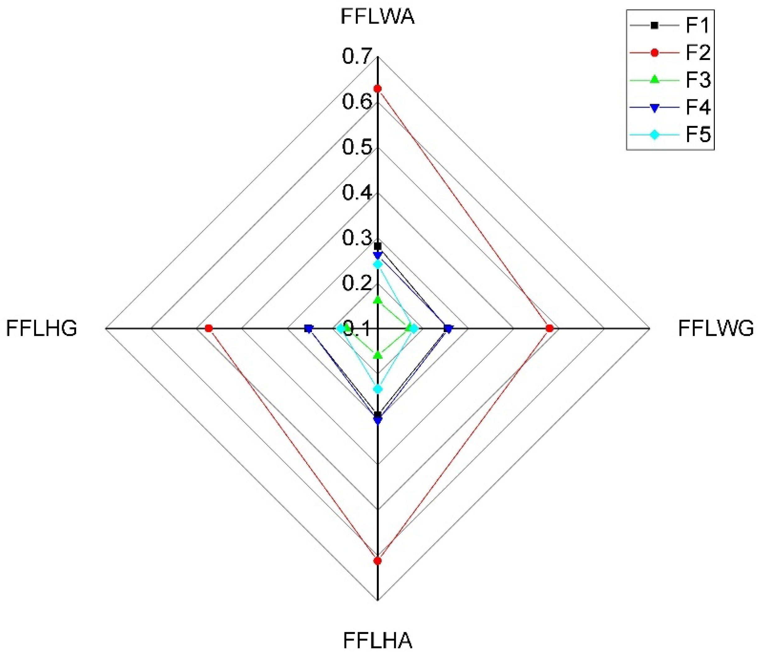
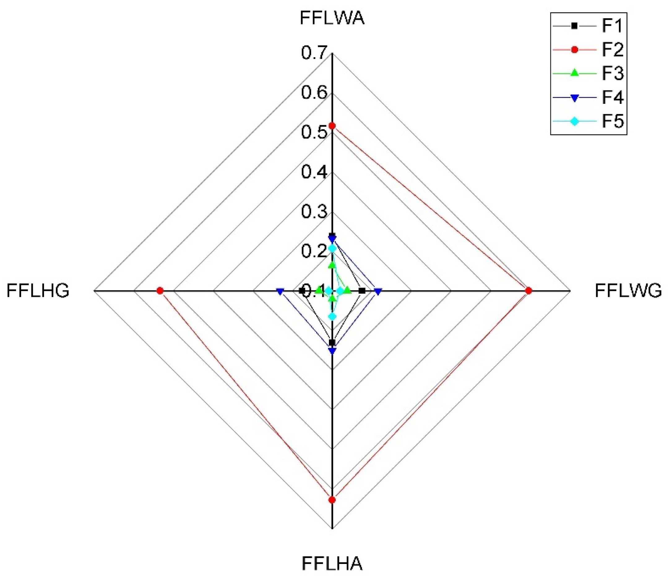
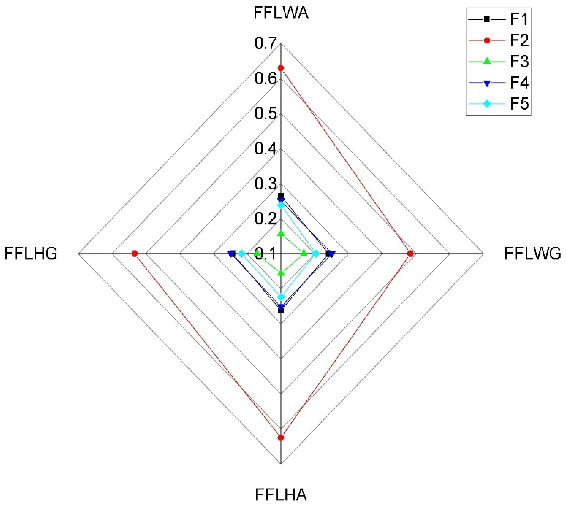
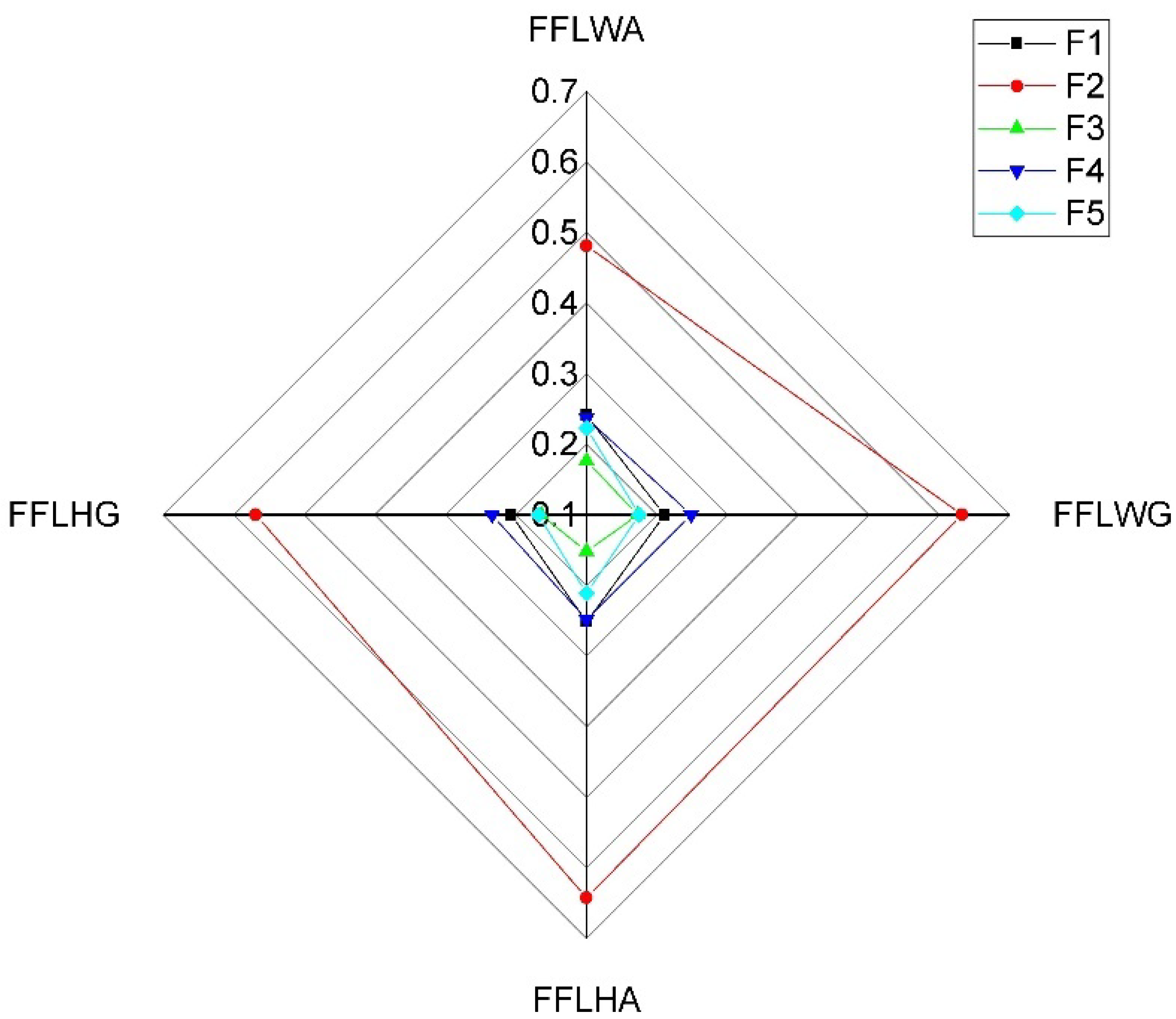
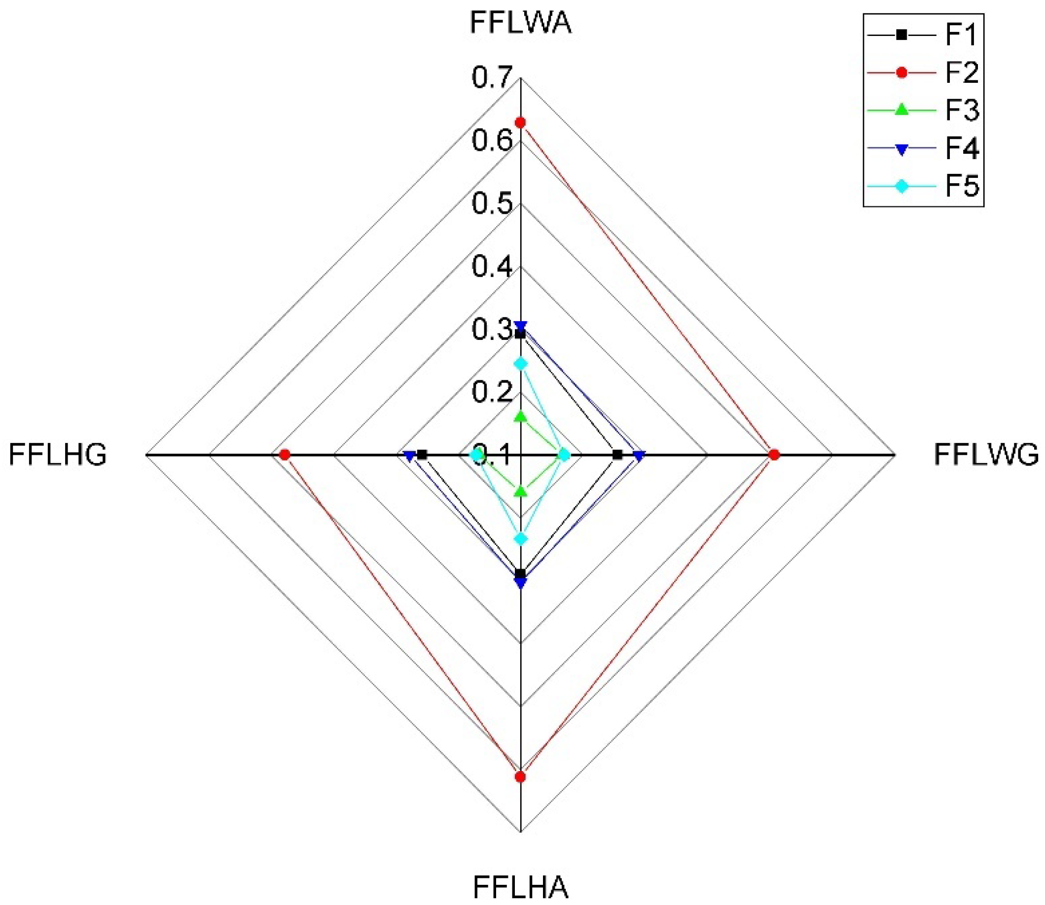
A sensitivity analysis has been conducted to better understand the impact of the various AOs on the ranking order of the alternatives with different LSFs. Figure 5, Figure 6, Figure 7, Figure 8, Figure 9 and Figure 10 have been plotted, portraying the sensitivity of the results based on various AOs taking different LSFs. As shown in Figure 5, Figure 6, Figure 7, Figure 8, Figure 9 and Figure 10, changes in the AOs and LSFs significantly influence the ranking of alternatives.

Figure 5. Sensitivity analysis for the alternatives based on FFLOWA operator in step 2 with ${\phi }^{*}={\phi }_1^{\ast }$.

Figure 6. Sensitivity analysis for the alternatives based on FFLOWG operator in step 2 with ${\phi }^{*}={\phi }_1^{\ast }$.

Figure 7. Sensitivity analysis for the alternatives based on FFLOWA operator in step 2 with ${\phi }^{*}={\phi }_2^{\ast }$.

Figure 8. Sensitivity analysis for the alternatives based on FFLOWG operator in step 2 with ${\phi }^{*}={\phi }_2^{\ast }$.

Figure 9. Sensitivity analysis for the alternatives based on FFLOWA operator in step 2 with ${\phi }^{*}={\phi }_3^{\ast }$.

Figure 10. Sensitivity analysis for the alternatives based on FFLOWG operator in step 2 with ${\phi }^{*}={\phi }_3^{\ast }$.

4.5. A Comparative Overview of the Results Based on Different AOs

In order to compare the performance of the developed AOs with existing ones, this paper uses the AOs and decision method formulated by Li et al. [53] to solve the above considered MAGDM problem. The obtained values of the closeness coefficient and ranking order of the suppliers are summarized in Table 17.

Table 17. The values of the closeness coefficient $ℭ\left({\tilde{\wp }}_i\right)$ and ranking order of the suppliers.

Aggregation Operator Used	The Closeness Coefficient Values					Ranking of the Suppliers
	$ℭ\left({\tilde{\wp }}_1\right)$	$ℭ\left({\tilde{\wp }}_2\right)$	$ℭ\left({\tilde{\wp }}_3\right)$	$ℭ\left({\tilde{\wp }}_4\right)$	$ℭ\left({\tilde{\wp }}_5\right)$
FFLWA	0.3803	0.6109	0.2222	0.3317	0.3529	$F_2\succ F_1\succ F_5\succ F_4\succ F_3$
FFLWG	0.3942	0.5856	0.2063	0.3396	0.3412	$F_2\succ F_1\succ F_5\succ F_4\succ F_3$

From Table 17, it is inferred that the best alternative obtained by the proposed approach agrees with the method formulated by Li et al. [53] which confirms the consistency of the proposed operators. It is also clear from the results summarized in Table 17 that the best alternative $\left(F_2\right)$ and the worst alternative $\left(F_3\right)$ are the same by all the approaches. However, the complete ranking order of the suppliers is slightly different from our ranking order because of the use of different aggregation operators for aggregating the preference information of the decision-makers.

In addition, Spearman’s rank correlation test [63] is used for the subsequent analyses to identify the differences between the ranking orders of the alternatives obtained by using different AOs in the formulated approach. Spearman’s rank correlation measures the strength of association of two variables. It can be defined as follows:

$$r_{SRC}=1-\frac{6{\displaystyle \sum _{j=1}^m{d}_j^2}}{m\left(m^2-1\right)},$$

where $m$ is the number of alternatives and $d$ denotes the ranking difference of alternative $F_j$ between two different rankings. According to [63], $r_{SRC}$ lies between −1 to +1. $r_{SRC}=+1$ indicates a perfect positive relationship between the two sets of rankings and $r_{SRC}=-1$ implies a perfect negative relationship between the two sets of rankings. The closer $r_{SRC}$ is to $\pm 1$, the stronger the relationship between the two rankings. Table 18, Table 19 and Table 20 summarize Spearman’s rank correlation coefficient values between different rankings obtained based on different AOs and LSFs.

Table 18. Results of Spearman’s rank correlation with ${\phi }^{*}={\phi }_1^{\ast }$.

${\phi }^{*}={\phi }_1^{\ast }$	FFLOWA+ FFLWA	FFLOWA + FFLWG	FFLOWA + FFLHA	FFLOWA + FFLHG	FFLOWG + FFLWA	FFLOWG + FFLWG	FFLOWG + FFLHA	FFLOWG + FFLHG
FFLOWA+ FFLWA	1	0.1	0.1	1	1	−0.3	0.1	−0.3
FFLOWA+ FFLWG	0.1	1	1	0.1	0.1	0.6	1	0.6
FFLOWA+ FFLHA	0.1	1	1	0.1	0.1	0.6	1	0.6
FFLOWA+ FFLHG	1	0.1	0.1	1	1	−0.3	0.1	−0.3
FFLOWG+ FFLWA	1	0.1	0.1	1	1	−0.3	0.1	−0.3
FFLOWG+ FFLWG	−0.3	0.6	0.6	−0.3	−0.3	1	0.6	1
FFLOWG+ FFLHA	0.1	1	1	0.1	0.1	0.6	1	0.6
FFLOWG+ FFLHG	−0.3	0.6	0.6	−0.3	−0.3	1	0.6	1

Table 19. Results of Spearman’s rank correlation with ${\phi }^{*}={\phi }_2^{\ast }$.

${\phi }^{*}={\phi }_1^{\ast }$	FFLOWA+ FFLWA	FFLOWA + FFLWG	FFLOWA + FFLHA	FFLOWA + FFLHG	FFLOWG + FFLWA	FFLOWG + FFLWG	FFLOWG + FFLHA	FFLOWG + FFLHG
FFLOWA+ FFLWA	1	0.1	1	0.1	1	0.1	1	0.1
FFLOWA+ FFLWG	0.1	1	0.1	1	0.1	1	0.1	1
FFLOWA+ FFLHA	1	0.1	1	0.1	1	0.1	1	0.1
FFLOWA+ FFLHG	0.1	1	0.1	1	0.1	1	0.1	1
FFLOWG+ FFLWA	1	0.1	1	0.1	0.1	0.1	1	0.1
FFLOWG+ FFLWG	0.1	1	1	1	0.1	1	0.1	1
FFLOWG+ FFLHA	1	0.1	1	0.1	1	0.1	1	0.1
FFLOWG+ FFLHG	0.1	1	0.1	1	0.1	1	0.1	1

Table 20. Results of Spearman’s rank correlation with ${\phi }^{*}={\phi }_3^{\ast }$.

${\phi }^{*}={\phi }_1^{\ast }$	FFLOWA+ FFLWA	FFLOWA+ FFLWG	FFLOWA + FFLHA	FFLOWA+ FFLHG	FFLOWG+ FFLWA	FFLOWG+ FFLWG	FFLOWG+ FFLHA	FFLOWG+ FFLHG
FFLOWA+ FFLWA	1	1	1	1	0.1	1	0.1	0.6
FFLOWA+ FFLWG	1	1	1	1	0.1	1	0.1	0.6
FFLOWA+ FFLHA	1	1	1	1	0.1	1	0.1	0.6
FFLOWA+ FFLHG	1	1	1	1	0.1	1	0.1	0.6
FFLOWG+ FFLWA	0.1	0.1	0.1	0.1	0.1	0.1	1	−0.3
FFLOWG+ FFLWG	1	1	1	1	0.1	1	0.1	0.6
FFLOWG+ FFLHA	0.1	0.1	0.1	0.1	1	0.1	1	−0.3
FFLOWG+ FFLHG	0.6	0.6	0.6	0.6	−0.3	0.6	−0.3	1

From Table 18 and Table 19, we can easily see that the ranking orders obtained using FFLOWA+ FFLWA and FFLOWG+ FFLWA have a perfect positive relationship. Similarly, Table 19 and Table 20 show that the rankings obtained by the FFLOWA+ FFLWG and FFLOWA+ FFLHG also have a perfect positive relationship.

4.6. Some Advantages and Limitations of the Proposed Approach

• The formulated approach can solve decision-making problems with qualitative information data in terms of FFLNs very efficiently.
• We can also apply this method to solve many existing decision problems with intuitionistic fuzzy linguistic and Pythagorean fuzzy linguistic information [48,49,50].
• The main limitation of this study is that it cannot handle the situations in which the attributes have some interaction and prioritization relationship between them.
• The developed study opens a new door for further research under a qualitative information environment.
• There can be some adverse situations in which the defined operational laws for FFLNs may not work. Then, we will need to undertake a further detailed investigation of the operational laws of FFLNs.

5. Conclusions

In this paper, we studied the MAGDM problems under a Fermatean fuzzy linguistic environment. To overcome the shortcomings of the existing operational laws of FFLNs, the paper has defined four new algebraic operational laws for FFLNs based on the idea of LSF. Several mathematical properties of the proposed operational laws have been studied in detail. Next, we formulated some AOs, including the FFLWA operator, the FFLWG operator, the FFLOWA operator, the FFLOWG operator, the FFLHA operator, and the FFLHG operator to aggregate different FFLNs. Furthermore, the work has proved many important properties of the proposed AOs, such as idempotency, monotonicity, commutativity, and boundedness, to establish their applicability in different areas. Utilizing the proposed AOs, the paper has developed a new decision-making approach to solve MAGDM problems with Fermatean fuzzy linguistic information. Finally, a real-life supplier selection problem has been considered to illustrate the steps of the proposed method.

In the future, we will employ the proposed AOs to solve some other decision-making problems such as medical diagnosis, pattern recognition, and image processing. Further, we will also develop some new aggregation operators such as Bonferroni mean operator, Heronian mean operator, and Hamy mean operator to aggregate the correlative Fermatean fuzzy linguistic information in future work.

References

1. Atanassov, K.T. Intuitionistic fuzzy sets. Fuzzy Sets Syst. 1986, 20, 87–96. [Google Scholar] [CrossRef]
2. Zadeh, L.A. Fuzzy sets. Inf. Control 1965, 8, 338–353. [Google Scholar] [CrossRef] [Green Version]
3. Xu, Z. Intuitionistic fuzzy aggregation operators. IEEE Trans. Fuzzy Syst. 2007, 15, 1179–1187. [Google Scholar] [CrossRef]
4. He, Y.; Chen, H.; Zhou, L.; Liu, J.; Tao, Z. Intuitionistic fuzzy geometric interaction averaging operators and their application to multi-criteria decision making. Inf. Sci. 2014, 259, 142–159. [Google Scholar] [CrossRef]
5. Ma, Z.M.; Yang, W. Symmetric intuitionistic fuzzy weighted mean operators based on weighted Archimedean t-norms and t-conorms for multi-criteria decision making. Informatica 2020, 31, 89–112. [Google Scholar] [CrossRef] [Green Version]
6. Zou, X.Y.; Chen, S.M.; Fan, K.Y. Multiple attribute decision making using improved intuitionistic fuzzy weighted geometric operators of intuitionistic fuzzy values. Inf. Sci. 2020, 535, 242–253. [Google Scholar] [CrossRef]
7. He, Y.; He, Z.; Chen, H. Intuitionistic fuzzy interaction Bonferroni means and its application to multiple attribute decision making. IEEE Trans. Cyber. 2015, 45, 116–128. [Google Scholar] [CrossRef]
8. Verma, R. Generalized Bonferroni mean operator for fuzzy number intuitionistic fuzzy sets and its application to multiattribute decision making. Int. J. Intell. Syst. 2015, 30, 499–519. [Google Scholar] [CrossRef]
9. Liu, P.; Liu, J.; Chen, M.S. Some intuitionistic fuzzy Dombi Bonferroni mean operators and their application to multi-attribute group decision making. J. Oper. Res. Soc. 2018, 69, 1–24. [Google Scholar] [CrossRef]
10. Liu, P.; Gao, H. Some intuitionistic fuzzy power Bonferroni mean operators in the framework of Dempster–Shafer theory and their application to multicriteria decision making. Appl. Soft Comput. 2019, 85, 105790. [Google Scholar] [CrossRef]
11. Verma, R.; Sharma, B.D. Intuitionistic fuzzy Einstein prioritized weighted average operators and their application to multiple attribute group decision making. Appl. Math. Inf. Sci. 2015, 9, 3095–3107. [Google Scholar] [CrossRef]
12. Ai, Z.; Xu, Z. Intuitionistic fuzzy double integrals and their fundamental properties. IEEE Trans. Fuzzy Syst. 2018, 26, 3782–3792. [Google Scholar] [CrossRef]
13. Ai, Z.; Xu, Z. Line integrals of intuitionistic fuzzy calculus and their properties. IEEE Trans. Fuzzy Syst. 2018, 26, 1435–1446. [Google Scholar] [CrossRef]
14. Ai, Z.; Xu, Z. Multiple definite integrals of intuitionistic fuzzy calculus and isomorphic mappings. IEEE Trans. Fuzzy Syst. 2018, 26, 670–680. [Google Scholar] [CrossRef]
15. Zhang, H.; Yu, L. New distance measures between intuitionistic fuzzy sets and interval-valued fuzzy sets. Inf. Sci. 2013, 245, 181–196. [Google Scholar] [CrossRef]
16. Ngan, R.T.; Son, L.H.; Cuong, B.C.; Ali, M. H-max distance measure of intuitionistic fuzzy sets in decision making. Appl. Soft Comput. J. 2018, 69, 393–425. [Google Scholar] [CrossRef]
17. Mahanta, J.; Panda, S. A novel distance measure for intuitionistic fuzzy sets with diverse applications. Int. J. Intell. Syst. 2021, 36, 615–627. [Google Scholar] [CrossRef]
18. Hao, Z.; Xu, Z.; Zhao, H.; Zhang, R. The context-based distance measure for intuitionistic fuzzy set with application in marine energy transportation route decision making. Appl. Soft Comput. 2021, 101, 107044. [Google Scholar] [CrossRef]
19. Song, Y.; Wang, X.; Quan, W.; Huang, W. A new approach to construct similarity measure for intuitionistic fuzzy sets. Soft Comput. 2019, 23, 1985–1998. [Google Scholar] [CrossRef]
20. Boran, F.E.; Akay, D. A biparametric similarity measure on intuitionistic fuzzy sets with applications to pattern recognition. Inf. Sci. 2014, 255, 45–57. [Google Scholar] [CrossRef]
21. Raji-Lawal, H.Y.; Akinwale, A.T.; Folorunsho, O.; Mustapha, A.O. Decision support system for dementia patients using intuitionistic fuzzy similarity measure. Soft Comput. Lett. 2020, 2, 100005. [Google Scholar] [CrossRef]
22. Singh, A.; Kumar, S. A novel dice similarity measure for IFSs and its applications in pattern and face recognition. Expert Syst. Appl. 2020, 149, 113245. [Google Scholar] [CrossRef]
23. Verma, R.; Sharma, B.D. Exponential entropy on intuitionistic fuzzy sets. Kybernetika 2013, 49, 114–127. [Google Scholar]
24. Verma, R.; Sharma, B.D. On intuitionistic fuzzy entropy of order-α. Adv. Fuzzy Syst. 2014, 1–8. [Google Scholar] [CrossRef] [Green Version]
25. Verma, R.; Sharma, B.D. R-norm entropy on intuitionistic fuzzy sets. J. Intell. Fuzzy Syst. 2015, 28, 327–335. [Google Scholar] [CrossRef]
26. Thao, N.X. Some new entropies and divergence measures of intuitionistic fuzzy sets based on Archimedean t-conorm and application in supplier selection. Soft Comput. 2021, 25, 5791–5805. [Google Scholar] [CrossRef]
27. Verma, R.; Sharma, B.D. On generalized intuitionistic fuzzy divergence (relative information) and their properties. J. Uncertain Syst. 2012, 6, 308–320. [Google Scholar]
28. Verma, R.; Sharma, B.D. Intuitionistic fuzzy Jensen-Rényi divergence: Applications to multiple-attribute decision making. Informatica 2013, 37, 399–409. [Google Scholar]
29. Mishra, A.R.; Singh, R.K.; Motwani, D. Intuitionistic fuzzy divergence measure-based ELECTRE method for performance of cellular mobile telephone service providers. Neural Comput. Appl. 2020, 32, 3901–3921. [Google Scholar] [CrossRef]
30. Verma, R.; Sharma, B.D. A new measure of inaccuracy with its application to multi-criteria decision making under intuitionistic fuzzy environment. J. Intell. Fuzzy Syst. 2014, 27, 1811–1824. [Google Scholar] [CrossRef]
31. Yager, R.R. Pythagorean fuzzy subsets. In Proceedings of the Joint IFSA World Congress and NAFIPS Annual Meeting, Edmonton, AB, Canada, 24–28 June 2013; pp. 57–61. [Google Scholar]
32. Yager, R.R.; Abbasov, A.M. Pythagorean membership grades, complex numbers, and decision making. Int. J. Intell. Syst. 2013, 28, 436–452. [Google Scholar] [CrossRef]
33. Zhang, X.; Xu, Z. Extension of TOPSIS to multiple criteria decision making with Pythagorean fuzzy sets. Int. J. Intell. Syst. 2014, 29, 1061–1078. [Google Scholar] [CrossRef]
34. Yager, R.R. Pythagorean membership grades in multicriteria decision making. IEEE Trans. Fuzzy Syst. 2014, 22, 958–965. [Google Scholar] [CrossRef]
35. Wei, G.; Lu, M. Pythagorean fuzzy power aggregation operators in multiple attribute decision making. Int. J. Intell. Syst. 2018, 33, 169–186. [Google Scholar] [CrossRef]
36. Yang, Y.; Chin, K.; Ding, H.; Lv, H.; Li, Y. Pythagorean fuzzy Bonferroni means based on T-norm and its dual T-conorm. Int. J. Intell. Syst. 2019, 34, 1303–1336. [Google Scholar] [CrossRef]
37. Akram, M.; Ilyas, F.; Al-Kenani, N.A. Two-phase group decision-aiding system using ELECTRE III method in Pythagorean fuzzy environment. Arab. J. Sci. Eng. 2021, 46, 3549–3566. [Google Scholar] [CrossRef]
38. Ejegwa, P.A. Modified Zhang and Xu’s distance measure for Pythagorean fuzzy sets and its application to pattern recognition problems. Neural Comput. Appl. 2020, 32, 10199–10208. [Google Scholar] [CrossRef]
39. Molla, M.U.; Giri, B.C.; Biswas, P. Extended PROMETHEE method with Pythagorean fuzzy sets for medical diagnosis problems. Soft Comput. 2021, 25, 4503–4512. [Google Scholar] [CrossRef]
40. Bakioglu, G.; Atahan, A.O. AHP integrated TOPSIS and VIKOR methods with Pythagorean fuzzy sets to prioritize risks in self-driving vehicles. Appl. Soft Comput. 2021, 99, 106948. [Google Scholar] [CrossRef]
41. Senapati, T.; Yager, R.R. Fermatean fuzzy sets. J. Ambient Intell. Humaniz. Comput. 2019. [Google Scholar] [CrossRef]
42. Senapati, T.; Yager, R.R. Some new operations over Fermatean fuzzy numbers and application of Fermatean fuzzy WPM in multiple criteria decision making. Informatica 2019, 30, 391–412. [Google Scholar] [CrossRef] [Green Version]
43. Senapati, T.; Yager, R.R. Fermatean fuzzy weighted averaging/geometric operators and its application in multi-criteria decision-making methods. Eng. Appl. Artif. Intell. 2019, 85, 112–121. [Google Scholar] [CrossRef]
44. Aydemir, S.B.; Yilmaz Gunduz, S. Fuzzy TOPSIS method with Dombi aggregation operators and its application in multi-criteria decision making. J. Intell. Fuzzy Syst. 2020, 39, 851–869. [Google Scholar] [CrossRef]
45. Mishra, A.R.; Rani, P.; Pandey, K. Fermatean fuzzy CRITIC-EDAS approach for the selection of sustainable third-party reverse logistics providers using improved generalized score function. J. Ambient. Intell. Humaniz. Comput. 2021, 1, 1. [Google Scholar] [CrossRef]
46. Zadeh, L.A. The concept of a linguistic variable and its application to approximate reasoning—II. Inf. Sci. 1975, 8, 301–357. [Google Scholar] [CrossRef]
47. Zadeh, L.A. The concept of a linguistic variable and its application to approximate reasoning-III. Inf. Sci. 1975, 9, 43–80. [Google Scholar] [CrossRef]
48. Wang, J.B.; Li, H.B. Multi-criteria decision-making method based on aggregation operators for intuitionistic linguistic fuzzy numbers. Control Decis. 2010, 25, 1571–1574. [Google Scholar]
49. Liu, P. Some generalized dependent aggregation operators with intuitionistic linguistic numbers and their application to group decision making. J. Comput. Syst. Sci. 2013, 79, 131–143. [Google Scholar] [CrossRef] [Green Version]
50. Liu, P.; Wang, Y. Multiple attribute group decision making methods based on intuitionistic linguistic power generalized aggregation operators. Appl. Soft Comput. J. 2014, 17, 90–104. [Google Scholar] [CrossRef]
51. Su, W.; Li, W.; Zeng, S.; Zhang, C. Atanassov’s intuitionistic linguistic ordered weighted averaging distance operator and its application to decision making. J. Intell. Fuzzy Syst. 2014, 26, 1491–1502. [Google Scholar] [CrossRef]
52. Yu, S.; Wang, J.; Wang, J. An extended TODIM approach with intuitionistic linguistic numbers. Int. Trans. Oper. Res. 2018, 25, 781–805. [Google Scholar] [CrossRef]
53. Liu, D.; Liu, Y.; Chen, X. Fermatean fuzzy linguistic set and its application in multicriteria decision making. Int. J. Intell. Syst. 2019, 34, 878–894. [Google Scholar] [CrossRef]
54. Liu, D.; Liu, Y.; Wang, L. Distance measure for Fermatean fuzzy linguistic term sets based on linguistic scale function: An illustration of the TODIM and TOPSIS methods. Int. J. Intell. Syst. 2019, 34, 2807–2834. [Google Scholar] [CrossRef]
55. Herrera, F.; Martínez, L. A model based on linguistic 2-tuples for dealing with multigranular hierarchical linguistic contexts in multi-expert decision-making. IEEE Trans. Syst. Man Cybern. Part B Cybern. 2001, 31, 227–234. [Google Scholar] [CrossRef] [Green Version]
56. Xu, Z. Intuitionistic preference relations and their application in group decision making. Inf. Sci. 2007, 177, 2363–2379. [Google Scholar] [CrossRef]
57. Wang, J.Q.; Wu, J.T.; Wang, J.; Zhang, H.Y.; Chen, X.H. Interval-valued hesitant fuzzy linguistic sets and their applications in multi-criteria decision-making problems. Inf. Sci. 2014, 288, 55–72. [Google Scholar] [CrossRef]
58. Liao, H.; Qin, R.; Gao, C.; Wu, X.; Hafezalkotob, A.; Herrera, F. Score-HeDLiSF: A score function of hesitant fuzzy linguistic term set based on hesitant degrees and linguistic scale functions: An application to unbalanced hesitant fuzzy linguistic MULTIMOORA. Inf. Fusion 2019, 48, 39–54. [Google Scholar] [CrossRef]
59. Yager, R.R. On ordered weighted averaging aggregation operators in multicriteria decision making. IEEE Trans. Syst. Man Cybern. 1988, 18, 183–190. [Google Scholar] [CrossRef]
60. Chiclana, F.; Herrera, F.; Herrera-Viedma, E. The ordered weighted geometric operator: Properties and application in MCDM problems. In Proceedings of the 8th Conference Information Processing and Management of Uncertainty in Knowledge based Systems (IPMU), Madrid, Spain, 3–7 July 2000; pp. 985–991. [Google Scholar]
61. Xu, Z.; Da, Q.L. An overview of operators for aggregating information. Int. J. Intell. Syst. 2003, 18, 953–969. [Google Scholar] [CrossRef]
62. Xu, Z. An overview of methods for determining OWA weights. Int. J. Intell. Syst. 2005, 20, 843–865. [Google Scholar] [CrossRef]
63. Parkan, C.; Wu, M.L. Decision-making and performance measurement models with applications to robot selection. Comput. Ind. Eng. 1999, 36, 503–523. [Google Scholar] [CrossRef]