Predicting Missing Seismic Velocity Values Using Self-Organizing Maps to Aid the Interpretation of Seismic Reflection Data from the Kevitsa Ni-Cu-PGE Deposit in Northern Finland

Abstract

We use self-organizing map (SOM) analysis to predict missing seismic velocity values from other available borehole data. The site of this study is the Kevitsa Ni-Cu-PGE deposit within the mafic-ultramafic Kevitsa intrusion in northern Finland. The site has been the target of extensive seismic reflection surveys, which have revealed a series of reflections beneath the Kevitsa resource area. The interpretation of these reflections has been complicated by disparate borehole data, particularly because of the scarce amount of available sonic borehole logs and the varying practices in logging of borehole lithologies. SOM is an unsupervised data mining method based on vector quantization. In this study, SOM is used to predict missing seismic velocities from other geophysical, geochemical, geological, and geotechnical data. For test boreholes, for which measured seismic velocity logs are also available, the correlation between actual measured and predicted velocities is strong to moderate, depending on the parameters included in the SOM analysis. Predicted reflectivity logs, based on measured densities and predicted velocities, show that some contacts between olivine pyroxenite/olivine websterite-dominant host rocks of the Kevitsa disseminated sulfide mineralization—and metaperidotite—earlier extensively used “lithology” label that essentially describes various degrees of alteration of different olivine pyroxenite variants—are reflective, and thus, alteration can potentially cause reflectivity within the Kevitsa intrusion.

1. Introduction

Typically, mining and exploration environments are targets of intensive drilling for resource estimation and feasibility studies, and commonly, in addition to lithology, drill hole logging includes geochemical assays and geotechnical analyses and parameters. Specific gravity (SG) measurements of the drill core are quite common, as well as downhole logging of magnetic susceptibility, natural gamma, electrical resistivity, self potential (SP), and induced polarization (IP). Gamma-gamma density logs are less common as they require handling of a radioactive source, and sonic logs are even rarer due to their less recognized benefits. In general, borehole datasets from mining and exploration environments are typically much localized and incomplete from the point of view of interpreting the causes of geophysical anomalies, in particular anomalous seismic properties, and they limit the success of geophysical mineral exploration efforts.

Recently, data mining approaches, such as the self-organizing map (SOM; [1,2]) analysis employed in this study, have been increasingly used for analyses of the disparate and multivariate geoscientific datasets that are typical for mining and exploration environments (e.g., [3,4,5,6,7,8,9,10]). SOM is an artificial neural network that works on a vector quantization methodology allowing unsupervised analysis, i.e., no prior information is needed on the type or number of groupings within the data, to determine the underlying linear and non-linear relationships amongst different data. Typically 2D “maps” are used to visualize the underlying statistical relationships between the variables, which makes interpretation of the complex multidimensional data more effective (e.g., [11]). Major strengths of the methodology include the robust handling of sparse and disparate input data, labels, incomplete data, and the ability to predict missing data values for such data (e.g., [12,13,14]).

Extensive seismic reflection data have been collected at the Kevitsa Ni-Cu-PGE deposit that is located in northern Finland (Figure 1). These data include four intersecting 2D seismic reflection profiles acquired in 2007 as a part of High-Resolution Reflection Seismics for Ore Exploration (HIRE) 2007–2010 project that aimed at testing the applicability of seismic exploration method in Kevitsa [16,17] and a 3D seismic reflection survey conducted in 2010 for mine planning and deep mineral exploration purposes [18,19]. Laterally continuous reflections were observed in the seismic data from 200–300 m depth to about 1 km depth within a constrained region inside the intrusion (Figure 2), beneath the resource area. These reflections were originally interpreted to originate from contacts between the tops and bottoms of internally differentiated magmatic layers (Figure 3; [17,18,19,20]) that had been suggested to control the extent of economic mineralization in Kevitsa just before the 3D reflection seismic survey took place in 2010 [21,22]. However, this interpretation was not fully supported by the borehole data (e.g., [10,20]). In particular, only very little plagioclase-bearing olivine websterite, constituting the tops of the suggested magmatic layers, was logged from the borehole data to trace such layering that would result in the observed continuous reflections. At the time, this was partly attributed to varying geological logging practices, especially the earlier usage of “metaperidotite” as a lithological label to describe amphibole-altered (in various degrees) olivine pyroxenite variants (pyroxenite, olivine pyroxenite, websterite, olivine websterite, and plagioclase-bearing olivine websterite) that constitute the suggested magmatic layers (e.g., [20]). This essentially means that the lithological logs and the alteration logs are not consistent and lack crucial information from the point of view of seismic interpretation. Another complicating factor for the seismic interpretation in the area has been that sonic borehole logs are available from 16 sparsely placed boreholes, and only about half of these boreholes are located in the area of the observed reflectivity (i.e., resource area in Figure 1).

In this study, we use SOM to predict missing seismic velocity data values in the Kevitsa borehole data in order to aid the interpretation of the potential causes of the observed reflectivity within the Kevitsa intrusion. We use SOM to predict missing seismic velocity values, which are crucial to seismic interpretation, using available geophysical, geochemical, geological, and geotechnical logging data in different combinations. For test boreholes, for which measured seismic velocity logs are also available, the correlation between actual measured and predicted seismic velocity values is mostly strong to moderate. Based on the reflectivity logs, derived from measured densities and predicted velocities for boreholes that do not contain actual seismic velocity measurements, some alternating layers of olivine pyroxenite/olivine websterite and metaperidotite seem reflective. Thus, based on the results, it appears that alteration can potentially cause reflectivity within the Kevitsa intrusion.

This work focuses on the SOM velocity predictions, and the results of this study are further utilized in a study by Junno et al. [10] that presents extensive SOM borehole data analyses on the role of lithological variation and alteration on the reflectivity properties, as well as theoretical modeling of the effect of alteration and mineral composition on the reflectivity properties of the Kevitsa rock types. In line with the results of this work, Junno et al. [10] conclude that the observed reflectivity within the Kevitsa intrusion can be attributed to alteration, possibly associated with the sulfide mineralization, rather than to the earlier suggested magmatic layering.

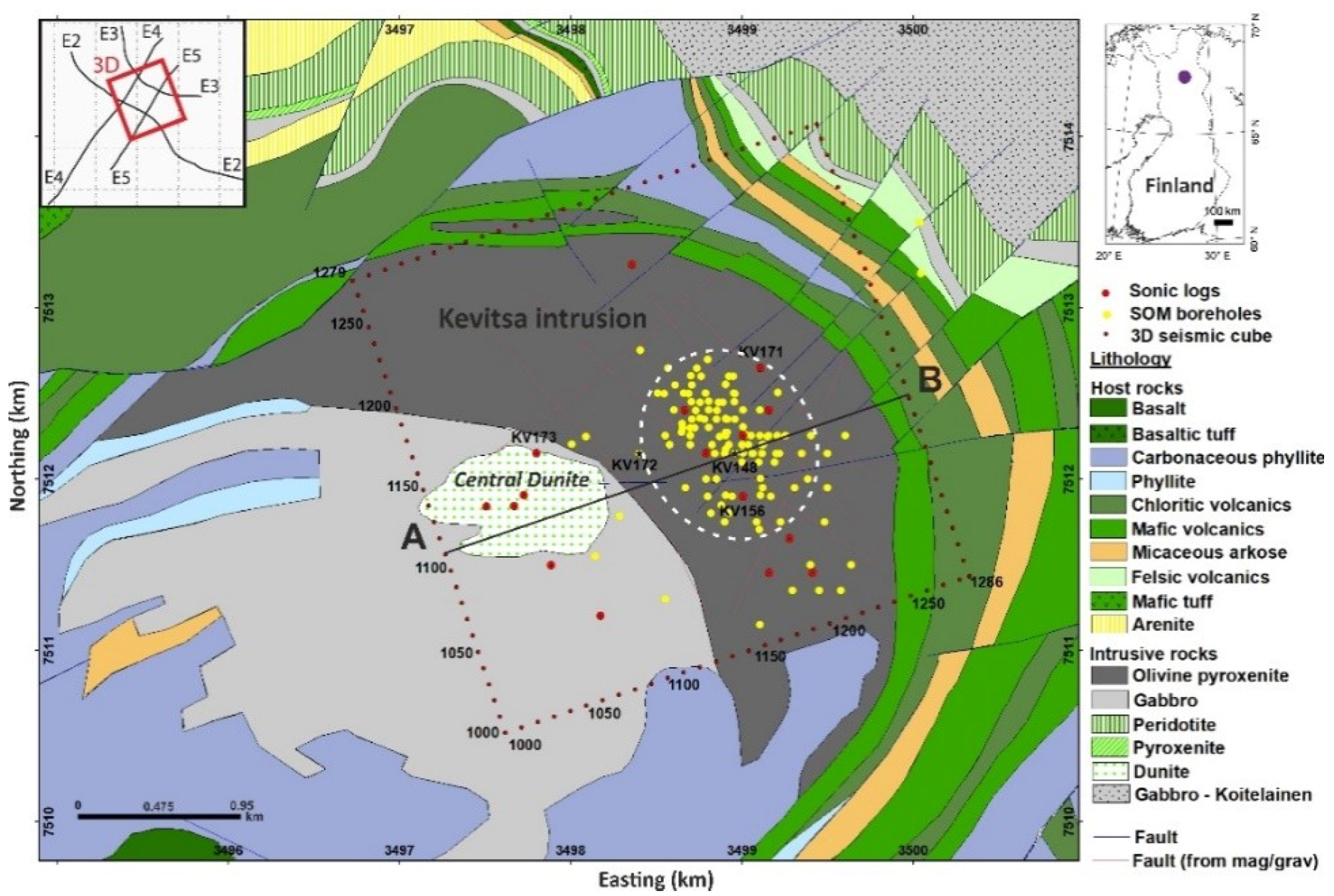
2. Geological Background

The mafic-ultramafic Kevitsa intrusion is located within the Central Lapland Greenstone Belt (CLGB) in northern Finland (Figure 1) and hosts a large disseminated Ni-Cu-PGE sulfide deposit [23,24]. The CLGB rocks are of Paleoproterozoic age and consist of metamorphosed and hydrothermally altered volcano-sedimentary rocks. The Kevitsa intrusion is dated at about 2.06 Ga [23,24] and consists of gabbroic rocks in the southwest and olivine pyroxenite and its variants in the northeast, with several dunite units sitting within and around the intrusion (e.g., central dunite in Figure 1). At the surface, the intrusion covers an area of about 16 km² [23], and it reaches about 1.5 km depth at its deepest parts [17,20]. The Kevitsa open-pit mine commenced in 2012 and is currently operated by Boliden AB. For more detailed geological description of the Kevitsa complex, the reader is referred to [23,24,25].

At around the time of the Kevitsa 3D reflection seismic survey it was suggested [21,22] that the extent of economic mineralization in Kevitsa is controlled by the extent of smaller-scale magmatic layers that are internally differentiated (Figure 3) and laterally restricted to the resource area. This magmatic layering hypothesis gained support from the seismic reflection studies [17,18,19,20], which showed laterally continuous reflections in the Kevitsa 2D and in particular in the 3D seismic reflection data within a limited region inside the intrusion (Figure 2). These reflections were interpreted to originate from the sharp contacts between tops and bottoms of the magmatic layers (Figure 3). On average, the contrast between the physical properties of plagioclase-bearing olivine websterite, the tops of the suggested magmatic layers, and olivine pyroxenite, the bottoms, is enough to produce detectable reflections (Figure 4). However, this interpretation was not unequivocally supported by the borehole data, with only a handful of samples (1.3% of the selected samples used in this study) logged as plagioclase-bearing olivine websterite [10,20,22]. In particular, these samples were not observed to form consistent, traceable layers from one borehole to another. Identification of the individual layers is complicated by the presence of the widespread amphibole alteration of olivine pyroxenite and its variants that were earlier logged as “metaperidotite” [23] in the lithology field rather than in the “alteration” field. The metaperidotite masks the identification of the primary lithology, and thus, the problems of identifying traceable magmatic layers were initially attributed to inconsistent logging practices. However, as recent geological works by [26,27] do not anymore support the idea of continuous smaller-scale magmatic layering within the resource area, it now seems that the evidence for obvious layering is lacking altogether. Individual horizons are inconsistent between boreholes based on lithology, whole-rock compositions, and ore grades [27]. This reopens the question about origin of the observed reflectivity within the Kevitsa intrusion (Figure 2) for scrutiny.

3. Materials and Methods

3.1. Kevitsa Borehole Data

Extensive geoscientific investigations have been conducted in Kevitsa since the discovery in 1987. The available data include 2D and 3D seismic reflection data [17,18] and extensive borehole data that are utilized in this study. In total, more than 900 boreholes have been drilled within and around the Kevitsa resource area. These borehole data include comprehensive loggings for selected geochemical assays and lithology. However, only about 134 boreholes contain geophysical data (see below for details). Furthermore, sonic borehole logs are available from 16 boreholes, out of which only nine are located within the resource area. The missing data pose a problem, since the borehole data offer only localized and incomplete description of the subsurface for a comprehensive seismic interpretation.

For the current study, representative boreholes were selected from the available vast borehole dataset. Priority was given to boreholes that contain geophysical data. Selected samples had to have measurements for at least one geophysical parameter. In addition, selected boreholes had to be at least 300 m deep. This is because the overall aim of this study is to aid the interpretation of the 3D seismic reflection data where the observed reflectivity is poor up to 200–300 m depth due to the high background velocity of the Kevitsa intrusion (greater than 6500 m/s) and issues with the sampling of the seismic wavefield at shallow depths (and low seismic fold). Most of the boreholes are located within the Kevitsa resource area, but exceptions were made for boreholes containing geophysical data, especially sonic borehole logs. In total, 134 boreholes were selected, out of which 108 boreholes are located within the resource area (Figure 1). Finally, a simple nearest-neighbor interpolation method was used to re-sample the borehole data to uniform one-meter (1 m) downhole intervals in order to compile the data into one file for the SOM analyses. This resulted in 64,999 samples.

Selected Parameters for the Analyses

In total, nine geophysical and geotechnical parameters were selected for the analyses from the borehole data (

Table 1. Different parameters used in SOM. In total 134 boreholes were selected for the SOM analysis. Listed in the table are the parameter (unit in brackets) and the number indicating from how many boreholes these parameters were available. In addition, the missing percentage was calculated for each parameter. The missing percentage is the percentage of samples with missing measurements for the given parameter out of the total amount of samples (64,999).

Parameter	Number of Boreholes	Missing Percentage (%)
Geophysical and geotechnical
Vp (m/s)	16	81.5
Vs (m/s)	14	84.8
Density (kg/m3)	16	81.8
SG (kg/m3)	105	28.3
RQD (pct)	13	87.5
Natural gamma (µR/h)	64	47.7
Magnetic susceptibility (10−3 SI)	13	87.9
Electrical resistivity (Ohmm)	60	51.3
IP (pct)	59	52.3
Geochemical
Ni (pct)	132	10.9
Cu (pct)	132	10.9
Au (ppb)	132	32.4
Pd (ppb)	131	34.1
Pt (ppb)	124	47.0
Fe (pct)	132	10.9
S (pct)	132	10.9
Co (ppm)	132	10.9
Cr (ppm)	132	10.9
Al (pct)	45	73.6
Mg (pct)	45	73.6
Ca (pct)	45	73.6
Na (pct)	45	73.6
Labels
Lithological	134	0.7
Alteration	60	58.5

). These were P- and S-wave velocities (Vp and Vs, respectively), gamma-gamma density, specific gravity (SG), rock-quality designation (RQD), natural gamma, electrical resistivity, induced polarization (IP) effect and magnetic susceptibility. Many factors influence the reflectivity, but the governing parameter is the acoustic impedance difference between lithologies. Acoustic impedance (Z) is the product of seismic velocity (V) and density ($\rho )$

$$Z=V\ast \rho$$

(1)

The reflection coefficient (R), i.e., the ratio of reflected to incident energy, is in the simplest case of vertical incidence between upper (u) and lower (l) medium

$$R=\frac{Z_l-Z_u}{Z_l+Z_u}$$

(2)

Generally, a reflection coefficient of 6% is thought to be enough for a detectable reflection [28,29].

Geochemical parameters selected were nickel (Ni), copper (Cu), iron (Fe), sulfur (S), cobalt (Co), chromium (Cr), gold (Au), platinum (Pt), and palladium (Pd). These form the main sulfide minerals present in Kevitsa (pyrrhotite, pentlandite, chalcopyrite, and several platinum group minerals). In addition, aluminum (Al), magnesium (Mg), calcium (Ca) and sodium (Na) were added as indicators of magmatic layering—with high-Al related to plagioclase-bearing olivine websterite and high-Mg to olivine pyroxenite—and alteration—high-Ca and -Na concentrations are proxies for alteration.

Only a few samples (1221) selected for the analyses contain all the selected geophysical parameters, and most of the samples (31,300) contain only one geophysical measurement (usually SG; Table 1). Selected geochemical assays (Table 1) have been measured quite comprehensively, whereas most of the geophysical parameters are missing in over 80% of the samples. An exception to this is SG, which is only missing in 28.3% of samples selected for the analyses. In addition, natural gamma, electrical resistivity, and IP have been measured for almost half of the samples (Table 1). Magnetic susceptibility is missing for 87.9% of the selected samples.

Lithological labels and alteration were also included into the analyses. Lithology has been logged for almost all of the selected samples (with only 0.7% of the samples missing lithological labels; Table 1), whereas alteration has been logged for less than half of the samples (for 41.5% of the samples chosen for the analyses; Table 1). However, it should be noted again that the lithological labels also include the metaperidotite label that describes alteration, not primary lithology. It should also be noted that if alteration is not logged for a given sample, it does not mean that the sample is not altered, but simply indicates missing information on the alteration assemblages. These inconsistencies in the logging of lithologies and alteration complicate the interpretation of the reflectivity properties in terms of the lithology and alteration. Originally, there were more than 70 different lithological labels used for the borehole data, and these were re-organized and simplified into 18 different classes. Host rocks (in total only about 2.5% of all lithology labels for the selected samples were labelled as host rocks) contained 56 different labels and these were subdivided into just two host rock groups, metavolcanics and metasediments, which both have very similar petrophysical properties (Figure 4). About 90% of all lithology labels were of different olivine pyroxenite variants (pyroxenite, olivine pyroxenite, websterite, olivine websterite, and plagioclase-bearing olivine) and metaperidotite. The lithological labels for these rock types were respected (i.e., left as they were originally logged). About 4% of the lithology labels were dunite labels. These were subdivided into three groups; (1) central dunite, consisting of dunite and peridotite situated within the central dunite unit (Figure 1), (2) footwall dunite consisting of dunite at the basal contact of the intrusion, and (3) dunite consisting of dunite situated within the main intrusion (e.g., [21,22]). Other rock groups (2.8% of all labels) include dykes, veins, xenoliths, sulfide veins, and fracture zones, and they were left as they were originally logged. Samples with missing lithology information (0.7% of the selected samples) were left empty (no label). Alteration consisted of 12 different labels out of which amphibole and serpentinite were the most common labels (about 82% amphibole and 4% serpentinite).

The categorical parameters, i.e., the lithological labels and alteration, were converted into binary parameters (all samples were given a value 1 or 0 depending if the sample was of the given lithology or alteration unit or not) for the SOM analyses. This resulted in 19 lithological parameters (18 actual lithological labels + “no lithology” label) and 13 alteration parameters (12 actual alteration labels + “no alteration logged” label).

3.2. Self-Organizing Map Analysis

A self-organizing map (SOM; [1,2]) is a type of an artificial neural network (ANN) that is trained using unsupervised learning to produce a discrete low dimensional representation, typically 2D plot or ”map”, of complex high-dimensional input data. SOM combines vector projection and vector quantization methods. It applies competitive learning as opposite to other ANNs that use error-correction learning, and it uses a neighborhood function in order to preserve the topological properties of the input data space. Major strengths of the methodology include robust handling of multivariate, disparate, and incomplete input data, as well as categorical parameters, such as lithological labels (e.g., [12,13,14]). SOM is used for several functions, such as prediction, clustering, pattern recognition, and classification, operating on large volumes of data. SOM analysis has been widely used for different applications in different research fields [30,31,32], and recently it has been also applied to hard rock mineral exploration (e.g., [3,4,5,6,7,8,9,10]). Commonwealth Scientific and Industrial Research Organization (CSIRO)’s self-organizing map software (SiroSOM; [33]), which is based on a Matlab SOM Toolbox [34,35], is employed in this study. For the comprehensive information on the principles of the SOM, the reader is referred to [1,2,35].

A SOM consists of nodes organized on a typically 2D regular-spaced hexagonal or rectangular grid. The number of nodes is user-specific and determined at the initialization of SOM. An n-dimensional (nD) node vector (n_x = [n₁, ..., n_n]) is associated with each node. The dimensionality (n) of the node vector is equal to the dimension of the input data vectors (in SOM, the input data samples are treated as nD data vectors (d)), which is the number of parameters associated with the input data. A neighborhood function connects each node vector to its neighboring node vectors and dictates the structure of the SOM. The SOM shape is often a sheet shape, but cylinder and toroid shapes can also be used. An iterative two-step learning process is used to train the node vectors to represent the original spatial distribution of the input data vectors in the nD data space. In the first, competitive learning step, the similarity between a randomly selected starting input data vector and all the node vectors of SOM is typically measured using, Euclidean distance. The node which vector is the most similar, i.e., the closest, to the starting input data vector is the “winner node” and is called the best-matching unit (BMU; denoted here by w),

$$\Vert d-n_w\Vert =\underset{i}{\min }\left\{\Vert d-n_i\Vert \right\}$$

(3)

The BMU moves even closer to the selected input data vector in the nD data space. In the next, co-operative learning step, the neighbors of the BMU also move closer to the selected input data vector, but with lesser amount depending on the learning rate $\alpha \left(t\right)$ and distance from the BMU. The amount of movement related to the node vector of unit i is

$$n_i\left(t+1\right)=n_i\left(t\right)+\alpha \left(t\right)h_{wi}\left(t\right)\left[d\left(t\right)-n_i\left(t\right)\right]$$

(4)

where t is time, $d\left(t\right)$ is a random data vector at time t, and $h_{wi}\left(t\right)$ is the neighborhood function around the winner node w at time t [34]. The neighborhood function tells how strongly the nodes are connected to each other, and the most common neighborhood function is “Gaussian” neighborhood function [35]

$$h_{wi}\left(t\right)=e^{\left(\frac{-d_{wi}^2}{2{\sigma }_t^2}\right)}$$

(5)

where ${\sigma }_t$ is the neighborhood radius, and $d_{wi}=\Vert r_w-r_i\Vert$ is the distance between units w and i. The learning process is repeated several times for each input data vector with reducing learning rate and neighborhood radius. After training, the node vectors are situated within the original input data vectors in the nD data space, and each node vector represents a group (since usually there are more data vectors than node vectors) of the data vectors closest to it. Several node vectors close together can form subsets of a larger group or cluster. Regression is used to project the node vectors from nD space onto a 2D space. This process preserves the topology of the node vectors. The underlying statistical relations between different data can be imaged on a 2D plot (or “map”) that helps the interpretation of the multidimensional data (e.g., [4,11,33]).

SOM can be used to predict missing values for the incomplete datasets (e.g., [12,13,14]). In SOM, the BMUs for each data vector with missing data values are calculated based on the available data. After the SOM training, missing values can be calculated and filled in according to the BMU and the distance of the data vector from the node vector corresponding to the BMU. In this study, after extensive testing, a SOM size of 48 × 40 was selected, which yielded to 1920 node vectors. These node vectors were randomly distributed at the beginning of SOM analyses and trained to represent the original distribution of the input data. These vectors were clustered, and the missing data values were imputed trough five more iterations.

4. Results

Predicting Missing Seismic Velocities Using SOM

Several SOM tests were run using different parameters in different combinations (selection of these runs are shown in

Table 2. Different sets of parameters used for different SOM runs (1–18) to predict missing seismic velocity values for boreholes KV171, KV173, and KV156. Correlation coefficients between actual measured and predicted SOM logs are shown for both Vp (CC_Vp) and Vs (CC_Vs). The runs that resulted in correlations greater than 0.70 are highlighted in yellow, those with correlation greater than 0.60 but smaller than 0.70 are highlighted in green, and those with correlations greater than 0.50 but smaller than 0.60 in blue. Predicted velocities from run 9 are shown in Figure 5, Figure 6 and Figure 7. Den = density; NG = natural gamma; Susc = magnetic susceptibility; Res = electrical resistivity; GChem1 = geochemical parameters Ni, Cu, Au, Pd, Pt, Fe, S, Co, Cr, Al, Ca, Mg, and Na; GChem2 = geochemical parameters Ni, Cu, Au, Pd, Pt, Fe, S, C, and Cr; Lith1 = lithology; Lith2 = lithology without metaperidotite label; Alt = alteration; x = parameter included in the run.

Run	Vp	Vs	NG	Den	SG	RQD	Susc	Res	IP	GChem1	GChem2	Lith1	Lith2	Alt	KV171		KV173		KV156
															CCVp	CCVs	CCVp	CCVs	CCVp	CCVs
1	x	x	x	x	x	x	x	x	x	x		x		x	0.65	0.66	0.74	0.81	0.56	0.64
2	x	x	x	x	x	x	x	x	x	x		x			0.57	0.64	0.79	0.87	0.58	0.60
3	x	x	x	x	x	x	x	x	x	x					0.65	0.75	0.66	0.74	0.47	0.48
4	x	x			x	x	x	x	x	x					0.58	0.68	0.47	0.49	0.46	0.46
5	x	x			x	x				x					0.62	0.71	0.53	0.56	0.37	0.23
6	x	x	x	x	x	x	x	x	x		x	x		x	0.55	0.58	0.74	0.83	0.57	0.57
7	x	x	x	x	x	x	x	x	x		x	x			0.51	0.61	0.77	0.84	0.54	0.56
8	x	x	x	x	x	x	x	x	x		x				0.57	0.72	0.72	0.79	0.32	0.29
9	x	x			x	x	x	x	x		x				0.67	0.75	0.52	0.62	0.39	0.33
10	x	x			x	x					x				0.62	0.72	0.55	0.63	0.42	0.42
11	x	x	x	x	x	x	x	x	x			x		x	0.49	0.65	0.61	0.72	0.54	0.61
12	x	x	x	x	x	x	x	x	x			x			0.64	0.75	0.71	0.80	0.45	0.52
13	x	x	x	x	x	x	x	x	x						0.53	0.76	0.58	0.68	0.35	0.42
14	x	x			x	x	x	x	x						0.66	0.75	0.51	0.60	0.24	0.31
15	x	x			x	x									0.49	0.67	0.51	0.52	0.05	0.16
16	x	x	x	x	x	x	x	x	x	x			x	x	0.57	0.64	0.75	0.82	0.55	0.53
17	x	x	x	x	x	x	x	x	x		x		x	x	0.53	0.61	0.69	0.80	0.51	0.56
18	x	x	x	x	x	x	x	x	x				x	x	0.48	0.62	0.66	0.78	0.50	0.55

) to see how well SOM can predict missing seismic velocity values for the Kevitsa borehole data. Boreholes that had actual measured velocity logs available were used as test boreholes. Correlation coefficients between predicted and measured seismic velocity (Vp and Vs) values were calculated for each test (Table 2). In addition to Vp from 15 boreholes and Vs from 13 boreholes, test runs used gamma-gamma density, SG, RQD, natural gamma, magnetic susceptibility, electrical resistivity, IP, several geochemical assays, and lithological and alteration labels. Three boreholes were selected for the tests (Figure 1). Borehole KV171 is located within the Kevitsa resource area and it contains measurements for all the above-mentioned parameters. KV173 also contains measurements for all parameters, but it is located outside the resource area (Figure 1). KV156 is located within the resource area, but it does not have measurements for all parameters (IP and electrical resistivity measurements are missing). The information on seismic velocities (Vp and Vs) was removed from the test boreholes, and SOM was used to predict these “missing” seismic velocity values. The predictions were run for one test borehole at a time.

The correlations between actual measured and predicted velocities are mostly strong to very strong (Table 2). KV156 shows some moderate to weak correlations between measured and predicted values, especially when fewer parameters are used for predictions. The correlation is naturally better for boreholes that have more measured parameters available (KV171 and KV173) than for the one with fewer available parameters (KV156). The correlation between measured and predicted values is generally better when more geophysical parameters are added into the predictions. Addition of NG also seems to enhance the correlation. Geochemical parameters Al, Ca, Mg, and Na (included in GChem1; runs 1–5 in Table 2) seem to enhance the predictions. These parameters are, however, measured very sporadically (Table 1) and mostly from different boreholes than geophysical parameters, especially seismic velocities. Lithological labels and alteration worsen the predictions in borehole KV171, but for boreholes KV173 and KV156 the addition of labels seems to improve the correlation (runs 1 and 2 compared to run 3, runs 6 and 7 compared to run 8, and runs 11 and 12 compared to run 13; Table 2). In runs 16–18 (Table 2), the ambiguous metaperidotite label was removed from the lithological labels, i.e., samples that were logged as metaperidotite were left without lithological labels. However, when comparing runs 1, 6, and 11 to runs 16, 17, and 18, respectively, the exclusion of metaperidotite does not seem to enhance the predictions. S-wave velocities show mostly better correlation between predicted and measured values than P-wave velocities (Table 2).

In Figure 5, the predicted velocity log based on run 9 (which resulted in best correlation between measured and predicted velocities for borehole KV171; Table 2) is shown for borehole KV171. The predicted Vp log records the overall trend of the actual measured sonic borehole log quite well. However, the predicted SOM log does not generate some of the individual peaks, especially the lowest velocity peaks at depths of around 70–80 m and 590–600 m (indicated with blue arrows in Figure 5). These low-velocity peaks relate to low RQD values and thus, fractured rock. The fracturing is not evident in the measured SG log, and it is not produced in the predicted acoustic impedance or reflection coefficient logs (Figure 5). In addition, the upper part of the predicted logs seem to fit better with the actual measured sonic logs than the lower part, especially below 500 meters. The predicted log also has, to some extent, a blocky appearance, especially below 500 meters. These might relate to different sampling intervals of the parameters used to predict the log, and to the fact that some of these parameters are not available at the deeper parts of the borehole (geochemical assays are, for example, not available for the test borehole KV171 below 600 m depth).

Overall, the predicted reflectivity properties (reflection coefficient log in Figure 5), calculated based on measured densities and predicted velocities, seem to correspond to those that are measured, although some differences exist. As mentioned above, the most prominent reflections (produced by the lowest velocity peaks) within the actual, measured reflection coefficient log (blue arrows in Figure 5) are not reproduced as strongly in the predicted reflection coefficient log. The features indicated with red arrows in Figure 5 are reproduced even more clearly in the predicted log than in the measured log. These relate to alternating olivine pyroxenite and metaperidotite at around the depths of 100–120 m and vein at around the depth of 390 m.

5. Discussion

In this study, we analyzed the Kevitsa borehole data in order to aid the interpretation of seismic reflection data. We used SOM to predict missing seismic velocity values in order to see how SOM can handle the missing data that can be crucial for seismic interpretation. Kieu et al. [8] have predicted seismic velocities (Vp and Vs) for the Kevitsa borehole data using fuzzy c-means clustering, and they compared their results with real data and predictions from multiple linear regression fitting. In their study, petrophysical data (P- and S-wave velocities, density, natural gamma, magnetic susceptibility, and resistivity) were used from five boreholes, and these boreholes all contained measurements for all the selected variables [8]. In our study, in addition to different geophysical parameters, geochemical and geological parameters were used in different combinations to predict the missing seismic velocity (Vp and Vs) values. Data from 134 boreholes were used to conduct the predictions, out of which 16 boreholes included sonic borehole logs. This reflects a typical situation where predictions may have to be conducted in boreholes that contain variable and incomplete data.

The correlations between measured and predicted velocities from our different test runs are quite similar (Table 2). The predicted seismic velocities show mostly strong to moderate correlations between the actual, measured values. However, the results are better with more geophysical parameters added to the predictions, and the addition of geochemical parameters further enhances the results. Lithological and alteration labels reduce the correlation for one of the test boreholes (KV171), but on the other hand, enhance the correlations for two of the test boreholes (KV173 and KV156).

In Figure 6 and Figure 7, predicted velocity (Vp) and reflection coefficient logs derived from measured SG logs and predicted velocities are shown for boreholes KV172 and KV148, respectively. These boreholes did not originally have measurements done on seismic velocities but had measurements for SG and several geochemical assays (parameters equivalent to GChem2; Table 2), and in addition borehole KV172 had measurements for natural gamma, electrical resistivity, and IP. In Figure 6, the low velocity peaks at around the depths of 180–220 m, 490 m and 550 m (indicated with red arrows in Figure 6) seem to correspond to the alternating olivine pyroxenite/olivine websterite and metaperidotite layers. These low peaks are also visible in the SG log and are produced in the reflection coefficient log that is derived from the measured density and predicted velocity (Figure 6). This indicates that alteration can cause reflectivity within the Kevitsa intrusion. On the other hand, not all of the contacts to plagioclase-bearing olivine websterite at 560–630 m depth seem to be reflective in this borehole. In Figure 7, the low-velocity peaks at around the depths of 140–145 m, 360 m, 410–415 m, and 460–470 m (indicated with red arrows in Figure 7) form the most prominent peaks in the reflection coefficient log and seem to correspond to veins, xenolith, and dunite units. Although, at the depth of about 490–500 m (indicated with red arrow in Figure 7), the contact between olivine pyroxenite and metaperidotite seems reflective, not all of the contacts are as clearly reflective. This relates to the fact that not only the metaperidotite but also samples labeled as the variants of olivine pyroxenites have gone through varying stages of alteration, and hence the physical properties vary within the olivine pyroxenites as well as within metaperidotite. In addition, some of the contacts to the ore zones (indicated by yellow bars in Figure 6 and Figure 7) seem to coincide with peaks in the reflection coefficient logs.

We also used SOM to predict the lithological labels for the borehole samples logged as metaperidotite in order to further examine the role of lithological variation on the reflectivity properties. To assess the reliability of the predictions, we used test boreholes in which samples with reliable lithology logs (the five variants of olivine pyroxenites that are present within the Kevitsa resource area) were also predicted to see how well the predictions match the actual logged lithologies. The tests showed that SOM can predict the olivine pyroxenite label mostly correctly but was unable to consistently reproduce the plagioclase-bearing olivine websterite label. The more widespread occurrence (than previously thought) of plagioclase-bearing olivine websterite was recognized during a re-logging campaign of the borehole data in 2009 [20]. The re-logging campaign involved re-logging of 46 boreholes. However, only nine boreholes selected for the analyses contain loggings for the plagioclase-bearing olivine websterite, and because of the high missing percentage of this lithological label, it does seem that there may simply not be enough reference for the SOM to correctly predict the label. In addition, the samples corresponding to the different olivine pyroxenite variants may have too broad and overlapping ranges of petrophysical and geochemical properties to cluster different lithological units as their own groups and, therefore, correctly predict the lithologies. The broad ranges of the physical properties are attributed to the various degrees of alteration.

6. Conclusions

We conclude that, at least in the case of Kevitsa, the SOM can predict missing seismic velocities quite well from other available borehole data, and therefore, can aid the interpretation of the causes of seismic velocity variations that (among other factors) affect the reflectivity. Based on the predicted reflection coefficients derived from measured densities and predicted velocities, some alternating olivine pyroxenite/olivine websterite and metaperidotite layers seem reflective, and thus, alteration could be a potential cause of reflectivity within the Kevitsa intrusion. In addition, some contacts to the ore zones seem reflective. While some lithological contacts may also occasionally cause reflections, lithological variation, in particular that related to the earlier suggested magmatic layering as a cause of reflections in Kevitsa, does not seem to produce consistent reflections.

References

1. Kohonen, T. Automatic formation of topological maps of patterns in a self-organizing system. In Proceedings of the Second Scandinavian Conference on Image Analysis, Helsinki, Finland, 15–17 June 1981; Oja, E., Simula, O., Eds.; Springer: New York, NY, USA, 1981; pp. 214–220. [Google Scholar]
2. Kohonen, T. Self-Organizing Maps. In Series in Information Sciences 30; Springer: New York, NY, USA, 2001. [Google Scholar]
3. Klose, C.D. Self-organizing maps for geoscientific data analysis: Geological interpretation of multidimensional geophysical data. Comput. Geosci. Mag. 2006, 1010, 265–277. [Google Scholar] [CrossRef]
4. Bierlein, F.P.; Fraser, S.J.; Brown, W.M.; Lees, T. Advanced methodologies for the analysis of databases of mineral deposits and major faults. Aust. J. Earth Sci. 2008, 55, 79–99. [Google Scholar] [CrossRef] [Green Version]
5. Steel, M.A. Petrophysical Modelling Using Self-Organizing Maps. Bachelor’s Thesis, Department of Exploration Geophysics, Curtin University of Technology, Perth, Australia, 2011. [Google Scholar]
6. Cracknell, M.J.; Reading, A.M.; McNeill, A.W. Mapping geology and volcanic-hosted massive sulphide alteration in the Helley-Mt Charter region, Tasmania, using Random ForestsTM and Self-Organizing Maps. Aust. J. Earth Sci. 2014, 61, 287–304. [Google Scholar] [CrossRef]
7. Leväniemi, H.; Hulkki, H.; Tiainen, M. SOM guided fuzzy logic prospectivity model for gold in the Häme Belt, southwestern Finland. J. Afr. Earth Sci. 2016, 128, 72–83. [Google Scholar] [CrossRef]
8. Kieu, D.T.; Kepic, A.; Kitzig, M.C. Prediction of sonic velocities from other borehole data: An example from the Kevitsa mine site, northern Finland. Geophys. Prospect. 2018, 66, 1667–1683. [Google Scholar] [CrossRef]
9. Horrocks, T.A. Integrated Analysis of Geological, Geophysical, and Geochemical Data of the Kevitsa Ni-Cu-PGE Deposit: Machine Learning Approaches. Doctoral Thesis, School of Earth Sciences, University of Western Australia, Perth, Australia, 2019. [Google Scholar]
10. Junno, N.; Koivisto, E.; Kukkonen, I.; Malehmir, A.; Wijns, C.; Montonen, M. Data mining of petrophysical and lithogeochemical borehole data to elucidate the origin of seismic reflectivity within the Kevitsa Ni-Cu-PGE –bearing intrusion, northern Finland. Geophys. Prospect. 2019. Manuscript submitted for publication. [Google Scholar]
11. Penn, B.S. Using self-organizing maps to visualize high-dimensional data. Comput. Geosci. 2005, 31, 531–544. [Google Scholar] [CrossRef]
12. Fessant, F.; Midenet, S. Self-Organising Map for Data Imputation and Correction in Surveys. Neural Comput. Appl. 2002, 10, 300–310. [Google Scholar] [CrossRef]
13. Cottrell, M.; Letrémy, P. Missing values: Processing with the Kohonen algorithm. In Proceedings of the Applied Stochastic Models and Data Analysis (ASMDA 2005), Brest, France, 17–20 May 2005; Janssen, J., Lenca, P., Eds.; ENST: Bretagne, France, 2005; pp. 489–496. [Google Scholar]
14. Vatanen, T.; Osmala, M.; Raiko, T.; Lagus, K.; Sysi-Aho, M.; Oresic, M.; Honkela, T.; Lähdesmäki, H. Self-organization and missing values in SOM and GTM. Neurocomputing 2015, 147, 60–70. [Google Scholar] [CrossRef]
15. Geological Map of the Kevitsa Resource Area and Surroundings; First Quantum Minerals Ltd.: Vancouver, BC, Canada, 2016.
16. Kukkonen, I.; Lahti, I.; Heikkinen, P. HIRE Seismic Reflection Survey in the Kevitsa Ni-PGE Deposit, North Finland; Geological Survey of Finland Report Q23/2008/59; Geological Survey of Finland: Espoo, Finland, 2009. [Google Scholar]
17. Koivisto, E.; Malehmir, A.; Heikkinen, P.; Heinonen, S.; Kukkonen, I. 2D seismic reflection investigations at the Kevitsa Ni-Cu-PGE deposit, northern Finland. Geophysics 2012, 77, WC149–WC162. [Google Scholar] [CrossRef]
18. Malehmir, A.; Juhlin, C.; Wijns, C.; Urosevic, M.; Valasti, P.; Koivisto, E. 3D seismic reflection imaging for open-pit mine planning and deep exploration in the Kevitsa Ni-Cu-PGE deposit, northern Finland. Geophysics 2012, 77, WC95–WC108. [Google Scholar] [CrossRef]
19. Malehmir, A.; Koivisto, E.; Manzi, M.; Cheraghi, S.; Durrheim, R.J.; Bellefleur, G.; Wijns, C.; Hein, K.A.A.; King, N. A review of seismic reflection investigations in three major metallogenic regions: The Kevitsa Ni-Cu-PGE (Finland), Witwatersrand goldfields (South Africa), and the Bathurst Mining Camp (Canada). Ore Geol. Rev. 2014, 56, 423–441. [Google Scholar] [CrossRef]
20. Koivisto, E.; Malehmir, A.; Hellqvist, N.; Voipio, T.; Wijns, C. Building a 3D model of lithological contacts and near-mine structures in the Kevitsa mining and exploration site, northern Finland. Geophys. Prospect. 2015, 63, 754–773. [Google Scholar] [CrossRef]
21. Standing, J.; De Luca, K.; Outwaite, M.; Neilson, I.; Lappalainen, M.; Wijns, C.; Jones, S.; Voipio, T.; Ylinen, J. Report and Recommendations from the Kevitsa Campaign, Finland; Confidential Report to First Quantum Minerals Ltd.; Jigsaw Geosciences Pty Ltd.: West Perth, Australia, 2009. [Google Scholar]
22. Gregory, J.; Journet, N.; White, G.; Lappalainen, M. Kevitsa Copper Nickel Project Finland: Technical Report for the Mineral Resources and Reserves of the Kevitsa Project; First Quantum Minerals Ltd.: Vancouver, BC, Canada, 2011. [Google Scholar]
23. Mutanen, T. Geology and ore petrology of the Akanvaara and Koitelainen mafic-layered intrusions and the Keivitsa-Satovaara layered complex, northern Finland. Bull. Geol. Surv. Finl. 1997, 395, 233. [Google Scholar]
24. Mutanen, T.; Huhma, H. U-Pb geochronology of the Koitelainen, Akanvaara and Keivitsa mafic-layered intrusions and related rocks. In Radiometric Age Determinations from Finnish Lapland and Their Bearing on the Timing of Precambrian Volcano-Sedimentary Sequences; Vaasjoki, M., Ed.; Geological Survey of Finland Special Paper 33; Geological Survey of Finland: Espoo, Finland, 2001; pp. 229–246. [Google Scholar]
25. Santaguida, F.; Luolavirta, K.; Lappalainen, M.; Ylinen, J.; Voipio, T.; Jones, S. The Kevitsa Ni-Cu-PGE deposit in the Central Lapland Greenstone Belt in Finland. In Mineral Deposits of Finland; Maier, W.D., Lahtinen, R., O’Brien, H., Eds.; Elsevier: Amsterdam, The Netherlands, 2015; pp. 195–210. [Google Scholar]
26. Le Vaillant, M.; Barnes, S.J.; Fiorentini, M.L.; Santaguida, F.; Törmänen, T. Effects of hydrous alteration on the distribution of base metals and platinum group elements within the Kevitsa magmatic nickel sulphide deposit. Ore Geol. Rev. 2016, 72, 128–148. [Google Scholar] [CrossRef]
27. Luolavirta, K.; Hanski, E.; Maier, W.; Santaguida, F. Whole-rock and mineral compositional constraints on the magmatic evolution of the Ni-Cu-(PGE) sulfide ore-bearing Kevitsa intrusion, northern Finland. Lithos 2018, 269–299, 37–53. [Google Scholar] [CrossRef]
28. Salisbury, M.; Milkereit, B.; Bleeker, W. Seismic imaging of massive sulphide deposits: Part I. Rock properties. Econ. Geol. 1996, 91, 821–828. [Google Scholar] [CrossRef]
29. Salisbury, M.; Harvey, C.W.; Matthew, L. The acoustic properties of ores and host rocks in hardrock terranes. In Hardrock Seismic Exploration; Eaton, D., Milkereit, B., Salisbury, M., Eds.; SEG: Tulsa, OK, USA, 2003. [Google Scholar]
30. Kaski, S.; Kangas, J.; Kohonen, T. Bibliography of self-organizing map (SOM) papers: 1981–1997. Neural Comput. Surv. 1998, 1, 1–176. [Google Scholar]
31. Oja, M.; Kaski, S.; Kohonen, T. Bibliography of self-organizing map (SOM) papers: 1998–2001 Addendum. Neural Comput. Surv. 2003, 3, 1–156. [Google Scholar]
32. Pöllä, M.; Honkela, T.; Kohonen, T. Bibliography of Self-Organizing Map (SOM) Papers: 2002–2005 Addendum; Technical Report TKK-ICS-R23; Helsinki University of Technology: Espoo, Finland, 2009. [Google Scholar]
33. Fraser, S.; Dickson, B.L. A New Method for Data Integration and Integrated Data Interpretation: Self-Organizing Maps. In Proceedings of the Exploration 07: 5th Decennial International Conference on Mineral Exploration, Toronto, ON, Canada, 9–12 September 2007; Milkereit, B., Ed.; Decennial Mineral Exploration Conferences: Toronto, ON, Canada, 2007; pp. 907–910. [Google Scholar]
34. Kohonen, T.; Hynninen, J.; Kangas, J.; Laaksonen, J. SOM_PAK: The Self-Organizing Map Program Package; Report A31; Laboratory of Computer and Information Science, Helsinki University of Technology: Espoo, Finland, 1996. [Google Scholar]
35. Vesanto, J.; Himberg, J.; Alhoniemi, E.; Parhankangas, J. SOM Toolbox for Matlab 5; Report A57; Laboratory of Computer and Information Science, Helsinki University of Technology: Espoo, Finland, 2000. [Google Scholar]
Figure 1. Geological map of the Kevitsa complex showing selected boreholes for the self-organizing map (SOM) analyses (boreholes containing sonic data denoted with red dots). The area of the 3D seismic data is shown with red dotted square. The index map on top left shows the location of the 2D seismic lines in relation to the 3D survey area. The white dashed area represents the approximate location of the open pit mine (and resource area). The location of 3D seismic crossline 1110 (AB) from Figure 2 is shown and the location of boreholes KV171, KV173, KV156, KV172, and KV148. Bedrock geology has been modified from a map provided by [15].
Minerals 09 00529 g001
Figure 2. Internal reflectivity within the Kevitsa intrusion: Crossline 1110 (See location for AB from Figure 1) of the 3D seismic cube (migrated; [18]). Interpreted base of the Kevitsa intrusion and central dunite unit [20] are shown as a reference. The internal reflectivity is located beneath, and spatially restricted by, the Kevitsa resource area.
Minerals 09 00529 g002
Figure 3. Schematic drawing showing gradational (i.e., no hard boundaries exist within an individual layer) mineralogical trends within the olivine pyroxenite magma layers that were earlier suggested to control the extent of the economic mineralization and form smaller-scale magmatic layering within the Kevitsa intrusion (modified from [21,22]). The layers were suggested to represent a spectrum of olivine pyroxenites consisting of plagioclase (PLAG) and orthopyroxene (OPX) rich tops (i.e., plagioclase-bearing olivine websterite) that grade into more olivine (OL) and clinopyroxene (CPX) rich bottoms (i.e., olivine pyroxenite). In this model, the mineralization is more strongly associated with the bases of the individual layers. The contacts between tops and bottoms of successive pulses were expected to be sharp. Typical thickness of one layers is tens to hundreds of meters.
Minerals 09 00529 g003
Figure 4. Average P-wave velocities versus densities plotted for the different lithologies observed in the Kevitsa borehole data. Error bars represent standard deviation. The black curves correspond to constant acoustic impedance. The difference between two curves is equal to a reflection coefficient of 6% that should be enough for a detectable reflection [28,29]. The difference between the physical properties of plagioclase-bearing olivine websterite (blue dot) and olivine pyroxenite (grey dot) seems to be enough to produce a detectable reflection.
Minerals 09 00529 g004
Figure 5. Comparison between actual measured (in blue) and predicted (in orange) log for Vp in test borehole KV171 (Figure 1). The prediction is based on test run 9 (Table 2). Also shown are the SG log and calculated original (measured) and predicted acoustic impedance and reflection coefficients logs. Correlation coefficients (CC) between the measured and predicted logs are shown below the logs. The last column shows the original lithology for the borehole KV171. Blue and red arrows indicate the reflections discussed in the text.
Minerals 09 00529 g005
Figure 6. Predicted Vp log, measured SG log and calculated reflection coefficient log derived from predicted Vp and measured SG for borehole KV172 that did not originally contain measurements for seismic velocities. The prediction is from run 9 (Table 2). The last column shows the original lithology for the borehole KV172. Red arrows indicate the reflections discussed within the text.
Minerals 09 00529 g006
Figure 7. Predicted Vp log, measured SG log and calculated reflection coefficient log derived from predicted Vp and measured SG for borehole KV148 that did not originally contain measurements for seismic velocities. The prediction is from run 9 (Table 2). The last column shows the original lithology for the borehole KV148. Red arrow indicate the reflections discussed within the text.
Minerals 09 00529 g007