A Hybrid Approach for Joint Simulation of Geometallurgical Variables with Inequality Constraint

1
Department of Mining Engineering, School of Mining and Geosciences, Nazarbayev University, Astana 010000, Kazakhstan
2
Mining Engineering and Metallurgical Engineering, WA School of Mines, Faculty of Science and Engineering Curtin University, Bentley WA 6102, Australia
*
Author to whom correspondence should be addressed.
Minerals 2019, 9(1), 24; https://doi.org/10.3390/min9010024
Submission received: 14 September 2018
/
Revised: 10 December 2018
/
Accepted: 10 December 2018
/
Published: 4 January 2019
(This article belongs to the Special Issue Geometallurgy)
Abstract
:Geometallurgical variables have a significant impact on downstream activities of mining projects. Reliable 3D spatial modelling of these variables plays an important role in mine planning and mineral processing, in which it can improve the overall viability of the mining projects. This interdisciplinary paradigm involves geology, geostatistics, mineral processing and metallurgy that creates a need for enhanced techniques of modelling. In some circumstances, the geometallurgical responses demonstrate a decent intrinsic correlation that motivates one to use co-estimation or co-simulation approaches rather than independent estimation or simulation. The latter approach allows us to reproduce that dependency characteristic in the final model. In this paper, two problems have been addressed, one is concerning the inequality constraint that might exist among geometallurgical variables, and the second is dealing with difficulty in variogram analysis. To alleviate the first problem, the variables can be converted to new variables free of inequality constraint. The second problem can also be solved by taking into account the minimum/maximum autocorrelation factors (MAF) transformation technique which allows defining a hybrid approach of joint simulation rather than conventional method of co-simulation. A case study was carried out for the total and acid soluble copper grades obtained from an oxide copper deposit. Firstly, these two geometallurgical variables are transferred to the new variables without inequality constraint and then MAF analysis is used for joint simulation and modelling. After back transformation of the results, they are compared with traditional approaches of co-simulation, for which they showed that the MAF methodology is able to reproduce the spatial correlation between the variables without loss of generality while the inequality constraint is honored. The results are then post processed to support probabilistic domaining of geometallurgical zones.
1. Introduction
Geometallurgical mapping allows integration of metallurgical responses of a deposit into 3D block models for the purpose of mine planning activities. Introducing these parameters into resource modeling complements traditional geology and grade-based attributes, enabling a more comprehensive approach to the economic maximization of mineral production through better mine planning and reduced associated risk and uncertainty [1,2,3]. Most of the time, geostatistical algorithms are applicable for producing high-resolution maps of geometallurgical variables [4,5,6]. However, in some circumstances such as oxide copper deposits, the complexity of these underlying variables requires consideration of enhanced geostatistical techniques. For instance, acid soluble copper is a fraction of total copper grade that is recovered by heap leaching in these type of deposits [7,8]. Acid soluble copper grade basically can be found in different minerals such as chrysocolla, atacamite, malaquite and pseudo-malaquite; however, a proportion of the copper mineralization is in acid insoluble form due to the presence of copper wad and pitch [7]. The reason why total and soluble copper grades are considered as the geometallurgical variables is that soluble copper for the mineral processing plant is important due to leaching purposes, which is able to substantially extract copper when there is insufficient liberation to make the beneficiation process effective [9]. Based on geochemical nature of the copper deposits, the appropriate metallurgical methods can reduce the cost of processing cycle and increase the recovery, but it requires accurate performance of a mine-to-mill operation depending on geostatistical modeling of the variables. Hence, the geometallurgical mapping of total and soluble copper grades is important to reach optimum recovery level in the period of increasing demand for copper [9,10,11,12]. Two difficulties often arise for joint spatial modeling of these two geometallurgical variables. The first difficulty in those oxide copper deposits that frequently happen is related to geostatistical simulation of total and soluble copper grades with inequality constraint, as soluble copper grade is always less than or equal to total copper grade. In this respect, conventional co-simulation approaches are not sufficient to reproduce such a crucial condition. To overcome this impediment, several avenues have been suggested [7,13,14,15]. Emery [16] proposed change to the variables free of inequality constraint integrating the conventional paradigm of co-simulation. To do so, the data should be converted to a new variable and then after co-simulation, back-transferred to the original scale. The second difficulty commonly met in practice corresponds to derive the theoretical cross-variogram structure for that conventional co-simulation algorithm. Such an inference can be implemented by linear model of coregionalization [17]. Fitting a proper function to the experimental direct and cross-variograms is somehow demanding [14,18]. One alternative is based on transformation of converted cross-correlated variables into the factors that have no spatial interrelationship continuity. Principal component analysis and minimum/maximum autocorrelation factors (MAF) are the methods that eliminate the use of cross-variograms between correlated variables by decorrelation techniques [19,20,21].
The aim of this study is fourfold: (1) change of variables to the new variables free of inequality constraint has been applied for a dataset composed of total and soluble copper grades in an oxide copper deposit (converting the soluble copper grades to solubility ratio accompanying the unchanged total copper grade); (2) apply MAF factorization methodology for joint simulation of the underlying converted variables; (3) comparing the proposed methodology (via MAF) with the results obtained from conventional co-simulation approach. (4) probabilistic domaining of the geometallurgical domains based on the results obtained from the proposed algorithm.
2. Materials and Methods
2.1. Inequality Constraint
In geostatistical modeling of geo-related variables, there are some situations in which one is dealing with some constraint in a dataset. These constraints mostly can be divided into two families. The first family corresponds to the case wherever the equality constraint enforces the variables to be equal to the ground truth that is already known, frequently seen in geophysical attributes [22]. The inequality constraint belonging to second family includes modeling the variables with complexity in their relations. This phenomenon frequently occurs in datasets due to some reasons such as geological formation (i.e., different minerals), instrumental devices for assaying the grades and chemical components restrictions. This type of constraint, for instance, can be investigated by some defined bounds on the dataset, which restrict the variables to be adjusted to predefined intervals [23]. Particularly in mineral resource evaluation, inequality constraint is related to the grades that are smaller than a detection limit (e.g., censor samples) or when working with soft data defined by lower and upper bounds [24].
Another alternative of this family, which is the target of this research, is based on restriction in bivariate relation. In case of multi-variables, let denote the stationary random function with , number of variables and the location of sample points, where . The inequality constraint for the underlying variables is defined as .
3D spatial modeling of those variables with such a constraint entails application of enhanced technique of geostatistical estimation and simulation. In this respect, the underlying variables, may show either the same or different global distributions. For instance, Figure 1 shows different inequality constraint settings. In Figure 1a,b, two variables, and show the same and different distributions, respectively, with bivariate linear relationship. More complicated characteristics can also occur as depicted in Figure 1c; two unequal variables, and illustrate not only different distributions, but also a complex non-linear relationship. This study aims at investigating the first case (Figure 1a) that is a frequent case in modeling of geometallurgical variables.
2.2. Minimum/Maximum Autocorrelation Factor (MAF)
Minimum/maximum autocorrelation factor (MAF) is a decomposition approach in the geostatistical context that was first coined by Switzer and Green [20] for image analysis. In this technique, it is of interest to convert the spatial cross-correlated variables to uncorrelated factors (orthogonal) through the linear transformation based on principal component analysis (PCA).
The MAF can be classified into two main families. In first family, model-driven MAF, the transformation matrix for obtaining the orthogonal factors , is based on the fitting the linear model of coregionalization (LMC) on the direct and cross-variograms calculated from the primary variables [25]. However, a critical hypothesis in construction of this version is its restriction to the number of structures in fitted LMC model in order to ensure the independency between the factors for all the lag separations [19,26]. In addition, the procedure for inferring a proper LMC model is somewhat tedious [27,28]. An alternative can be the second family, the data-driven MAF, which originally, proposed by Switzer and Green [20]. The factors in the latter case are obtained without the requirement to fit a linear model of coregionalization, in which the transformation matrix is computed directly from input data through two successive PCA decompositions [29,30,31]. In this study, the data-driven MAF approach is taken into account for decorrelation of two cross-correlated geometallurgical variables based upon the following steps:
- Transform the original variables to normal score values with a mean of zero and variance one this can be implemented by normal score transformation methodologies such as Gaussian anamorphosis [32] or quantile-based approach [33].where is the standard normal cumulative distribution function, is the cumulative distribution function of the original variable and, is the normal score value.
- Compute the experimental variance-covariance matrix : since we are dealing with normal score values, this matrix is identical to the sample correlation matrix. In the case of two variables, this matrix is given by:where the principal diagonal element equals one which is identical to the total variance. The upper and lower diagonal elements and equal the linear correlation coefficient between two normal score variables and , respectively.
- Perform the spectral decomposition of above matrix to derive the orthonormal eigenvectors matrix , associated with the underlying diagonal eigenvalues matrix , such that:It is necessary to check that the entries of are in decreasing order.
- Calculate the PCA transformations at locations by:where PCA(u) are the scores with normal standard distribution due to the priori multivariate Gaussian assumption.
- Choose a proper nonzero lag distance and calculate the sample covariance and cross-covariance matrices over the scores, so its related spectral decomposition with diagonal eigenvalues matrix and orthonormal eigenvectors matrix is:It is worth mentioning that since the scores are standard values, the variance-covariance matrix is identical to correlogram matrix.
- Finally, the MAF factors at location can be derived:The back transformation is performed through the inverse of matrix :
In this case, is the orthonormal eigenvectors matrix of and is its inverse, usable for back-transformation of simulation results. is also based on the scores obtained from step 4.
In this study, it is of interest to apply MAF transformation to the cross-correlated variables combined with independent geostatistical simulation. The method allows one to independently simulate the factors without the need to fit a linear model of coregionalization while all direct and cross-covariances have been taken into account. Nevertheless, prior to this paradigm, the approach based on changing the original variables to the new variables free of inequality constraint has been employed to mitigate the impediment of modeling the total and soluble copper grades (proper explanation is presented in subsequent section). Joint simulation with MAF is then performed over the converted variables in order to show the capability of this combined method. First of all, the conventional co-simulation is utilized in multivariate spatial modeling of the cross-correlated converted variable. Second, through the same converted variable, the proposed algorithm (joint simulation with MAF) is used in combination with independent simulation. Finally, the results of first and second steps are validated and compared to verify the relevancy of the proposed algorithm to multivariate spatial modeling of cross-correlated variables. The simulation algorithm in both steps can be on the basis of any Gaussian simulation approach. However, among the most widespread approaches, turning bands simulation [34] outperforms the sequential Gaussian simulation for better reproduction of spatial continuity and its versatility [35,36]. The first step is very straightforward as thoroughly explained in Eze et al., [37] for co-simulation of environmental cross-correlated variables. For the second step (MAF analysis), the following algorithm is proposed:
- Convert the original cross-correlated variables to the new variables free of inequality constraint
- Transform the declustered converted variables into normal score data (Gaussian random field with mean 0 and variance 1) (Equation (1))
- Transform the normal score data into orthogonal MAF factors (Equation (6)).
- Calculate the experimental variograms for each MAF factor
- Independent Gaussian simulation of MAF factors
- Back-transformation of the simulation results (realizations) into normal score space (Equation (7))
- Back-transformation of the normal score realizations into the original space in order to restitute the intrinsic cross-correlation
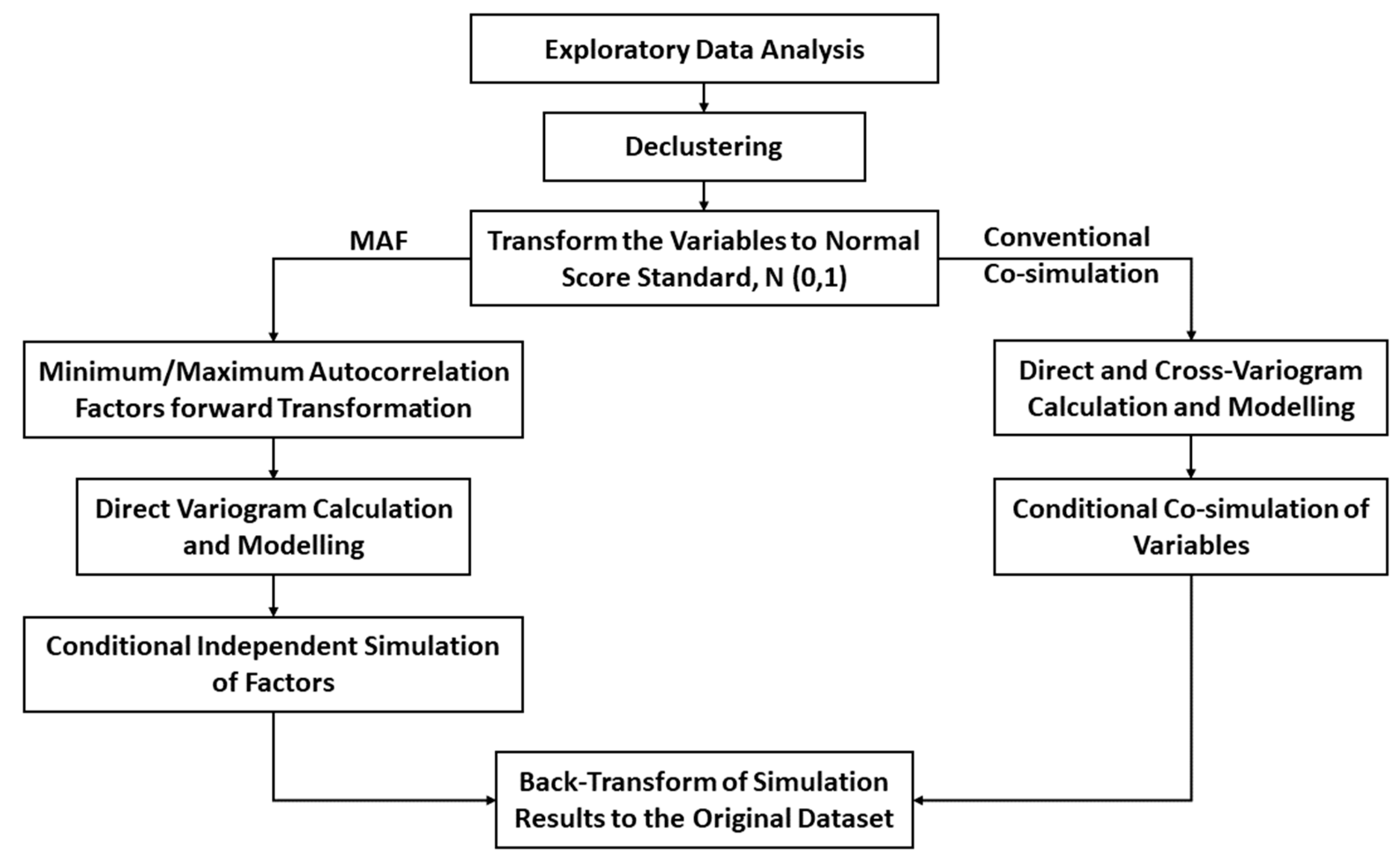
A brief illustration of both approaches is presented in Figure 2.
3. Application to an Actual Case study
The 2D dataset is composed of 3866 samples obtained from blast holes belonging to a porphyry copper deposit. The dataset is homotopic, means that the data are available for each variable at all sampling points [38]. Total copper (tCu) and soluble copper grades (sCu) have been measured at all sampling locations (the patterns are illustrated in Figure 3). As can be seen, the high-grade values are concentrated mostly in the northern part of the region. In the following subsection, the original values were multiplied by a constant scale factor in order to preserve the confidentiality of the dataset. Table 1 shows the statistical parameters obtained after applying the cell declustering [39]. The scarcity of data in some regions makes the sampling pattern irregular and statistical parameters possibly biased. The idea of declustering is to account for the weights of each location by the cell-based technique to correct the pseudo skewness in the global distribution of the dataset [33]. The low values of the coefficient of variation indicate that the data are well distributed in the region [40].
Multivariate analysis between these two variables by computing the linear correlation coefficient, explicitly means that those random attributes are highly correlated. This positive correlation also implies that total copper grade increases as the soluble copper grade increases and vice versa. Therefore, this characteristic motivates one to jointly estimate or simulate the total and soluble copper grades in the specified domain [37,41]. The reason is that, due to taking into account the global and local cross-correlation structure among the variables in joint spatial modeling, those algorithms are able to reproduce the underlying correlation measures at target locations after the process of modeling [38,42]. This spatial correlation can be introduced as direct and cross-variograms that are directly obtained from spatial continuity analysis [17]. However, as explained, the soluble copper grade is always less than or equal to the total copper grade (i.e., inequality constraint) (Figure 4) following a very sharp linear relationship, which makes the process of co-simulation difficult by conventional methodologies, since it is not able to preserve this restriction after the process of modeling. These restricted characteristics can be revealed through exploratory data analysis. Scatterplot as a qualitative examiner is a satisfactory tool to investigate the inequality constraint. Other exploratory data analysis approaches including the comparative statistics such as t-test and f-test can also be applied to compare the mean and variances of the populations, respectively. In the t-test, for instance, the hypothesis can be based on the inequality of the mean of the population between tCu and sCu. To come up with the problem of modeling of these two unequal variables, the original variables can be converted to new variables free of the inequality constraint. These new variables are taken into account in 3D spatial modeling and then need to be back-transformed to the original scales. These forward and backward transformations neutralize any absolute distortion might happen through the process of transformation. In this current study, the sCu is the only variable that can be converted to another variable, the so-called solubility ratio (SR) [7]. The tCu is kept unchanged and the process of modeling is implemented only by considering the new variable (SR) and unchanged variable (tCu). This conversion guarantees that the SR is always a proportion of sCu and consequently, the final model (i.e. after back-transformation) can precisely yield the relation of interest, sCu < tCu. The solubility ratio (SR) can be calculated by dividing the soluble copper grade by the total copper grade. As this value has no unit, it can be reported as a percentage:
3.1. Conventional Co-Simulation
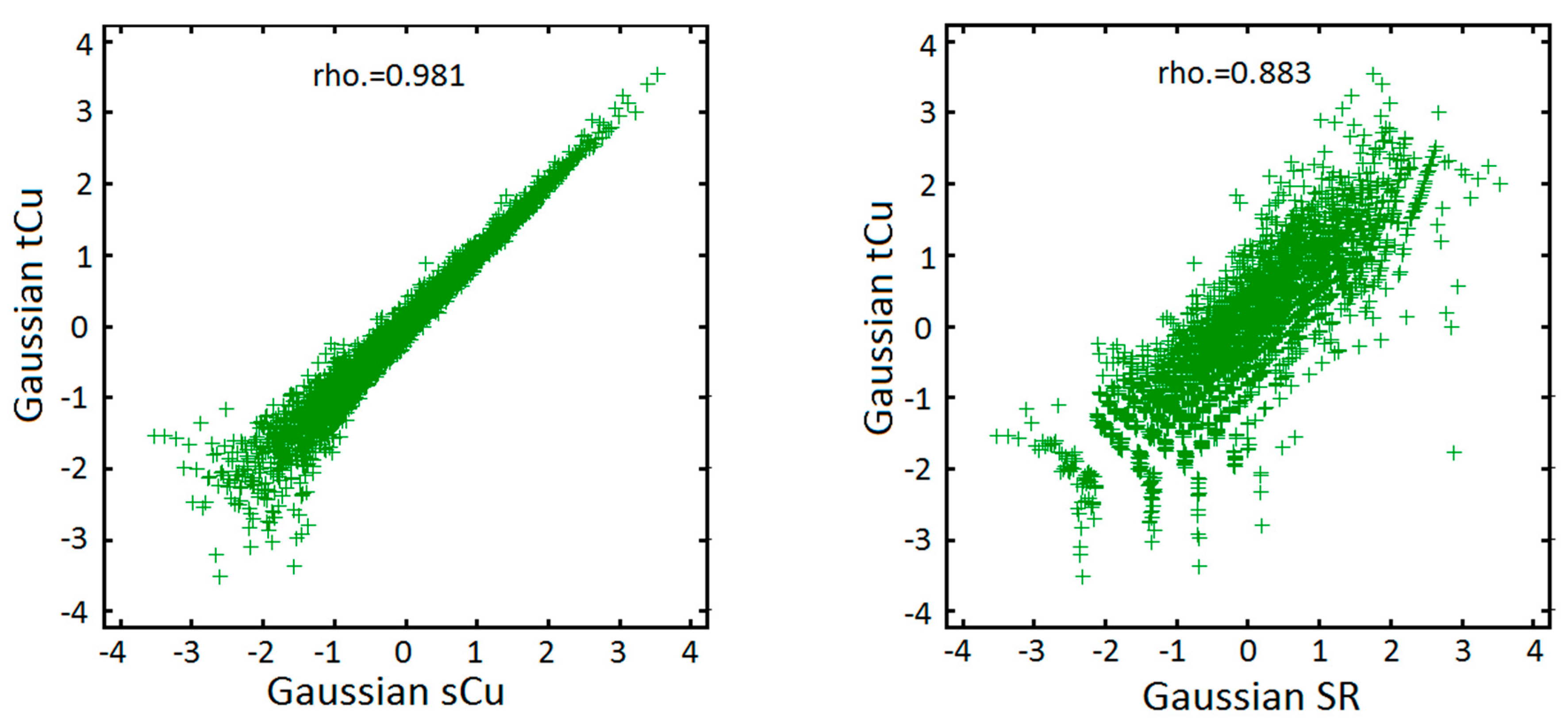
After converting the cross-correlated variables (tCu and sCu) into the variables free of the inequality constraint (tCu and SR), based on the following the steps explained in above section, it is of interest, to first co-simulate the total copper grade and solubility ratio by conventional Gaussian algorithm and then back transform them to the original scale (tCu and sCu). All the Gaussian simulation methodologies can be applied. However, turning bands co-simulation [41] has been employed in this study because of its versatility and straightforwardness [35]. Paravarzar et al. [35] showed that turning bands co-simulation algorithms outperform other Gaussian-based approaches such as sequential Gaussian co-simulation in terms of global and local statistical parameter reproduction and also in re-establishing the cross-correlation structures. Prior to the modeling, the converted variables are required to be transformed to the normal score values (Figure 5, right). This transformation guarantees that the values have standard Gaussian distribution and can be used in Gaussian simulation algorithms (Figure 6, right). It is worth mentioning that the scatter plot of normal scored original data without conversion to the new variables does not convey any multi-Gaussianity assumption, for which it restricts using the Gaussian simulation (Figure 6, left). Corroboration of multi-Gaussian assumption can be visually checked by elliptical shapes that appear in scatterplots of two transformed Gaussian random fields (Figure 6, right).
Co-simulation methodology requires that the spatial continuity is primarily modeled by calculation of direct and cross-variograms of the transformed variables. The experimental direct and cross-variograms should then be fitted by manual or semi-automatic fitting approaches [43,44] (Figure 7). In order to detect the anisotropy in the region, the variogram is calculated along different directions. Visual inspection showed that zonal and geometric anisotropies do not impact the spatial continuity measure and, consequently, the omni-directional variogram can be considered for describing the spatial variability in the region. Linear model of coregionalization (LMC) is then fitted consisting of two nested omni-directional spherical structures:
Linear model of coregionalization is widely applicable to fit such direct and cross-variograms, due to its mathematical simplicity [17,18,38]. The only restriction in LMC, is that the sill matrices should be positive semi-definite and the structures should be stationary permissible variogram models [44].
Having the fitted theoretical spatial continuity, turning bands co-simulation is then performed on a regular grid with dimension of 25 m × 10 m × 0.5 m. In this algorithm, it is of interest to stochastically simulate the cross-correlated variables (more than two). As a consequence, the cross-covariance function is needed to construct such a multi-dimensional Gaussian random field in the region. The non-conditional step is the same as tuning bands simulation for independent modeling of each variable; however, in part of the conditioning mechanism, simple co-kriging should be utilized for the process of conditioning to hard data (sampling locations). In this study, simple co-kriging is incorporated with a single searching strategy [45]. The proposed approaches can be substituted for ordinary co-kriging where the uncertainty is significant in terms of the mean value of the random field [7]. The type of neighborhood is moving with conditioning maximum up to 50, based on surrounding data characterized by isotropic distance equal 170 m derived from the variogram analysis. The number of lines for turning bands should be as large as possible [41]. Henceforth, it is set to 1000 lines for elimination of stripping effects and the number of realizations is considered to be 100.
3.2. Joint Simulation with MAF Transformation
The MAF factors are derived from the same normal score values explained in the conventional co-simulation section following the steps explained in the methodology section (i.e., Section 2.2). To do so, since in this study, data-driven MAF is used, it is necessary to consider an arbitrary lag separation distance except 0 for calculation of cross-correlation matrix; 10 m is chosen based on sampling spacing and range of spatial continuity. The MAF transformation matrix, which allows converting the Gaussian variables into factors, is the following:
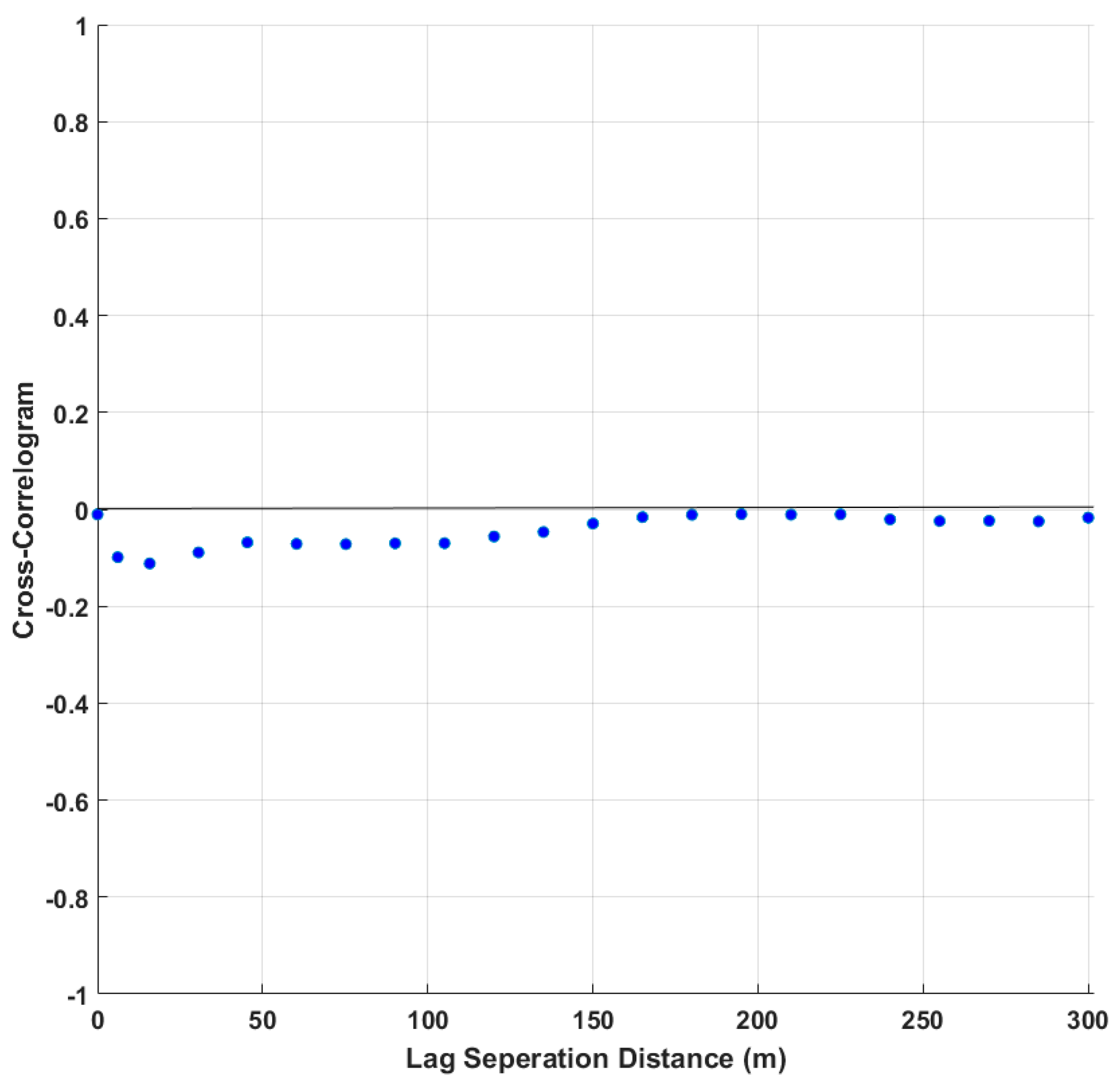
In order to check whether the factors are spatially decorrelated, a cross-correlogram was plotted. This shows that the spatial correlation between two factors and is close to zero (Figure 8), corroborating that the factors are effectively decorrelated at all lags. The histogram of the factors can also be checked to determine whether they follow the normal score distribution . Figure 9 shows the global distributions of the factors that follow a standard normal distribution.
Once the spatial decorrelation of factors is validated, the experimental direct variogram for each factor is computed and fitted:
The fitted model to each factor is two spherical structures. The spatial continuity direction is omni-directional, same as the one considered over previous normal score variables (Figure 10).
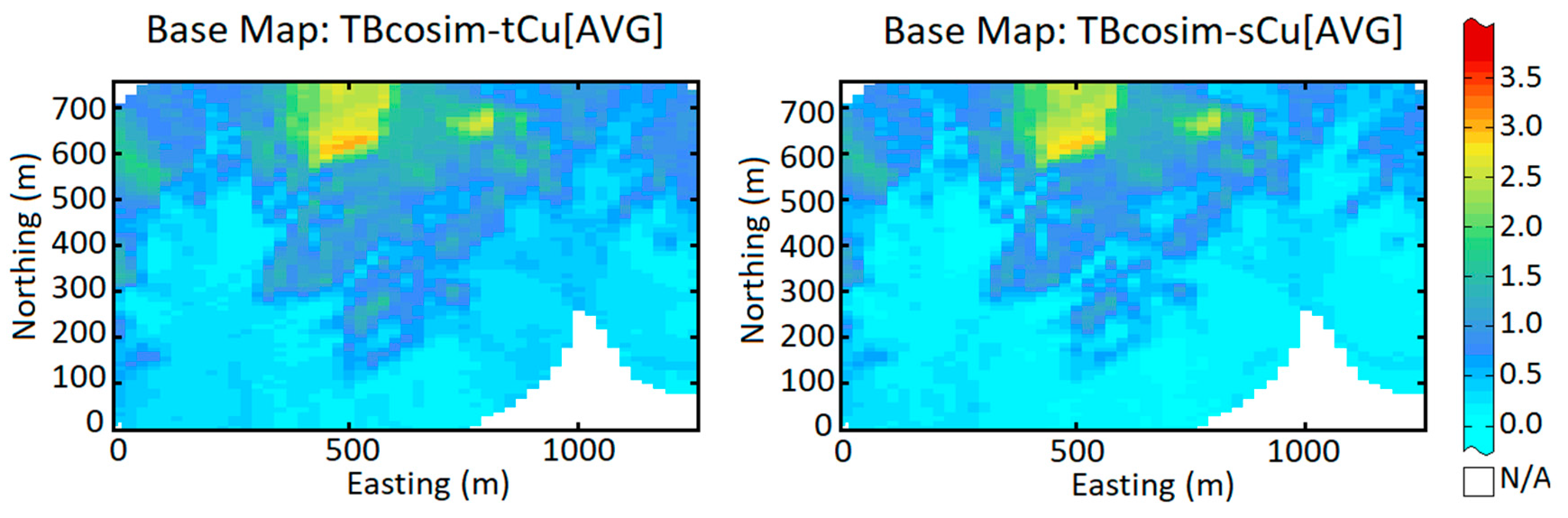
Having the fitted variogram structures over the factor and , the turning bands simulation algorithm [34] is employed to generate 100 realizations conditioned to two random fields of interest (factors). The size and dimension for independent simulation are the same as mentioned earlier for conventional Gaussian co-simulation. After simulation, it is necessary to back-transform the realization within two successive steps. The first back-transformation is from factor to normal score values by taking into account the inverse of matrix in Equation 10 and simply through its multiplication with the simulated factors; the second is from normal score values to total copper grade and solubility ratio. The latter uses the same function for transforming the total copper grade and solubility ratio to the normal score standard. This can be done by Gaussian anamorphosis functions [39] or quantile-quantile approach [36]. Since the aim of this research is to jointly simulate the total and soluble copper grades, the realizations so obtained are then back-converted by Equation 8 to desired space. The maps of the average of 100 realizations (E-type) produced from both methods: conventional co-simulation and joint simulation with MAF, are illustrated in Figure 11 and Figure 12.
3.3. Validation of Results
In this section, it is of interest to validate the results of simulation realization produced by two underlying methodologies (TBCOSIM considering the linear model of coregionalization and MAF). The criteria for such an examination are the statistical parameter of the original dataset that are spatially declsutered and that effectively, the outputs of two models can be compared with. For this purpose, the tests are carried out on the basis of two families. The first family aims at comparing the global statistical parameters of the derived realizations to the declustered raw variables. In this context, reproduction of global mean, variance and correlation is considered. The second family corresponds to checking the spatial reproduction of local continuity by applying the variogram analysis over the produced realizations. A variogram is a good measure of spatial variability for quantification of dissimilarity between data pairs in a region [39,42]. This can be a good tool for calculation of local variability.
3.3.1. Validation of Global Statistical Parameter
The first examination consists of analyzing the mean and variance reproductions of simulation realization for both TBCOSIM and MAF approaches, in order to compare with the original declustered means of total and soluble copper grades. Although the mean values are the acceptable measure for comparison of realizations, even with same central value, the simulation results might show absolutely different distributions. The variance as an additional measure of variation is required for better interpretation of the data dispersion. Consequently, the mean and variance are calculated over each realization. The average of those mean and variance values over 100 realizations are presented in Table 2. As can be seen, the reproduction of the mean is dramatically adequate for two variables, whereas the reproduction of variance is good and slightly higher compared to the input declustered variance. This minor difference can be interpreted due to the influence of conditioning data. The simulation results before back-transformation for SR and tCu are also checked thoroughly to examine whether the realizations follow a normal standard distribution.
The strength of the relationship between variables can be quantified through correlation coefficients. In order to measure the interrelation characteristics between the total and soluble copper grades, the correlation coefficient is calculated taking into account all the realizations. The average correlation computed value over 100 realizations is obtained from MAF and TBCOSIM (. A comparison to the declustered original correlation coefficient indicates that not only is the LMC is sufficient for re-establishing the data cross correlation, the proposed algorithm (joint simulation with MAF) is also capable of yielding the desired correlation (Table 2).
Figure 13 shows the scatter plot between these two variables before and after modeling. The shape of the bivariate relationship (dependency) between total and soluble copper grades and also the inequality constraint are satisfactorily reproduced. These results imply that the proposed algorithm does not show loss of accuracy.
3.3.2. Validation of Local Statistical Parameter
Another way to quality check simulation results is to check the spatial continuity. In this respect, direct and cross-variograms of the simulated realizations should be compared with the fitted theoretical model [16]. Figure 14 shows the comparison of the direct and cross experimental variogram of simulations obtained from TBCOSIM and MAF approaches with the variogram model computed from original declustered variables. In all cases, the spatial continuity has been sufficiently reproduced. However, a slight difference appeared between average variogram of the simulation results (dashed red line) and theoretical variogram (solid blue line), because of the impact of conditioning sample points that distorts the prior model and also the restriction in the size of a domain [41,46,47]. One solution to avoid such a contrast is to use non-conditional simulation which is not in the scope of this study. However, the non-conditional simulation is only applicable for validation of statistical parameters and is not suitable for further analysis and decision-making in a project.
Another measure for evaluation of spatial continuity is the codispersion function based on the correlation coefficient between lag separation increments. This function for tCu and sCu is given by [39]:
The codispersion function is computed over the simulation results obtained from the TBCOSIM and MAF algorithm and is then compared with both of the original codispersion functions calculated from original declustered dataset (Figure 15). The trend of those curves corroborate that the spatial correlation between lag separation increments is independent of the increase in the lag itself. This type of characteristic can be revealed through visual inspection of the graphs, as long as two algorithms follow the same features (gray and red lines) compared with the original codipersion function (blue line). However, similar to variogram reproduction, slight deviation of simulation results is due to the influence of conditioning data.
3.3.3. Sensitivity Analysis of the Number of Simulations
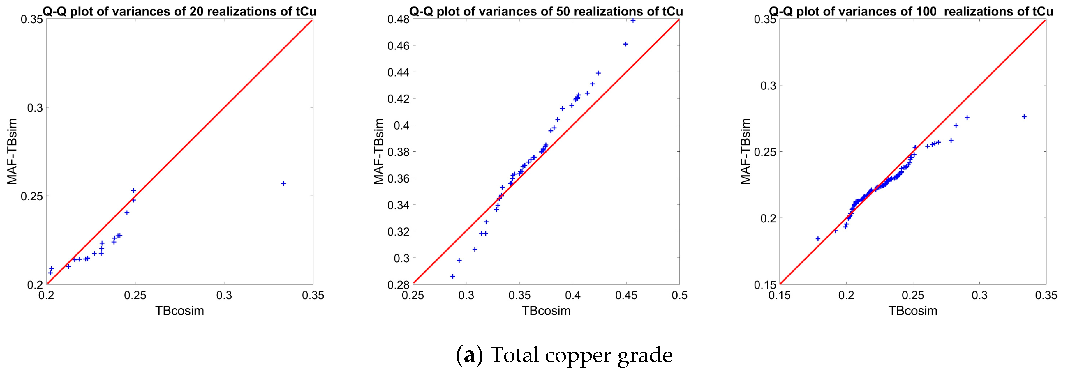
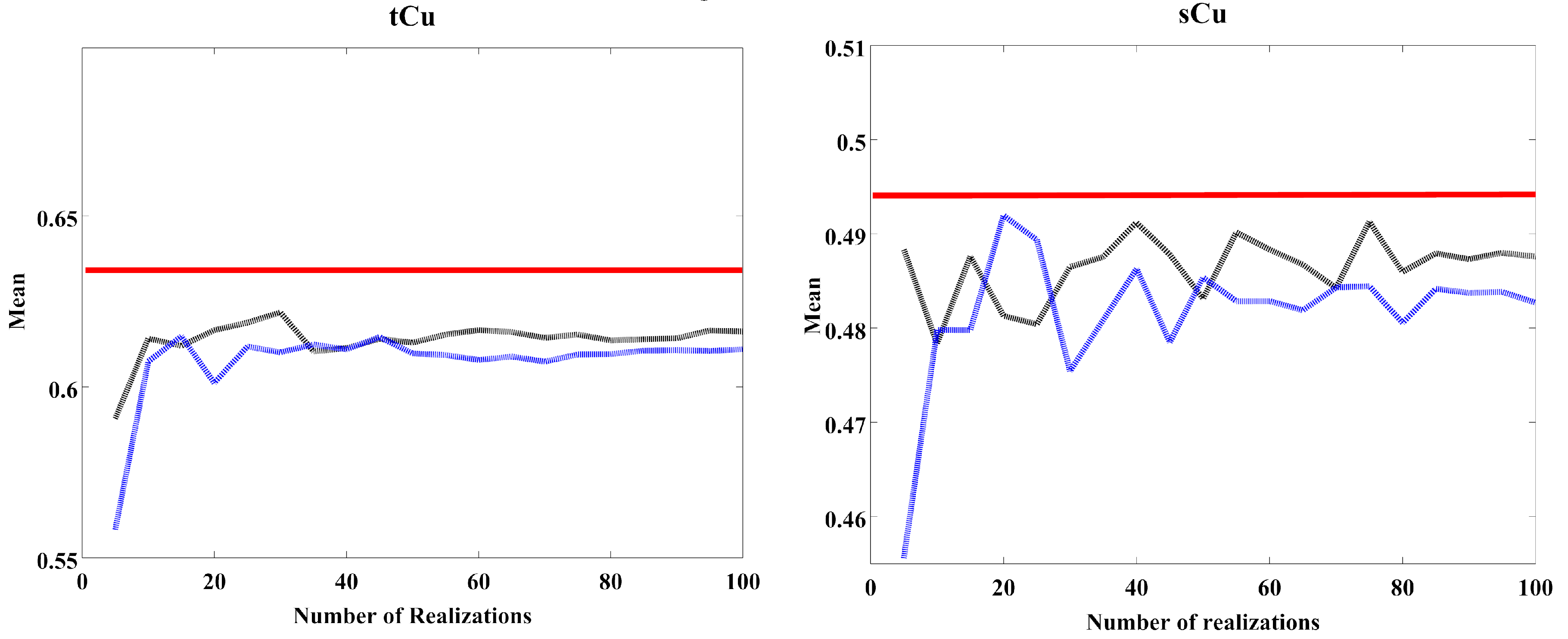
The concept of simulation is to produce a large number of realizations to quantify the uncertainty at target locations [40,48]. However, finding the adequate number of realizations is still a meaningful question in geostatistical modeling of the variables [49]. In this section, it is of interest to perform a sensitivity analysis over the number of realizations. The test here is to compare the distributions of the mean values and variances calculated over different numbers of realizations. To do so, three realizations (20, 50 and 100) are considered. In each case, the mean and variance of each realization are calculated and the relevant distributions are subsequently deduced and compared with each other. For instance, in the case of 20 realizations, through Quantile-Quantile plot (QQ-plot) analysis, 20 values of the mean and 20 values of the variance are obtained from TBCOSIM (as the reference) and the underlying distribution is compared with the 20 values of the mean and 20 values of the variance that are computed from MAF results. The QQ-plot can be interpreted as follow [50]: a) when all the points on a QQ-plot fall long the diagonal line, the two distributions are exactly the same; b) a systematic departure above or below the diagonal line indicates that the mean value of the two underlying distributions is different; c) a slope different from the diagonal indicates that the variance of the two distributions is different; d) curvature on a QQ-plot indicates that the two distributions have different shapes. As can be seen from Figure 16 and Figure 17, the distribution of mean and variance values approach the diagonal line by increasing the number of realizations from 20 to 100. This is worse when one considers small numbers of realizations (e.g., 20) that lead to a systematic departure from the diagonal line, indicating the significant difference in two distributions obtained from TBCOSIM and MAF. The results also showed that 100 realizations can be considered as an acceptable number of realizations for the MAF analysis for reproduction of the desired uncertainty that can be expected from TBCOSIM.
The presented Q-Q plots show the reproduced global distribution of the simulation results. In order to check the sensitivity of variability of mean values versus the number of realizations, 20 groups of cases including {5, 10, 15… 100} realizations are considered for this type of examination. Figure 18 shows that the variability for both algorithms, MAF and TBCOSIM (blue and black lines, respectively) following very close trends in both tCu and sCu variables compared to the original declustered mean (red line). Slight deviation of mean values from the original declustered mean is due to the influence of conditioning data. It is also worth mentioning that based on Figure 18, the fluctuations after approximately 30 realizations stabilize in terms of convergence to the declustered original mean. However, the convergence to the original global distribution is more satisfying whenever one considers 100 realizations (Figure 17).
3.3.4. Post Processing the Realizations: Probabilistic Domaining of Geometallurgical Domains
Having the result of realizations, one is able to take them into account for further decision-making process in a mining project. An advantageous aspect of this act is to define the possible destination of a mined block for mineral processing plants. Since the uncertainty is estimated through the output of simulation approaches, the probabilistic areas of the underlying mineral processing destinations such as flotation, leaching and dump plants can be identified, in which they show a measure of confidence to decide about the destination of that block of interest. In this respect, the areas with these characteristics can be considered as the geometallurgical domains. In this oxide copper deposit, each mined block can have three possible destinations: flotation plant provided that total copper grade is above 0.4% and solubility ratio is less than 70%, leaching plant provided that total copper grade is above 0.4% and solubility ratio is more than 70% and dump otherwise. Figure 19 shows the probable areas of both leaching and flotation plants obtained from post processing the 100 simulation results produced by MAF approach. Construction of those probability maps is based on the calculation of the frequency of occurrence of each geometallurgical domain over 100 conditional realizations. They show the risk of finding a geometallurgical domain different from others. The sectors with little uncertainty are those associated with a high probability for a given geometallurgical domain (colored in red in Figure 19), indicating that there is a little risk of not finding this geometallurgical domain, or those associated with a very low probability (colored in blue in Figure 19), indicating that one is quite sure of not finding this domain, while the other sectors (colored in light blue, green or yellow in Figure 19) are more uncertain. However, those descriptions are probabilistic and not deterministic.
3.3.5. Validation against Actual Data
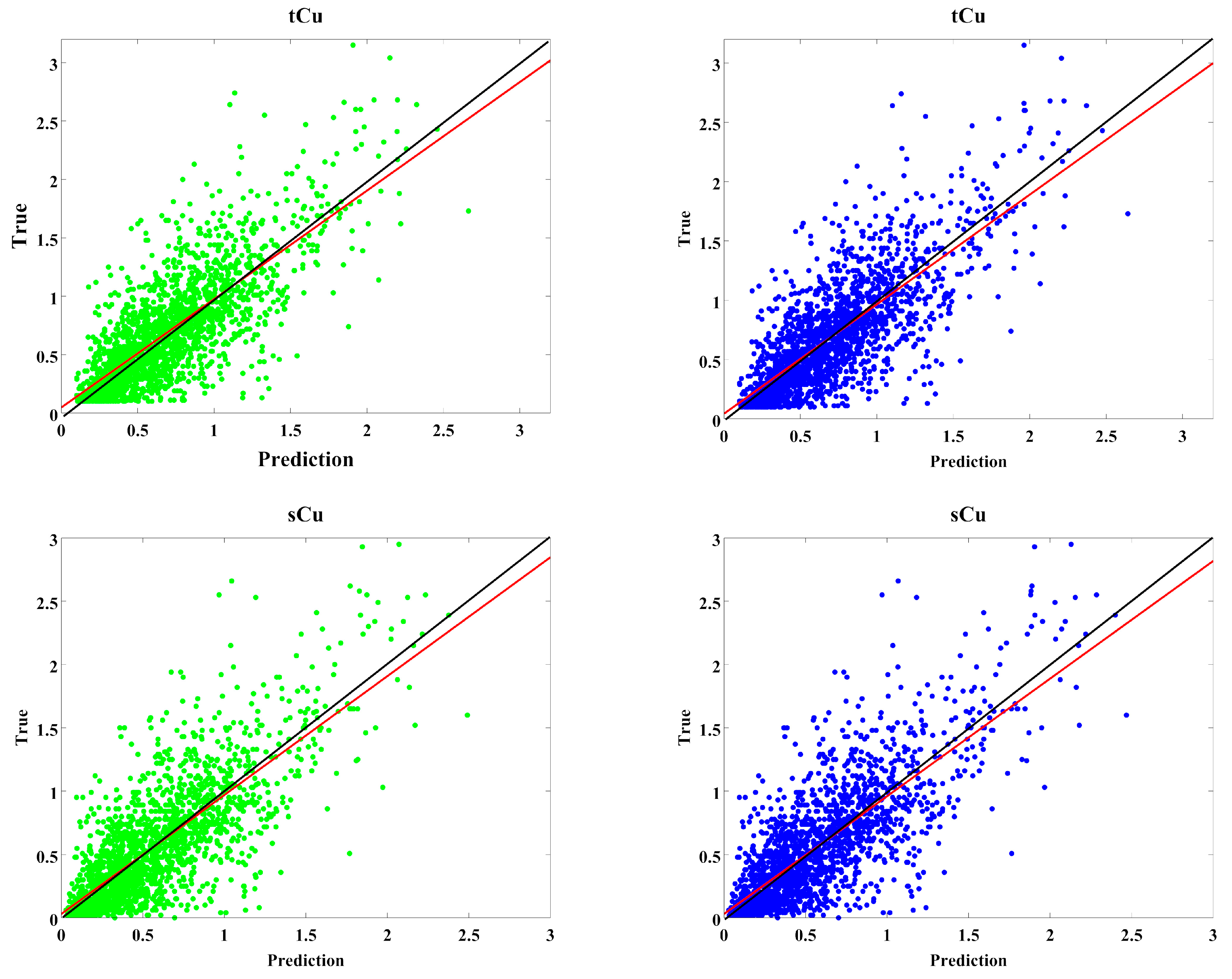
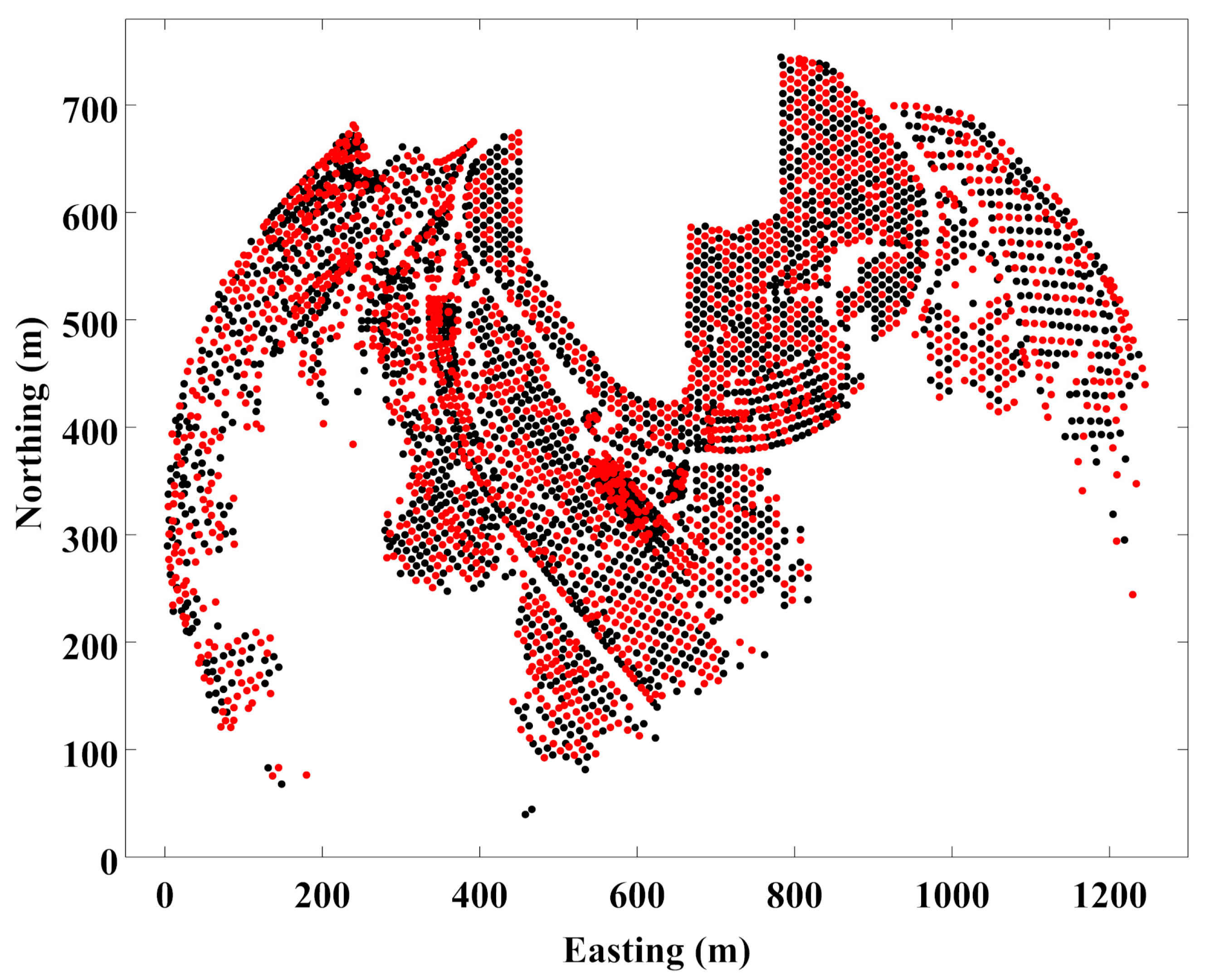
The produced model can also be examined versus the actual value of underlying attributes, that is, mostly based on production data, in which the true values are known after extraction of the simulated block. In this study, the production data are not available. Henceforth, in order to assess the proficiency of the simulation results, a typical validation technique, which is suitable for validation of geostatistical algorithms, is taken into account for both underlying variables, tCu and sCu. This test, the so-called jackknife approach, aims at resampling without replacement when alternative data values are re-estimated from other non-overlapping data sets [35]. This type of analysis is basically applicable for evaluation of the variogram model, type of kriging and the search strategy in geostatistical contexts. Nevertheless, the jackknife approach can also be applicable for evaluation of simulation results. To implement this examination technique, the underlying dataset in this study, consisting of 3866 sample points, was divided randomly into two parts. One set of data is considered as analysis and another non-overlapping set of data is chosen as test (Figure 20). The analysis data set is then incorporated to simulate the tCu and sCu at sample locations of test data. To do so, turning bands co-simulation and the proposed algorithm in this study (MAF) are applied following the procedures, which are thoroughly discussed in previous sections. Since the true values of tCu and sCu are known at test sample locations, the average of simulation results in the same locations conditioned to the analysis dataset can provide the prediction values of tCu and sCu at those corresponding locations. Therefore, a scatter plot can be drawn though the test sample points, wherever two sorts of data are available: true and predicted measures of tCu and sCu. The results are depicted in Figure 21, and the bivariate distribution of points and their tendency to the diagonal line (black line) reveal that both approaches provide analogous outputs and one is able to use MAF, rather than a co-simulation approach without loss of generality, in the case when dealing with possible actual data (i.e. production data) is significant.
Scatterplot between prediction and true values, somehow provide the visual inspection, mostly qualitative for examination of proficiency of the geostatistical algorithms. One quantitative measure can be relative error which is the ratio of the value of the difference of an estimated value and an actual value compared to the actual value:
The mean of relative errors in both approaches (MAF and TBCOSIM) for two variables, tCu and sCu are very close to each other and also close to zero (Table 3), indicating that not only the simulated results for prediction of actual data are trustworthy, both techniques produced the tight results in what concerns the error computation.
4. Discussion on Application and Limitations of the Proposed Approach
This study showed that the use of LMC can be eliminated in order to build a simpler geometallurgical model through the factorization approach, in the case whenever the inequality constraint exists among the variables, which significantly requires less computational time and resources. In addition to this benefit for removing this spatial continuity inference step in LMC, another advantage is substituting the co-kriging for kriging in the proposed algorithm that is less demanding and considerably accelerates the process of modeling, in the particular case wherever there are plenty of data and sample points. It is also worth mentioning that, although the proposed algorithm is not an offshoot of conventional co-simulation, it gives the same benefit in preserving the spatial continuity structures of the dataset. Besides those advantageous, there are some areas of research that can be proposed for future work of some cases which may restrict using the proposed algorithm for the time being. For instance, there are situations where the total copper grade is more available than soluble copper grade, implying a heterotopic sampling pattern. In this situation, although a “change of variable” technique is suitable, the joint simulation step by MAF is not adequate because of its restriction into the homotopic sampling pattern. Another issue that can be discovered is related to the number of structures in the linear model of coregionalization. The MAF technique is limited to two structures in variogram analysis. More advanced techniques such as Enhanced Coregionalization Analysis [51] can be proposed instead. A related point when considering the validation technique against actual data is that the jackknife approach applied here is about the simulation data. The model can also be validated through reconciliation and availability of actual data from a mining site.
5. Conclusions
Geostatistical modeling has been widely used in spatial modeling of geometallurgical variables. However, since those variables have inherent complex characteristics such as the inequality constraint, one needs to consider the improved methodologies. In this study, a new algorithm is proposed to jointly simulate total and soluble copper grades with inequality constraint. In order to show the versatility of the presented technique, the results are compared with those obtained from conventional co-simulation that is based on using the linear model of coregionalization (LMC). A case study from a copper deposit consisting of total and soluble copper grades, with homotopic sampling was carried out. In order to circumvent the problem of inequality constraint modeling, the “change of variable” technique is taken into account to compute a new variable, namely, the solubility ratio (SR). This new variable, SR, and total copper grade (tCu) are then taken into account for the process of modeling by the proposed algorithm. The simulated results of SR and tCu are then back-transformed to the original scales, tCu and sCu. The turning bands co-simulation is also applied as a benchmark to compare the outputs of the proposed algorithm. Global and local statistical analysis, such as examination of mean, variance and variogram reproduction, showed quite satisfactory results. The results also approved that the correlation coefficients between total and soluble copper for both algorithms (conventional co-simulation and proposed algorithm (MAF)) are reproduced effectively, and multivariate complex interrelation of variables is regenerated without any deviation from the primary inequality constraint. In addition, the results of the proposed algorithm for joint simulation with MAF show similar results as in co-simulation. In order to show the application of simulation results, the realizations are post–processed to quantify the probabilistic destination of geometallurgical domains (e.g. dump, flotation and leaching plant). Those maps are appropriate for further analysis of a mining project such as mine design and geometallurgical plant studies.
Author Contributions
Y.A. designed and conducted the experiments, Y.A. and N.M. wrote the paper and reviewed the results and E.T. reviewed the results and the paper.
Acknowledgments
The first and second authors acknowledge the Nazarbayev University for supporting this work via “Faculty Development Competitive Research Grants for 2018–2020” under Grant Contract No. 090118FD5336. The corresponding author is thankful to the University of Chile for providing the dataset. The two anonymous reviewers and the Editor are also thanked for their constructive comments which substantially improved the overall quality of the paper.
Conflicts of Interest
The authors declare no conflict of interest. The founding sponsors had no role in the design of the study; in the collection, analyses, or interpretation of data; in the writing of the manuscript, and in the decision to publish the results.
References
- Macfarlane, A.S.; Williams, T.P. Optimizing value on a copper mine by adopting a geometallurgical solution. J. South. Afr. Inst. Min. Metall. 2014, 114, 929–935. [Google Scholar]
- Almeida, J.A. Modelling of cement raw material compositional indices with direct sequential cosimulation. Eng. Geol. 2010, 114, 26–33. [Google Scholar] [CrossRef]
- Tercan, A.E.; Sohrabian, B. Multivariate geostatistical simulation of coal quality by independent components. Int. J. Coal Geol. 2013, 112, 53–66. [Google Scholar] [CrossRef]
- Brissette, M.; Mihajlovic, V.; Sanuri, S. Geometallurgy: New accurate test work to meet required accuracies of mining project development. In Proceedings of the XXVII International Mineral Processing Congress, Santiago, Chile, 20–24 October 2014. [Google Scholar]
- Deutsch, J.L.; Szymanski, J.; Etsell, T.H. Metallurgical Variable Re-expression for Geostatistics. In Geostatistical and Geospatial Approaches for the Characterization of Natural Resources in the Environment; Springer: Cham, Switzerland, 2016; pp. 83–88. [Google Scholar]
- Tolosana-Delgado, R.; Mueller, U.; van den Boogaart, K.G.; Ward, C.; Gutzmer, J. Improving processing by adaption to conditional geostatistical simulation of block compositions. J. South. Afr. Inst. Min. Metall. 2015, 115, 13–26. [Google Scholar] [CrossRef] [Green Version]
- Emery, X. Co-simulating total and soluble copper grades in an oxide ore deposit. Math. Geosci. 2012, 44, 27–46. [Google Scholar] [CrossRef]
- Hosseini, S.A.; Asghari, O. Simulation of geometallurgical variables through stepwise conditional transformation in Sungun copper deposit, Iran. Arab. J. Geosci. 2015, 8, 3821–3831. [Google Scholar] [CrossRef]
- Bai, S.; Fu, X.; Li, C.; Wen, S. Process improvement and kinetic study on copper leaching from low-grade cuprite ores. Physicochem. Probl. Miner. Process 2018, 54, 300–310. [Google Scholar]
- Pizarro, S.; Emery, X. Geostatistical joint modelling of total and soluble copper grades. In Proceedings of the 2nd International Seminar on Geology for the Mining Industry GEOMIN 2011, Antofagasta, Chile, 8–10 June 2011; Beniscelli, J., Kuyvenhoven, R., Hoal, K.O., Eds.; Gecamin Ltda: Santiago, Chile, 2011. [Google Scholar]
- Cáceres, A.; Riquelme, R.; Emery, X.; Díaz, J.; Fuster, G. Total and soluble copper grade estimation using minimum/maximum autocorrelation factors and multigaussian kriging. In Proceedings of the 2nd International Seminar on Geology for the Mining Industry GEOMIN 2011, Antofagasta, Chile, 8–10 June 2011; Beniscelli, J., Kuyvenhoven, R., Hoal, K.O., Eds.; Gecamin Ltda: Santiago, Chile, 2011. [Google Scholar]
- Lange, W.; Emery, X. Joint simulation of total and soluble copper grades in an oxide copper deposit. In Proceedings of the 5th International Conference on Innovation in Mine Operations, Santiago, Chile, 20–22 June 2012; Kuyvenhoven, R., Morales, J.E., Vega, C., Eds.; Gecamin Ltda: Santiago, Chile, 2012; pp. 62–63. [Google Scholar]
- Dubrule, O.; Kostov, C. An interpolation method taking into account inequality constraints: I. Methodology. Math. Geol. 1986, 18, 33–51. [Google Scholar] [CrossRef]
- Leuangthong, O.; Deutsch, C.V. Stepwise conditional transformation for simulation of multiple variables. Math. Geol. 2003, 35, 155–173. [Google Scholar] [CrossRef]
- Abildin, Y.; Madani, N.; Topal, E. Geostatistical Modelling of Geometallurgical Variables through Turning Bands Approach. In Proceedings of the 25th World Mining Congress, Astana, Kazakhstan (WMC 2018), Astana, Kazakhstan, 19–22 June 2018. [Google Scholar]
- Emery, X. Testing the correctness of the sequential algorithm for simulating Gaussian random fields. Stoch. Environ. Res. Risk Assess. 2004, 18, 401–413. [Google Scholar] [CrossRef]
- Journel, A.G.; Huijbregts, C.J. Mining Geostatistics; Academic Press: Cambridge, MA, USA, 1978. [Google Scholar]
- Goovaerts, P. Spatial orthogonality of the principal components computed from coregionalized variables. Math. Geol. 1993, 25, 281–302. [Google Scholar] [CrossRef]
- Bandarian, E.M.; Bloom, L.M.; Mueller, U.A. Direct minimum/maximum autocorrelation factors within the framework of a two structure linear model of coregionalisation. Comput. Geosci. 2008, 34, 190–200. [Google Scholar] [CrossRef]
- Switzer, P.; Green, A.A. Min/max autocorrelation factors for multivariate spatial imagery. Comput. Sci. Stat. 1985, 16, 13–16. [Google Scholar]
- Maleki, M.; Madani, N. Multivariate Geostatistical Analysis: An application to ore body evaluation. Iran. J. Earth Sci. 2017, 8, 173–184. [Google Scholar]
- Kim, H.J.; Song, Y.; Lee, K.H. Inequality constraint in least-squares inversion of geophysical data. Earth Planets Space 1999, 51, 255–259. [Google Scholar] [CrossRef] [Green Version]
- Abrahamsen, P.; Benth, F.E. Kriging with Inequality Constraints. Math. Geol. 2001, 33, 719–744. [Google Scholar] [CrossRef]
- Journel, A.G. Constrained interpolation and qualitative information—The soft kriging approach. Math. Geol. 1986, 18, 269–286. [Google Scholar] [CrossRef]
- Vargas-Guzmán, J.A.; Dimitrakopoulos, R. Successive nonparametric estimation of conditional distributions. Math. Geol. 2003, 35, 39–52. [Google Scholar] [CrossRef]
- Tran, T.T.; Murphy, M.; Glacken, I. Semivariogram structures used in multivariate conditional simulation via minimum/maximum autocorrelation factors. In Proceedings of the XI International Congress, IAMG, Liège, Belgium, 3–8 September 2006. [Google Scholar]
- Davis, B.M.; Greenes, K.A. Estimation using spatially distributed multivariate data: An example with coal quality. J. Int. Assoc. Math. Geol. 1983, 15, 287–300. [Google Scholar] [CrossRef]
- Suro-Perez, V.; Journel, A.G. Indicator principal component kriging. Math. Geol. 1991, 23, 759–788. [Google Scholar] [CrossRef]
- Rondon, O. Teaching aid: Minimum/maximum autocorrelation factors for joint simulation of attributes. Math. Geosci. 2012, 44, 469–504. [Google Scholar] [CrossRef]
- Desbarats, A.J. Geostatistical modeling of regionalized grain-size distributions using min/max autocorrelation factors. In geoENV III—Geostatistics for Environmental Applications; Springer: Dordrecht, The Netherlands, 2001; pp. 441–452. [Google Scholar]
- Desbarats, A.J.; Dimitrakopoulos, R. Geostatistical simulation of regionalized pore-size distributions using min/max autocorrelation factors. Math. Geol. 2000, 32, 919–942. [Google Scholar] [CrossRef]
- Rivoirard, J. Introduction to Disjunctive Kriging and Non-Linear Geostatistics; No. 551.021 R626i; Oxford University Press: Oxford, UK, 1994. [Google Scholar]
- Deutsch, C.V.; Journel, A.G. GSLIB: Geostatistical Software Library and User’s Guide, 2nd ed.; Oxford University Press: New York, NY, USA, 1998. [Google Scholar]
- Emery, X.; Lantuéjoul, C. Tbsim: A computer program for conditional simulation of three-dimensional gaussian random fields via the turning bands method. Comput. Geosci. 2006, 32, 1615–1628. [Google Scholar] [CrossRef]
- Paravarzar, S.; Emery, X.; Madani, N. Comparing sequential Gaussian and turning bands algorithms for cosimulating grades in multi-element deposits. Comptes Rendus Geosci. 2015, 347, 84–93. [Google Scholar] [CrossRef]
- Madani, N.; Ortiz, J. Geostatistical Simulation of Cross-Correlated Variables: A Case Study through Cerro Matoso Nickel-Laterite Deposit. In Proceedings of the 26th International Symposium on Mine Planning and Equipment Selection, Luleå, Sweden, 29–31 August 2017. [Google Scholar]
- Eze, P.N.; Madani, N.; Adoko, A.C. Multivariate Mapping of Heavy Metals Spatial Contamination in a Cu–Ni Exploration Field (Botswana) Using Turning Bands Co-simulation Algorithm. Nat. Resour. Res. 2018, 1–16. [Google Scholar] [CrossRef] [Green Version]
- Wackernagel, H. Multivariate Geostatistics: An Introduction with Applications; Springer: Berlin/Heidelberg, Germany, 2003. [Google Scholar]
- Goovaerts, P. Geostatistics for Natural Resources Evaluation; Oxford University Press: New York, NY, USA, 1997. [Google Scholar]
- Rossi, M.; Deutsch, C.V. Mineral Resource Estimation; Springer: New York, NY, USA, 2014. [Google Scholar]
- Emery, X. A turning bands program for conditional co-simulation of cross-correlated Gaussian random fields. Comput. Geosci. 2008, 34, 1850–1862. [Google Scholar] [CrossRef]
- Chilès, J.P.; Delfiner, P. Geostatistics: Modeling Spatial Uncertainty; Wiley: New York, NY, USA, 2012. [Google Scholar]
- Goulard, M.; Voltz, M. Linear corregionalization model: Tools for estimation and choice of cross variogram matrix. Math. Geol. 1992, 30, 589–615. [Google Scholar]
- Emery, X. Iterative algorithms for fitting a linear model of coregionalization. Comput. Geosci. 2010, 36, 1150–1160. [Google Scholar] [CrossRef]
- Madani, N.; Emery, X. A comparison of search strategies to design the cokriging neighborhood for predicting coregionalized variables. Stoch. Environ. Res. Risk Assess. 2018, 1–17. [Google Scholar] [CrossRef]
- Lantuejoul, C. Geostatistical Simulation, Models and Algorithms; Springer: Berlin/Heidelberg, Germany, 2002; p. 256. [Google Scholar]
- Emery, X. Conditioning simulations of Gaussian random fields by ordinary kriging. Math. Geol. 2007, 39, 607–623. [Google Scholar] [CrossRef]
- Deutsch, C.V. All Realizations All the Time. In Handbook of Mathematical Geosciences; Daya Sagar, B., Cheng, Q., Agterberg, F., Eds.; Springer: Cham, Switzerland, 2018. [Google Scholar]
- Jakab, N. Stochastic modeling in geology: Determining the sufficient number of models. Central Eur. Geol. 2017, 60, 135–151. [Google Scholar] [CrossRef] [Green Version]
- Pyrcz, M.; Deutsch, C.V. Geostatistical Reservoir Modeling; Oxford University Press: New York, NY, USA, 2014. [Google Scholar]
- Emery, X.; Ortiz, J.M. Enhanced coregionalization analysis for simulating vector Gaussian random fields. Comput. Geosci. 2012, 42, 126–135. [Google Scholar] [CrossRef]
Figure 1.
Different settings of inequality constraint in a dataset with their marginal distributions; and : the underlying variables, (a): unequal variables with the same distribution and linear relationship, (b): unequal variables with a different distribution linear relationship, (c): unequal variables with different distributions and non-linear relationship.

Figure 2.
Graphic flowchart for both approaches (MAF and Conventional co-simulation).

Figure 3.
Base map for the location of samples in the plane (the coordinates are local). (a) Total copper grade (tCu); (b) Soluble copper grade (sCu).
Figure 3.
Base map for the location of samples in the plane (the coordinates are local). (a) Total copper grade (tCu); (b) Soluble copper grade (sCu).
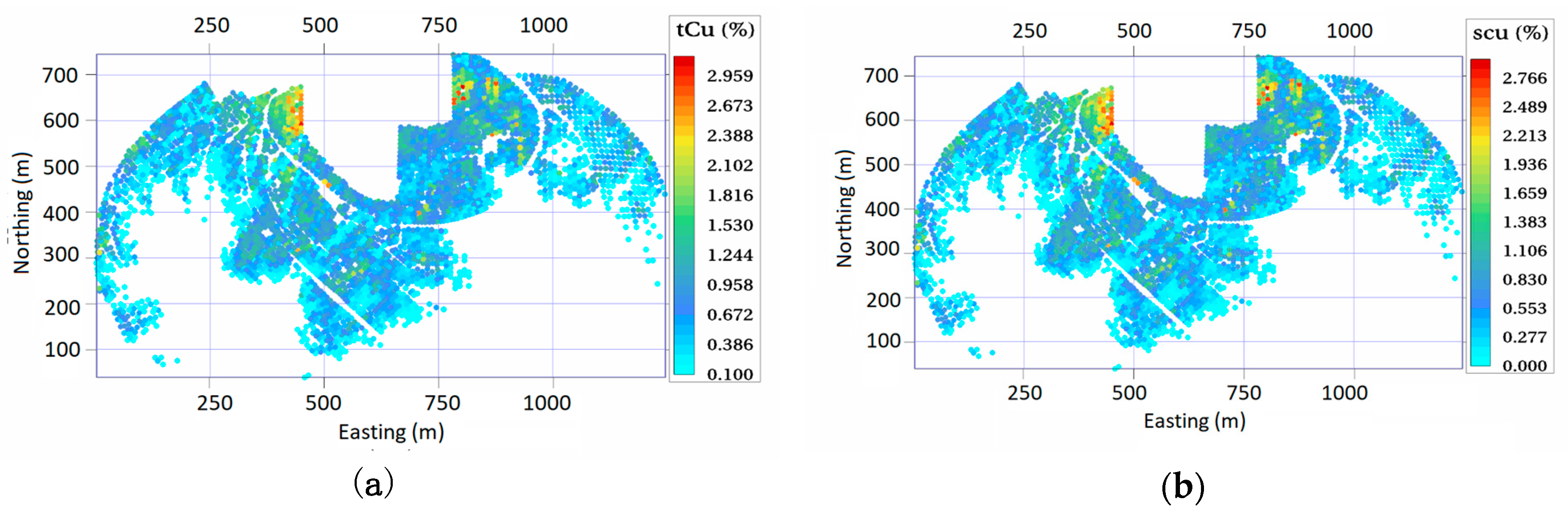
Figure 4.
Scatterplot between total and soluble copper grades.
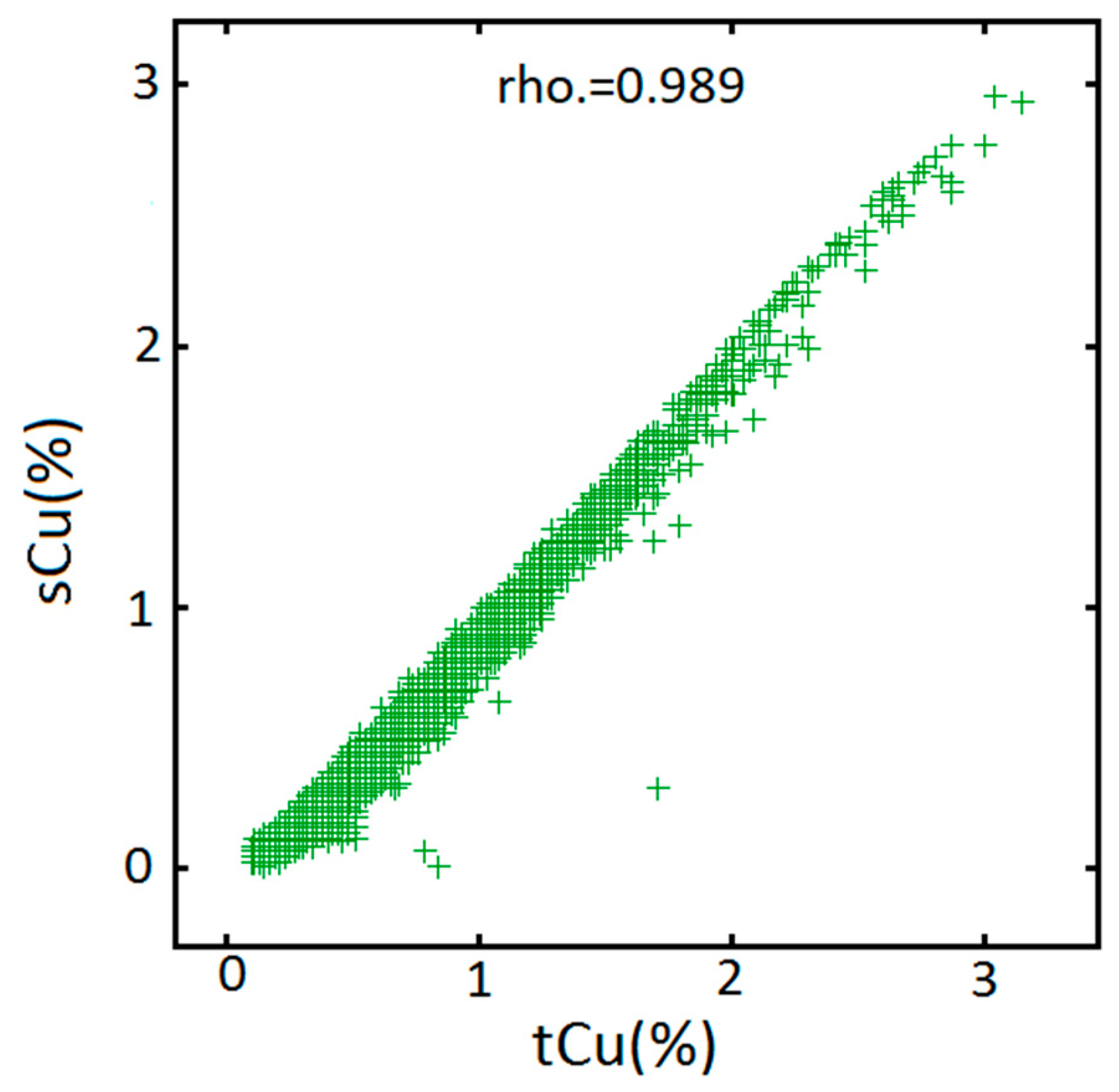
Figure 5.
Normal score transformation (left: declustered histogram of the original data and right: histogram of the normal score values.
Figure 5.
Normal score transformation (left: declustered histogram of the original data and right: histogram of the normal score values.

Figure 6.
Scatter plot of the data before and after conversion.

Figure 7.
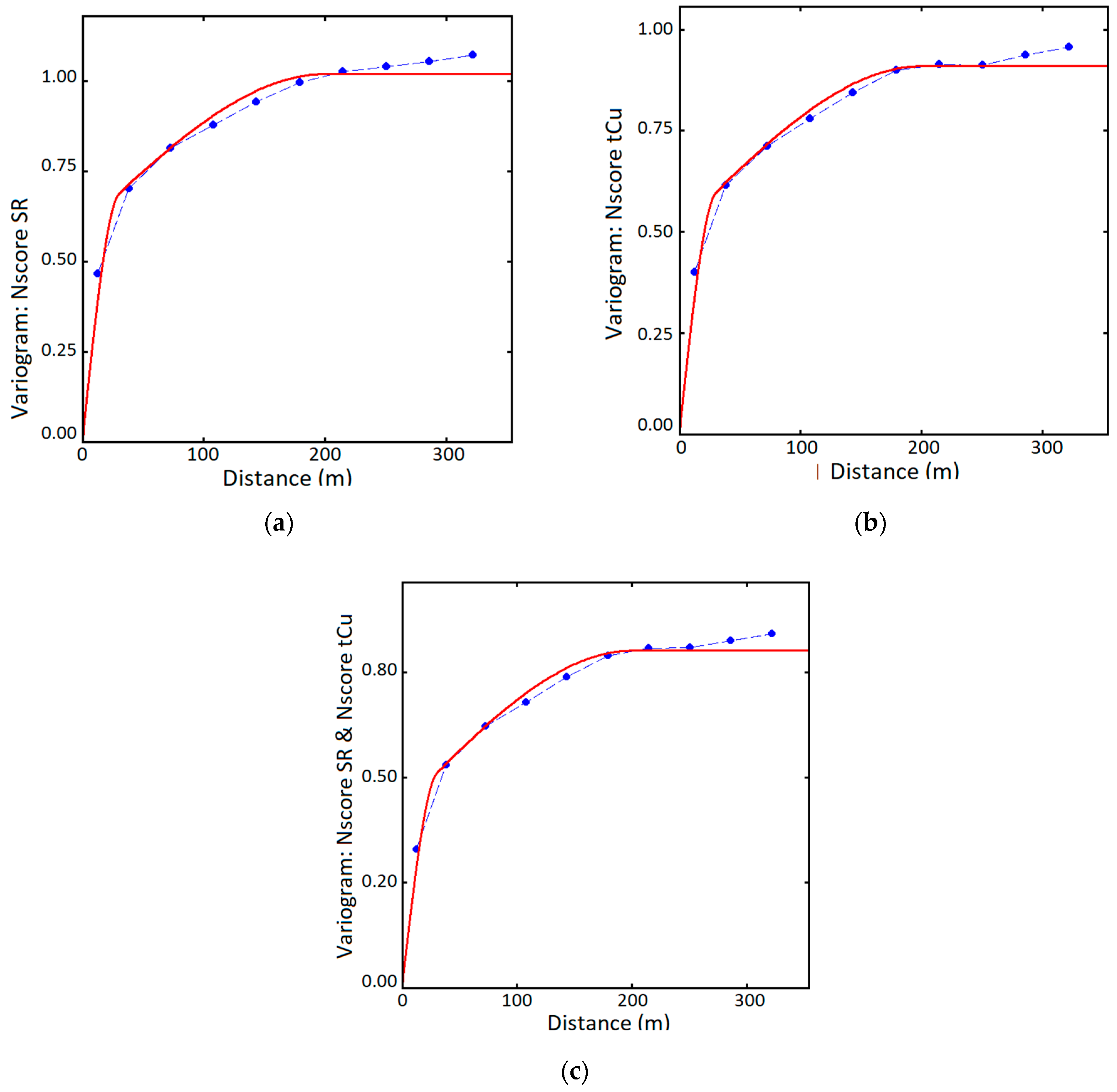
Direct and cross-variograms of normal score values of total copper grade and solubility ratio. (a) Direct variogram of SR (b) Direct variogram of tCu (c) Cross-variogram between SR and tCu.
Figure 7.
Direct and cross-variograms of normal score values of total copper grade and solubility ratio. (a) Direct variogram of SR (b) Direct variogram of tCu (c) Cross-variogram between SR and tCu.

Figure 8.
Cross-correlogram between MAF factors using the data-driven approach at different lags.

Figure 9.
Histogram of factors, showing normal score distribution.
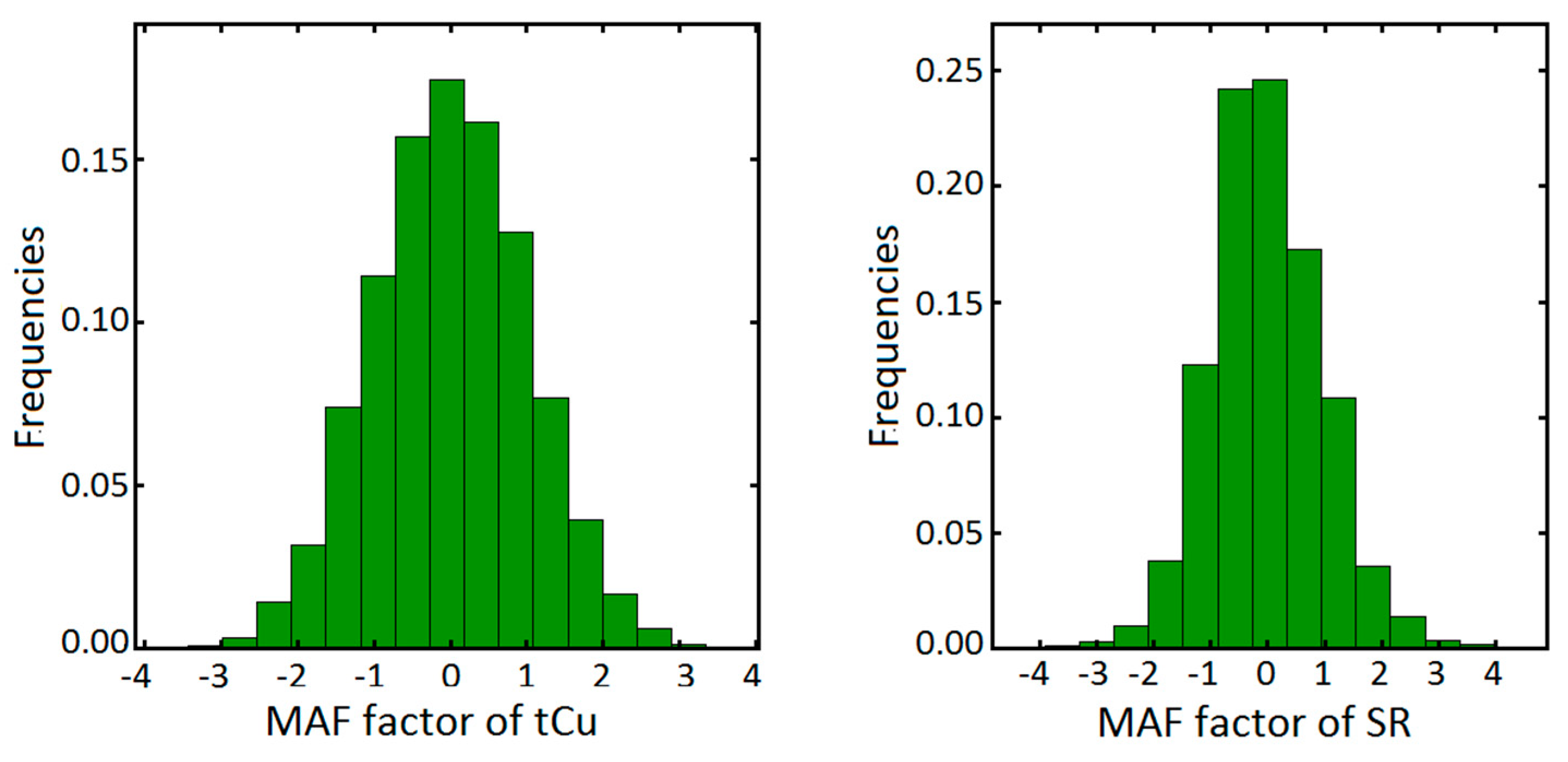
Figure 10.
Variogram analysis of each factor.
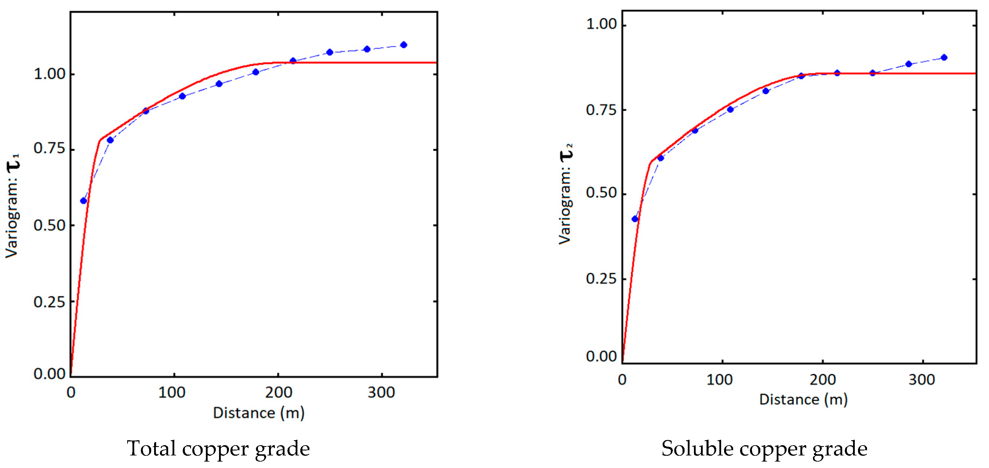
Figure 11.
E-type maps of simulated total and soluble copper grades by co-simulation approach.

Figure 12.
E-type maps of simulated total and soluble copper grades by MAF approach.
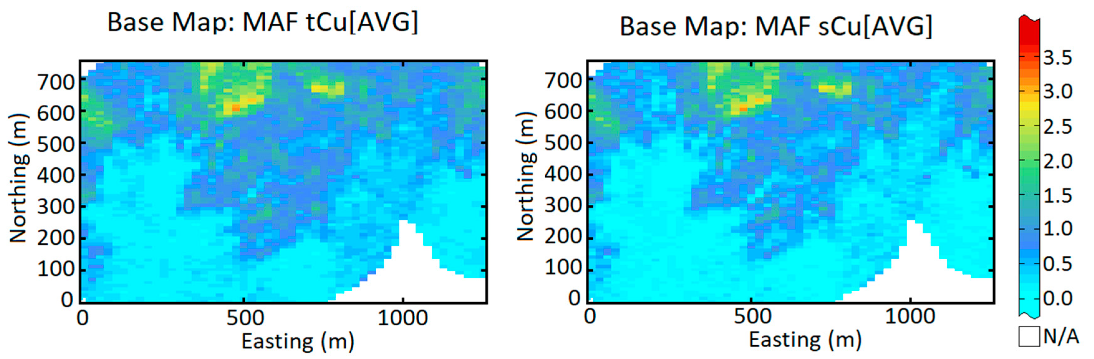
Figure 13.
The scatter plot of tCu(%) and sCu(%) obtained by MAF (left-up); TBCOSIM (right-up); original dataset (center-down) for realization No. 1.
Figure 13.
The scatter plot of tCu(%) and sCu(%) obtained by MAF (left-up); TBCOSIM (right-up); original dataset (center-down) for realization No. 1.

Figure 14.
Direct and cross-variograms of simulated realizations with TBCOSIM and MAF. (solid blue line: fitted model, dashed red line: average of the realizations; dashed green line: individual realizations). (a) Direct variogram of tCu(%) for TBcosim values; (b) Direct variogram of tCu(%) for MAF-TBsim; (c) Direct variogram of sCu(%) for TBCOSIM; (d) Direct variogram of sCu(%) for MAF-TBSIM; (e) Cross-variogram of tCu(%) vs sCu(%) for TBCOSIM; (f) Cross-variogram of tCu(%) and sCu(%) for MAF-TBSIM.
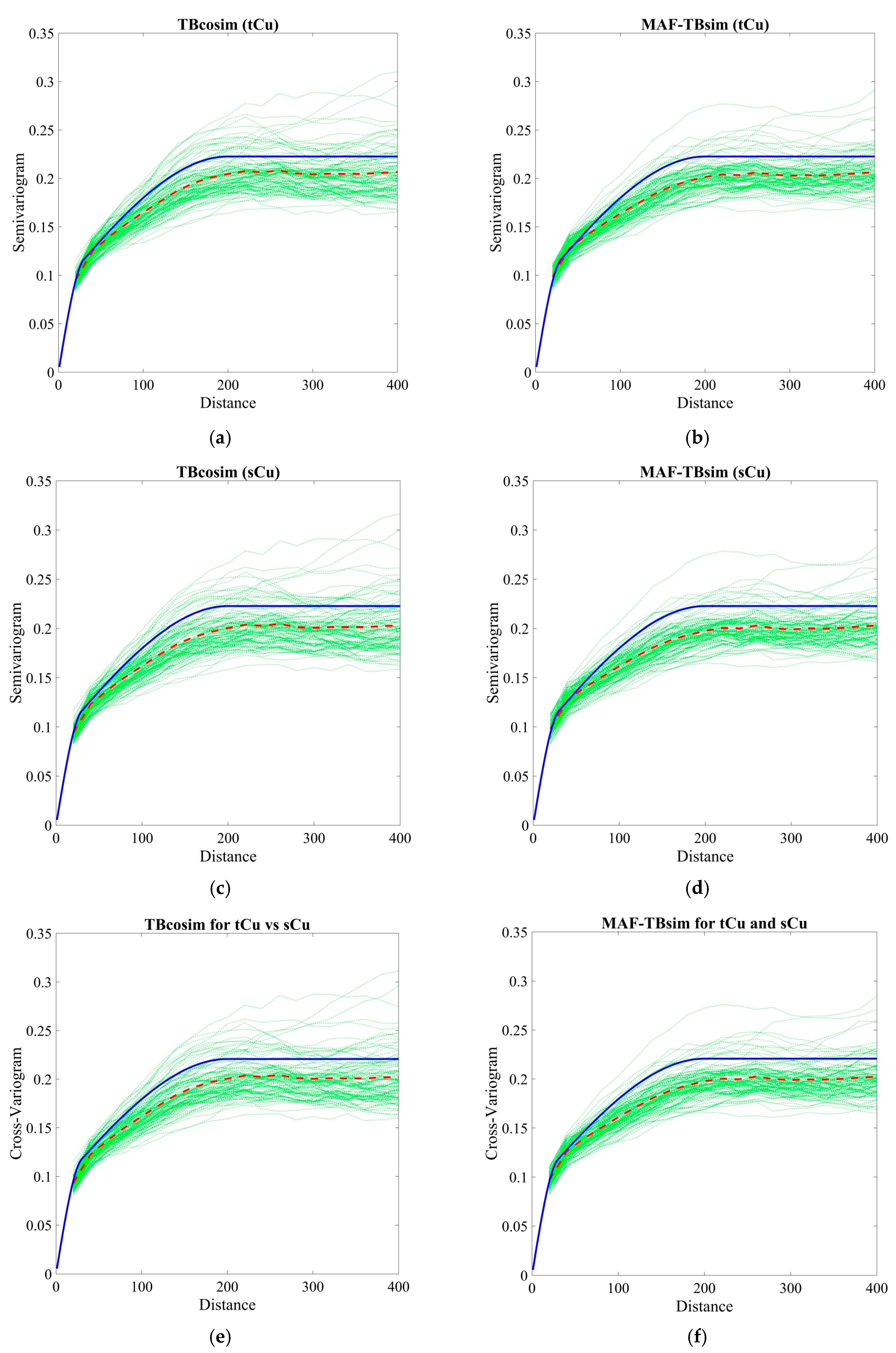
Figure 15.
Codispersion functions showing the same trend for both approaches (TBCOSIM and MAF) compared to original data.
Figure 15.
Codispersion functions showing the same trend for both approaches (TBCOSIM and MAF) compared to original data.
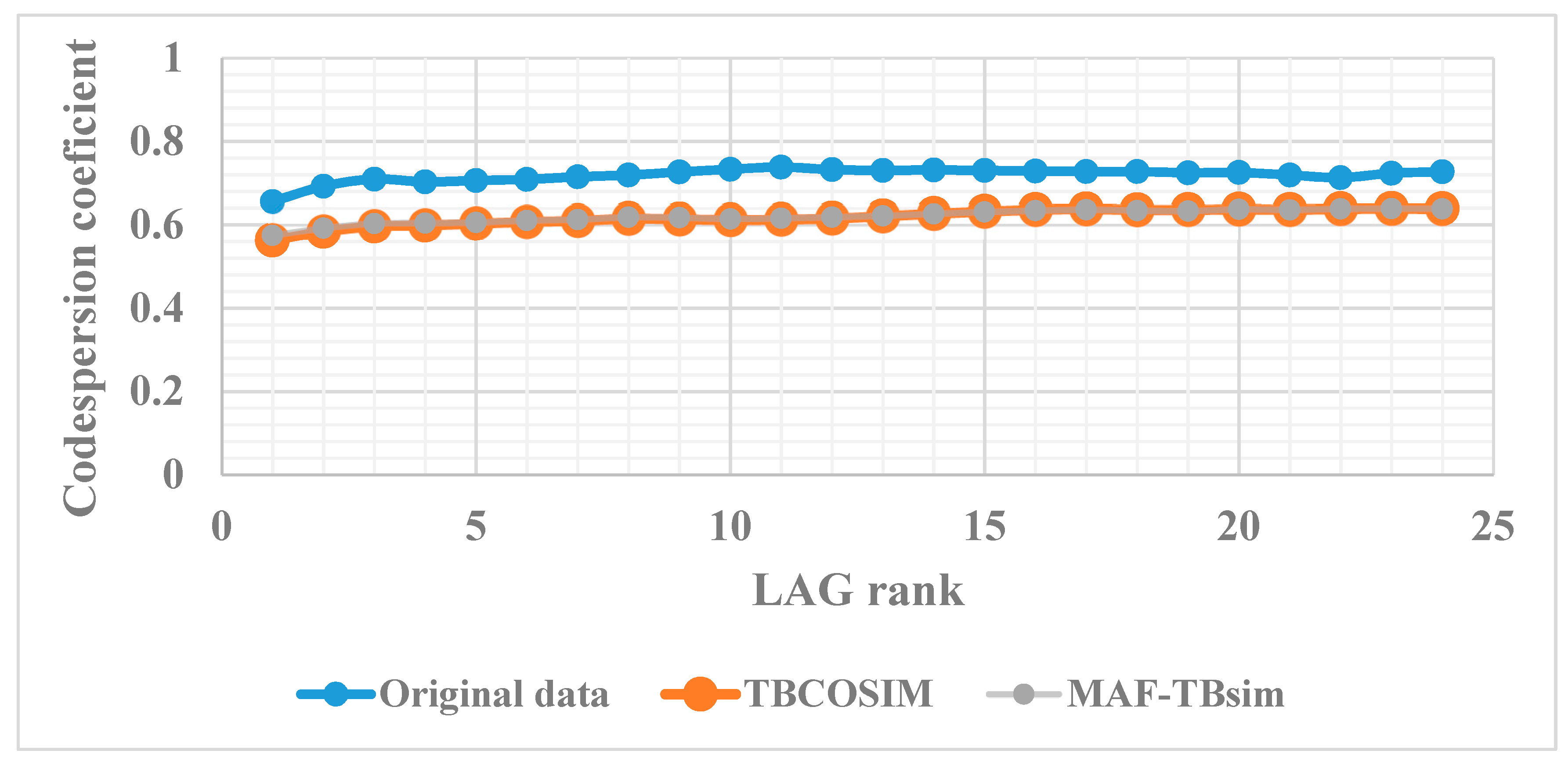
Figure 16.
QQ-plot of distributions of mean values of total and soluble copper grades for three different numbers of realizations (20, 50 and 100) obtained from TBCOSIM and MAF simulation. (a) Total copper grade; (b) Soluble copper grade.
Figure 16.
QQ-plot of distributions of mean values of total and soluble copper grades for three different numbers of realizations (20, 50 and 100) obtained from TBCOSIM and MAF simulation. (a) Total copper grade; (b) Soluble copper grade.

Figure 17.
QQ-plot of distributions of variances of total and soluble copper grades for three different numbers of realizations (20, 50 and 100) obtained from TBCOSIM and MAF simulation. (a) Total copper grade; (b) Soluble copper grade.
Figure 17.
QQ-plot of distributions of variances of total and soluble copper grades for three different numbers of realizations (20, 50 and 100) obtained from TBCOSIM and MAF simulation. (a) Total copper grade; (b) Soluble copper grade.

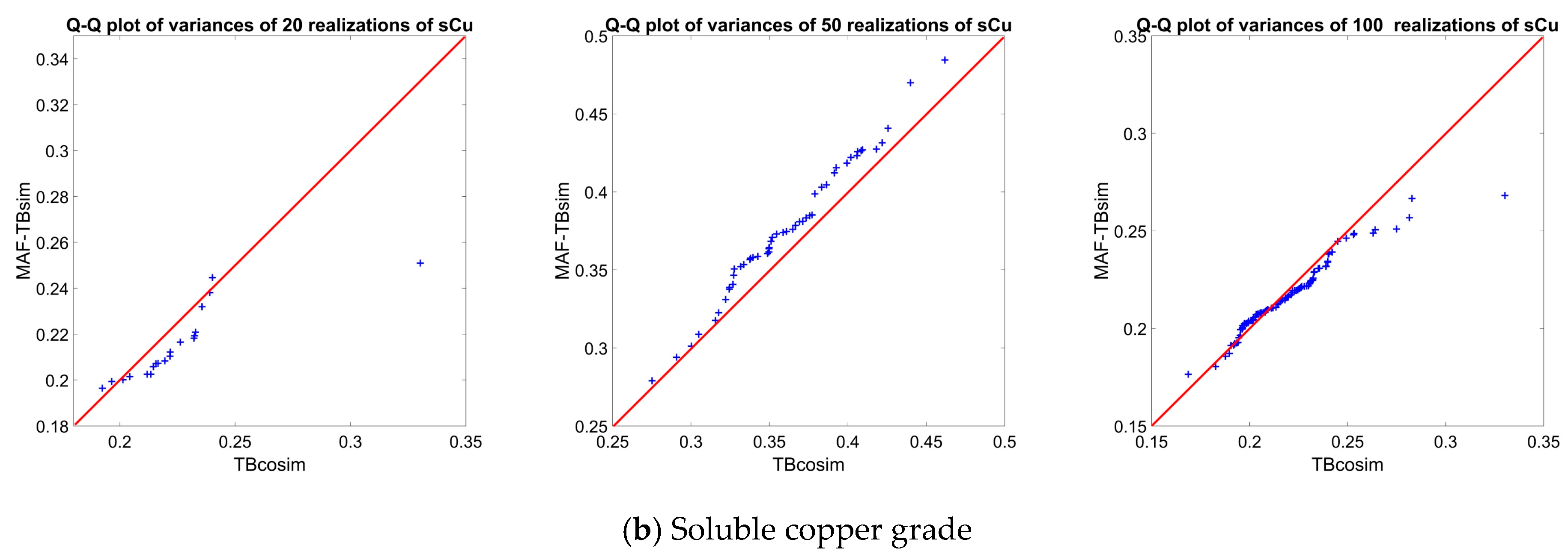
Figure 18.
Sensitivity analysis of mean values versus the number of realizations; blue line: MAF, black line: TBCOSIM and red line: original declustered line.
Figure 18.
Sensitivity analysis of mean values versus the number of realizations; blue line: MAF, black line: TBCOSIM and red line: original declustered line.

Figure 19.
Probabilistic domaining of geometallurgical domains in the oxide copper mine obtained from post processing of 100 realizations produced by MAF approach.
Figure 19.
Probabilistic domaining of geometallurgical domains in the oxide copper mine obtained from post processing of 100 realizations produced by MAF approach.
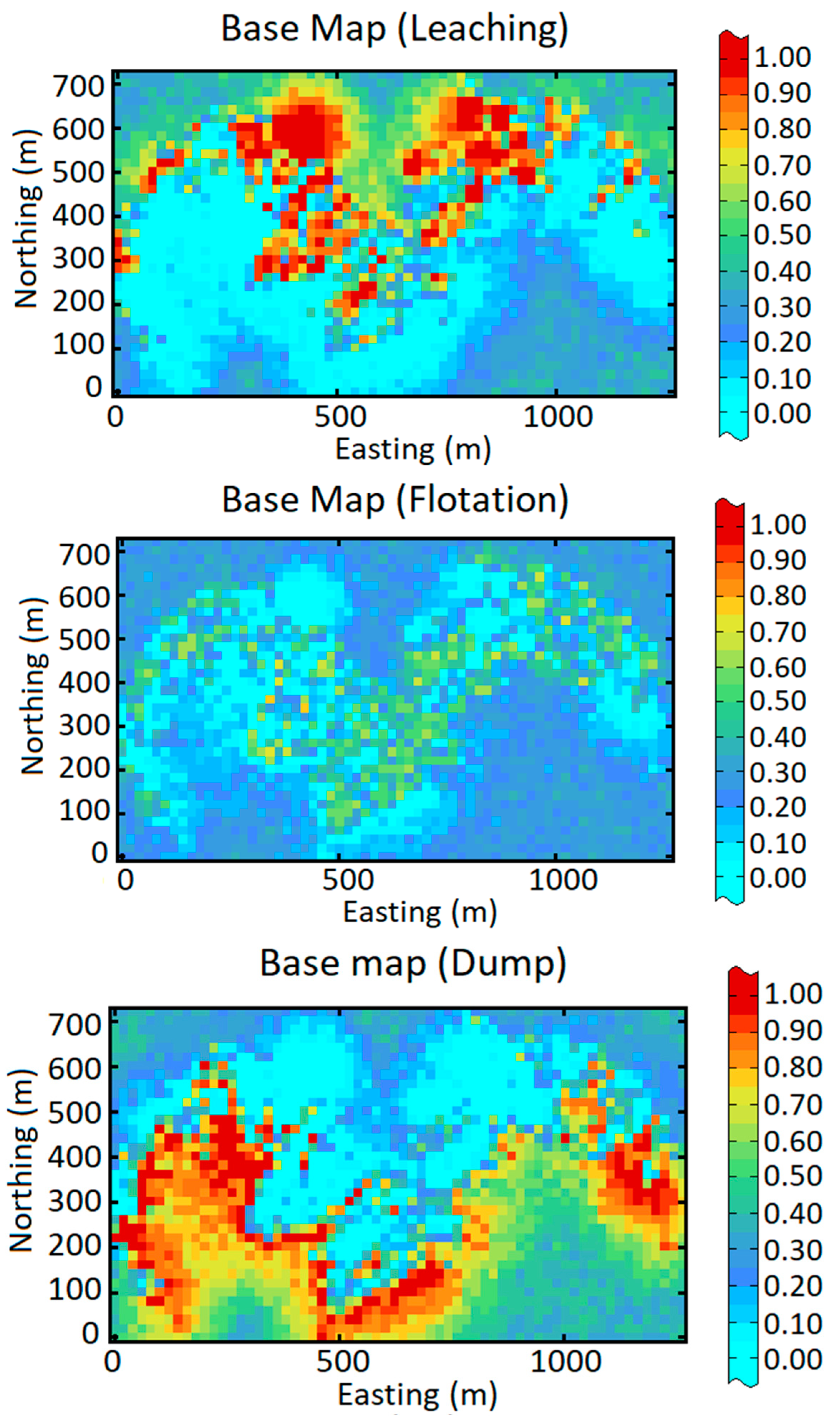
Figure 20.
Division of sample points into test and analysis for jackknife analysis; red points: analysis and black points: test.
Figure 20.
Division of sample points into test and analysis for jackknife analysis; red points: analysis and black points: test.

Figure 21.
Scatter plot for jackknife validation (prediction versus true values); left: MAF and right: turning bands co-simulation; black line: diagonal and red line: linear regression line.
Figure 21.
Scatter plot for jackknife validation (prediction versus true values); left: MAF and right: turning bands co-simulation; black line: diagonal and red line: linear regression line.

Table 1.
Statistical properties of tCU and sCu obtained from an oxide copper deposit mine.
| Variable | Mean | Variance | Maximum | Minimum | COV | |
|---|---|---|---|---|---|---|
| Original | tCu(%) | 0.723 | 0.233 | 3.150 | 0.100 | 0.667 |
| sCu(%) | 0.587 | 0.232 | 2.950 | 0.000 | 0.820 | |
| Declustered | tCu(%) | 0.632 | 0.209 | 3.150 | 0.100 | 0.723 |
| sCu(%) | 0.493 | 0.203 | 2.950 | 0.000 | 0.913 |
Table 2.
Reproduction of global mean, variances and correlations obtained from initial data, TBCOSIM and MAF over 100 realizations.
Table 2.
Reproduction of global mean, variances and correlations obtained from initial data, TBCOSIM and MAF over 100 realizations.
| Mean | Variance | Correlation | |||
|---|---|---|---|---|---|
| Parameters | tCu(%) | sCu(%) | tCu(%) | sCu(%) | tCu(%) vs sCu(%) |
| Original | 0.723 | 0.587 | 0.233 | 0.232 | 0.991 |
| Declustred | 0.632 | 0.493 | 0.209 | 0.203 | 0.989 |
| Average TBcosim | 0.616 | 0.487 | 0.228 | 0.219 | 0.990 |
| Average MAF | 0.611 | 0.483 | 0.225 | 0.216 | 0.990 |
Table 3.
Mean relative error obtained from TBCOSIM and MAF.
| tCu | sCu | |
|---|---|---|
| TBCOSIM | 0.284 | 0.678 |
| MAF | 0.268 | 0.667 |
© 2019 by the authors. Licensee MDPI, Basel, Switzerland. This article is an open access article distributed under the terms and conditions of the Creative Commons Attribution (CC BY) license (http://creativecommons.org/licenses/by/4.0/).
Share and Cite
MDPI and ACS Style
Abildin, Y.; Madani, N.; Topal, E. A Hybrid Approach for Joint Simulation of Geometallurgical Variables with Inequality Constraint. Minerals 2019, 9, 24. https://doi.org/10.3390/min9010024
AMA Style
Abildin Y, Madani N, Topal E. A Hybrid Approach for Joint Simulation of Geometallurgical Variables with Inequality Constraint. Minerals. 2019; 9(1):24. https://doi.org/10.3390/min9010024
Chicago/Turabian StyleAbildin, Yerniyaz, Nasser Madani, and Erkan Topal. 2019. "A Hybrid Approach for Joint Simulation of Geometallurgical Variables with Inequality Constraint" Minerals 9, no. 1: 24. https://doi.org/10.3390/min9010024
Note that from the first issue of 2016, this journal uses article numbers instead of page numbers. See further details here.