Forecasting Geoenvironmental Risks: Integrated Applications of Mineralogical and Chemical Data


1
ARC Transforming the Mining Value Chain Industrial Transforming Research Hub, University of Tasmania, Private Bag 79, Hobart, Tasmania 7001, Australia
2
CRC for Optimising Resource Extraction, University of Tasmania, Private Bag 79, Hobart, Tasmania 7001, Australia
*
Author to whom correspondence should be addressed.
Minerals 2018, 8(12), 541; https://doi.org/10.3390/min8120541
Submission received: 31 August 2018
/
Revised: 15 November 2018
/
Accepted: 19 November 2018
/
Published: 22 November 2018
(This article belongs to the Special Issue Geometallurgy)
Abstract
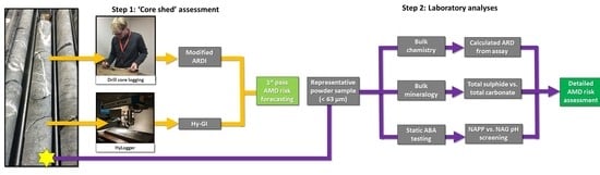
:Management of solid mine wastes requires detailed material characterisation at the start of a project to minimize opportunities for the generation of acid and metalliferous drainage (AMD). Mine planning must focus on obtaining a thorough understanding of the environmental properties of the future waste rock materials. Using drill core obtained from a porphyry Cu project in Northern Europe, this study demonstrates the integrated application of mineralogical and geochemical data to enable the construction of enviro-geometallurgical models. Geoenvironmental core logging, static chemical testing, bulk- and hyperspectral mineralogical techniques, and calculated mineralogy from assay techniques were used to critically evaluate the potential for AMD formation. These techniques provide value-adding opportunities to existing datasets and provide robust cross-validation methods for each technique. A new geoenvironmental logging code and a new geoenvironmental index using hyperspectral mineralogical data (Hy-GI) were developed and embedded into the geochemistry-mineralogy-texture-geometallurgy (GMTG) approach for waste characterisation. This approach is recommended for new mining projects (i.e., early life-of-mine stages) to ensure accurate geoenvironmental forecasting, therefore facilitating the development of an effective waste management plan that minimizes geoenvironmental risks posed by the mined materials.
1. Introduction
Porphyry systems are defined as large volumes (10 to 100 km3) of hydrothermally altered rock typically centered on porphyry stocks that may also contain skarn, carbonate-replacement, sediment hosted and high and intermediate sulphidation epithermal base and precious metal mineralization [1]. They are considered the hallmark of magmatic arcs, constructed above active subduction zones at convergent plate margins [2,3], though a minority occupy post-collisional and other tectonic settings that develop after subduction ceases [1]. Porphyry deposits are globally significant resources of Cu, Mo, and Au and supply 75%, 50%, and 20%, respectively, of the total production of these metals [1,4]. Typical hypogene porphyry systems have average grades of 0.5–1.5% Cu, <0.01 to 0.04% Mo, and up to 1.5 g/t Au with more variable Au and Cu grades associated with other mineralization compositions (e.g., skarns) [1,5]. The median global Cu composition for porphyry mines is around 0.5% and as such they are commonly regarded as “low-grade, large-tonnage” [6], e.g., Aitik mine, Sweden (1227 Mt reserves at 0.23% Cu) and Bingham Canyon, US (cumulative production of 2829 Mt at 0.7% Cu) [7]. Whilst porphyry deposits rank as 6th (calk-alkaline deposits) and 7th (alkalic) of 14 in terms of deposit types with acid and metalliferous drainage (AMD) potential [8], extraction of porphyry ores typically produces billions of tonnes of mine waste [9]. Sulphide minerals (e.g., pyrite, FeS2; and chalcopyrite, CuFeS2) are commonly observed in these wastes [10] and if surficially dumped, can undergo oxidation leading to AMD formation [11,12]. Techniques commonly used to predict AMD forming capacity rely on using total-sulphur values and a suite of laboratory-based static tests [11,12]. Whilst they provide quantitative information on how much acid or neutralizing capacity is offered per tonne of waste, testing a statistically significant number of samples can be financially prohibitive [13]. New tools are required by the mining industry to enable a large number of samples to be geoenvironmentally screened to facilitate better sample selection for static testing, as several limitations are still faced. First, pre-screening or proxy tests need to be introduced that focus on determining the geoenvironmental properties of drill core and will provide an insight into the overriding characteristics of the future waste (i.e., which sulphides dominate, abundance of carbonate neutralising phases). Second, the industry-wide perception that geoenvironmental classifications should be made after chemical testing of a pulverized sample in a laboratory needs to be challenged. Waste rock is fundamentally a mass of intact material, therefore, understanding the influence of texture and mineralogy is vital to determine: (i) how it will weather; and (ii) which transient minerals will form as surficial oxidation products. Third, utilizing data collected by other mine-site disciplines can cost-effectively assist in geoenvironmental pre-screening. For example, hyperspectral data using short-wave infrared data can be used to characterise drill core and waste materials [14,15,16,17,18,19], assay data can be used to calculate AMD [20,21] and automated mineralogical data can be used for waste characterisation following the methods described in [22,23,24,25]. By adopting a geometallurgical approach to this challenge, whereby proxy tests and methods to extract further information from existing datasets are developed and used as inputs for deposit-scale models, the opportunity is presented to adopt enhanced characterization practices.
Drill core collected in this study is from a porphyry Cu–Au–Ag–Mo prospect in Northern Europe.
Seven lithological units (volcaniclastite, clastic sediment, aphanitic porphyry, basalt, feldspar porphyry I and II, and dykes), subjected to hydrothermal alteration, dominate the deposit geology, with the porphyry units being notably more sulphidic. At this site, mining will likely proceed as an open-cut, thus, identifying and effectively using geoenvironmental characterisation tools that will enable deposit-wide domaining is a critical first step for mine planning. This paper introduces two new methods to facilitate this, a new geoenvironmental logging code and a new index by which to interpret hyperspectral data and shows how they can be integrated with routinely collected geoenvironmental data to efficiently forecast waste properties to support deposit-wide modelling.
2. Materials and Methods
2.1. Drill Hole and Pulp Sampling
Seven drill holes were examined in this study from both waste and ore zones. The waste holes (termed the W series) were taken to represent overburden which would have to be removed to provide access to the ore body as part of an open-cut project. Samples representative of the ore zone were primarily used to assist to evaluate calculated acid rock drainage (ARD) from assay approaches. One hole from the ore zone was also studied (OZ-1) to give an indication of the geoenvironmental behavior of the ore, in ARD terms, whilst stockpiled. The uppermost portion of these holes which intersected soil (e.g., to a depth of up to 7.1 m in W1) were not sampled. The shallow portion of the drill holes (up to 350 m depth) were studied and for every 3–5 m interval (on average), the drill core was wetted, photographed, and geoenvironmentally logged. Select samples (Table 1) representative of key geoenvironmental features were shipped to the University of Tasmania (UTas). Criteria for sample selection included: (1) Presence of several sulphide minerals (and in close/touching contact); (2) Presence of carbonates; (3) Co-occurrence of sulphides and carbonates; (4) Observation of sulphide weathering; and (5) Sulphides from different hydrothermal alteration zones. Sub-sampling of the available pulps (<63 µm, recalled from a commercial laboratory) was also undertaken with the objective of collecting pulps corresponding to geoenvironmentally logged intervals, and were also shipped to UTas. The general analytical protocol followed in this study was the Geochemistry-Mineralogy-Texture-Geometallurgy (GMTG) approach proposed by [26].
2.2. Geoenvironmental Logging
The most limiting factor when predicting AMD, during early life-of-mine stages, is the absence of mandatory and standardized textural analysis despite the control this has on weathering and acid formation when materials are dumped at surface. To address this, the acid rock drainage index (or ARDI) was proposed [27] so textural evaluations could be performed on drill core or waste rock particles. The ARDI assesses acid-generating sulphide minerals individually (recommended number of grains/particles for assessment = 20) on both the meso- and micro-scale in a given sample. Sulphides are assessed by five categories A to E which were specifically chosen based on their influence on acid generation. Parameters A, B, and C (ranked from 1–10) examine sulphide abundance, degree of alteration, and sulphide morphology, while parameters D and E (ranked from −5–10) assess the neutralising mineral content and the spatial relationship between acid generating and neutralising minerals as shown in Equations (1) and (2). Values derived from the meso- and micro-scale are averaged to give a final ARDI score (Equation 3).
where Me = Mesoscale phase; Mi = Microscale phase; A = content of acid generating phase; B = alteration of acid generating phase; C = morphology of acid generating phase; D = Content of neutralising phase; E = spatial relationship between acid generating and neutralising phase; X or Y = total score (/50); = total score for all phases; X1 = total for Me sample; Y1 = total for Mi sample.
Me = [A1–10 + B1–10 + C1–10 + D1–10 + E1–10] = X
Mi = [A1–10 + B1–10 + C1–10 + D1–10 + E1–10] = Y
High scores indicate acid formation, low scores indicate low-inert acid forming potential and negative scores indicate acid neutralising capacity (ANC). Scores from each category are totaled with values 50 to 41 considered as extremely acid forming (EAF); 40 to 31 as acid forming (AF); 30 to 21 are potentially acid forming (PAF); 20 to 0 are not acid forming (NAF); and −1 to −10 are classified as having ANC (Supplementary Table S1). ARDI values are screened against sulphur assay and paste pH data to allow for first-pass geoenvironmental domaining [26].
Whist the ARDI proposed by [27] required assessments to be performed on both a meso-scale and micro-scale, a modified ARDI was developed as part of this study to allow for the performance of simpler, more time-efficient assessments. An interval assessment [28] is first performed over a 1 m interval by assigning the modal proportion of sulphides (totaling 1) over the area. For example, if the sulphide mineralogy consisted of pyrite, arsenopyrite, and chalcopyrite in respective proportions of 30%, 20%, and 50% then scores of 0.3, 0.2, and 0.5 are recorded (Supplementary Figure S1). Next, an individual area equivalent to a standard field grain size chart (i.e., 8.5 cm × 5.5 cm) is targeted for ARDI assessment (Supplementary Figure S2). Where drill core is homogenous a representative area can be selected with ease. However, in other cases the area most dominated by sulphides was chosen for assessment as, for domaining, the most conservative ARDI value was sought. ARDI parameter assessments (A–E) are performed on each identified sulphide mineral type (Equations (4)–(6)) according to criteria specified in [17]. Total ARDI scores for each sulphide are then multiplied by their corresponding whole-interval estimations and values for each sulphide are summed to give a final ARDI score (Equation (7)). This score is then compared against the scoring criteria described above and given in Supplementary Table S1 and the interval is assigned a geoenvironmental risk ranking.
Sulphide 1 ARDI score × Interval proportion value = Sulphide 1 scaled ARDI value
Sulphide 2 ARDI score × Interval proportion value = Sulphide 2 scaled ARDI value
Sulphide 3 ARDI score × Interval proportion value = Sulphide 3 scaled ARDI value
[Sulphide 1 scaled ARDI value] + [Sulphide 2 scaled ARDI value] + [Sulphide 3 scaled ARDI value] = Modified ARDI value
2.3. Mineralogical Evaluations
2.3.1. Hyperspectral Mineralogy
The Australia-developed HyLogging™ systems are automated platforms to rapidly and systematically collect infrared spectroscopic reflectance data at dense sample spacing from drill core, chips, or powders. Mineral spectroscopy involves the capture of reflected, scattered, or emitted light from a sample with the variable light intensities recorded across hundreds of narrow contiguous wavelength channels by a spectrometer’s detector [19]. Each measurement generates a spectral response curve (spectrum) displaying relative absorption and reflection features (troughs and peaks) at specific diagnostic wavelengths [19]. This technique is responsive to the chemical composition and crystal structure of a mineral, therefore, mineral identification is possible based on the resulting “spectral fingerprint” or “signature” observed in the spectral response curve [13]. A select suite of minerals can be identified based on their diagnostic spectral absorption features displayed in the Visible to Near-Infrared (VNIR, 350–1000 nm), Short-Wave Infrared (SW-IR, 1000 to 2500 nm), and the Thermal Infrared (TIR, 5000 to 14,000 nm) region of the electromagnetic spectrum [13]. Continuous down-hole mineral information can be achieved, enabling modelling by providing information on the bulk rock and its inherent geological variability [19]. HyLogging has several advantages over other mineral identification techniques through its rapidity (up to 1000 m of core per day), its low cost per sample, and its non-destructive approach. Based on this, the potential application of HyLogger data is suited to geoenvironmental domaining at exploration/pre-feasibility stages of operations [18].
Each sampled drill core slab (n = 260) was scanned on the HyLogger HS3 system (Mineral Resources Tasmania, Tasmania, Australia). Prior to analysis, samples were cleaned with water and dried to remove dust. Approximately >5000 hyperspectral reflectance measurements were collected, with the data acquisition rate c.5 min for a three-section core tray. Measurements were captured from a 10 mm × 10 mm field-of-view along the middle of the core, and continuous linescan imagery across the full width of the core was synchronously acquired. Hyperspectral data analysis and mineral interpretation was performed in Version 8.1 of The Spectral Geologist (HotCore). The HyLogger attempts to identify three key minerals (min. 1, min. 2, and min. 3) present for each spectrum (of spectrally active minerals) collected. The TSG software reports the relative percentage abundance of up to three minerals (normalised to a sum of 1) for TIR and two minerals for visible near infrared- short wave infrared (also normalised to 1). Using these relative abundance values, a new TIR geoenvironmental forecasting index (termed the HyLogger Geoenvironmental Index or Hy-GI) is proposed. This calculation is adapted from the geoenvironmental domaining index (GDI) developed by [29] whereby for each identified mineral the neutralising potential (NP) value [30] and relative reactivity (or RR) value at pH 5 [31] are multiplied to give a geoenvironmental standard value (Equation (8); Supplementary Table S2). For each identified mineral, the geoenvironmental standard is multiplied by the relative intensity of the mineral reported by the HyLogger (Equation (9)). This calculation is repeated for each of the three identified minerals and the values are summed to give the final Hy-GI score (unitless) as summarised in Equation (10):
Neutralising Potential × Relative Reactivity = Geoenvironmental Standard
(HyLogger intensity × 100) × Geoenvironmental Standard = Min. value
Min. 1 value + Min. 2 value + Min. 3 value = Hy-GI score
The higher the score (i.e., 100,000: 100% calcite or 108,600: 100% dolomite), the greater the neutralising potential with both short-term (carbonates) and longer term (silicates) neutralisers appropriately considered [30]. The lower the score, the less neutralising with values < 1000 considered very weak neutralisers. If a value of 0 is assigned, then the sample is devoid of any neutralising minerals. In this study, Hylogging-derived mineralogy was compared against X-ray diffractometry (XRD) data to examine how accurate domaining neutralising capacity using carbonate relative intensity values and Hy-GI index values are.
2.3.2. Bulk Mineralogy
Sample pulps were analysed using XRD. A benchtop Bruker D2 Phaser X-ray diffractometer instrument with a Co anode X-ray source was used (UTas Laboratories, Tasmania, Australia). Prior to each instrument run, a corundum standard was analysed daily to check the X-ray beam alignment and ensure the correct collection of peaks. Each pulp sample (<63 µm) was hand-ground in an agate pestle and mortar (for up to 10 min) and loaded into an individual sample holder and loaded into the machine chamber. Experimental test work determined that a short sample run time (15 min) was suitably adequate to characterise the mineralogy of each sample and allow semi-quantificative Rietveld refinement. Each scan analysed between 5° and 90° (2θ) with a 0.02° step size and a measurement time of 0.4 s per step. A 1.0 mm (0.6°) fixed divergence slit, 2.5° soller slit, and a Fe-filter were used. Mineral phases were identified using Bruker DIFFRAC.EVA software (version 2.0, Bruker, Billerica, MA, USA) package with the PDF-2 (2012 release) powder diffraction file mineral database. Semi-quantitative modal mineralogy was determined by Rietveld refinement methods using Bruker’s proprietary software Topas version 4.2 (Bruker, Billerica, MA, USA)for typical limits of detection for this technique are between 0.5 wt. % and 1.0 wt. % modal abundance.
2.4. Bulk Chemistry
As whole rock assay data is collected routinely throughout at the early stage of a mining project, this data was used in this study to calculate ARD from assay following the methodology given in [14]. Pulp samples (n = 69) from drill holes W2 and OZ1 were selected as they represented typical waste/ore holes and were sent to ALS-Global for analysis (Method Codes: ME-XRF 26; ME-MS81; ME-MS42; S-IR-8; C-IR07; ME-ICP41 with 69 elements measured including Al, Si, Fe, Na, Mg, Ca, S, As, Cu, Cd, Pb, Zn). Sample duplicates were also analyzed with NATA accredited laboratory quality assurance/quality control protocols followed. To perform calculated mineralogy from assay two methods were used based on the presence/absence of corresponding XRD data. Where XRD data were present (and had been quantified using Rietveld refinement methods) a training set was developed using a weighted least squares method [20]. In this study, the abundance of 27 distinct mineral compositions were calculated. For data without corresponding XRD, linear programming using the Simplex method was followed with the previous training set used to calibrate the objective functions [20]. In this method, as in the weighted least square method, calculated mineral abundances were limited to ≥0 and ≤100%. The calculated mineralogy data were multiplied by acid producing/neutralising potential factors as described in [20].
2.5. Static Testing
Paste pH and net acid generation (NAG) pH testing were performed on pulp samples (<75 µm). Paste pH testing followed the ASTM D4972-01 (2007) methodology [32] whereby the sample is immersed in pH in a 0.01M CaCl2 solution at a 1:1 solid to solution ratio. The pH value of each sample (n = 206) was measured in triplicate, with the standard deviation for 99% of samples calculated as <0.1. Samples (n = 59) for net acid generation (NAG) testing were selected based on GMTG approach stage-one screening results (i.e., classifications assigned from a combined screening of ARDI, paste pH, and total sulphur values) for samples from waste holes only (W1, W2, W4, and W5). As all samples selected for NAG testing contained STotal greater than or equal to 0.3%, a modified multi-addition NAG procedure was used, whereby 30% H2O2 (hydrogen peroxide) was added (traditionally 15% H2O2 is used). This modification was proposed by [33] as scanning electron microscopy investigations on NAG test residue material showed partially reacted pyrite grains remained after oxidation with 15% H2O2. An aliquot of 50 mL of H2O2 was added to the samples and allowed to react for two hours. Following this, the samples were heated to ~60–65 °C using a laboratory hot plate for one hour. They were cooled, and the process repeated twice over, but with the quantity of H2O2 increased to 100 mL. The pH and electrical conductivity (EC) measurements were collected in triplicate. Maximum potential acidity (MPA) was calculated from sulphur assay data provided by the site. Sobek testing to calculate acid neutralising capacity (ANC) was only performed on samples that were NAG tested (ALS Global, Method Code EA 013) to enable the calculation of the net acid producing-potential or NAPP (MPA (Stotal × 30.6) − ANC) for screening against NAG pH values [12]. These results were compared against the geoenvironmental classifications derived from geoenvironmental logging, mineralogical, and assay data to determine if the combined use of these new methods can independently classify waste properties correctly.
3. Results
Whilst several acid and metalliferous drainage prediction methodologies were performed in this study, this section presents a snapshot of key results with a focus on (1) describing the lithological characteristics of the sampled drill core in AMD terms; and (2) critically evaluating data from new methodologies compared to traditionally derived AMD data with a focus on waste drill holes.
3.1. Geoenvironmental Logging Assessments
3.1.1. W-1
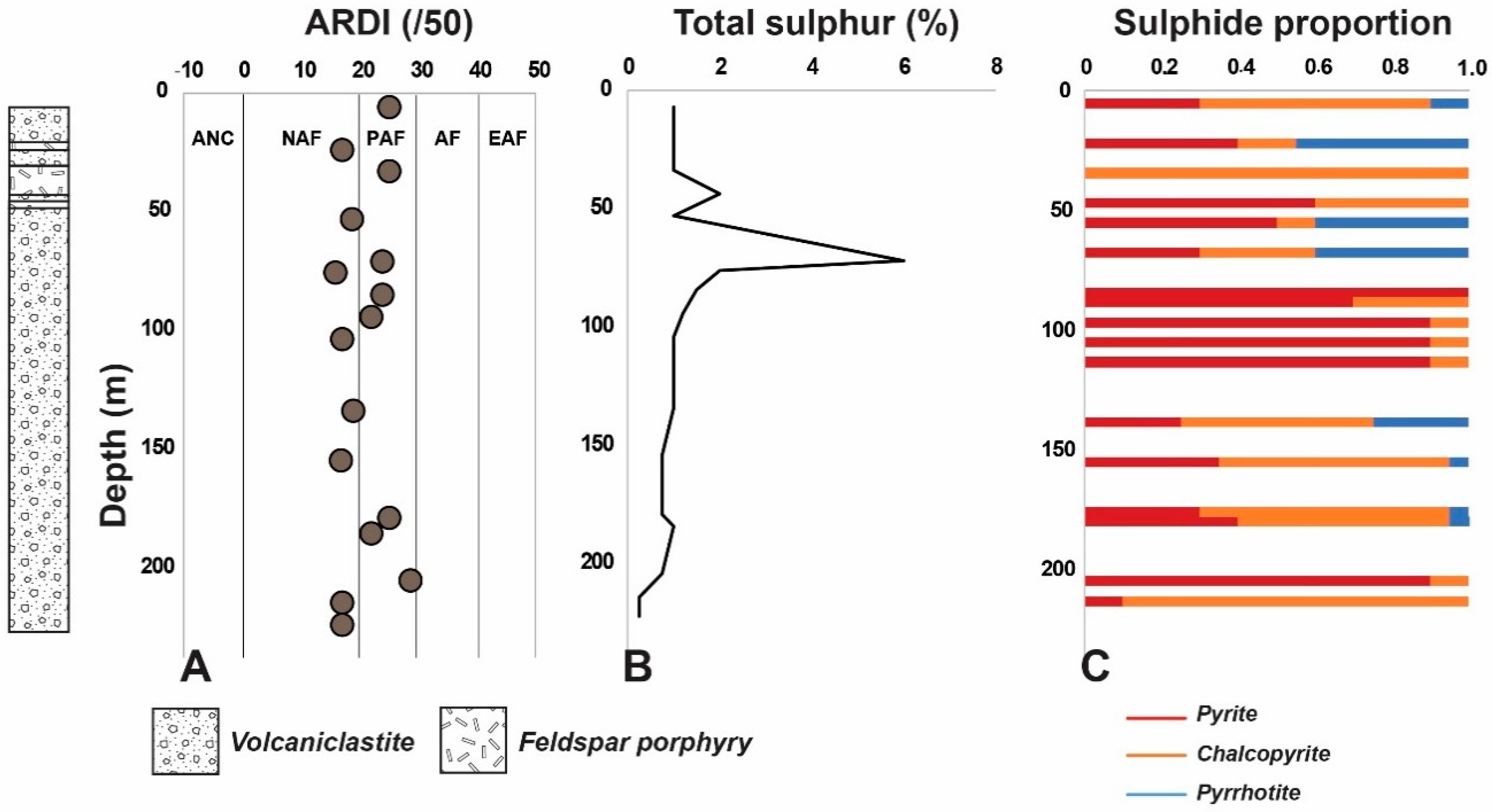
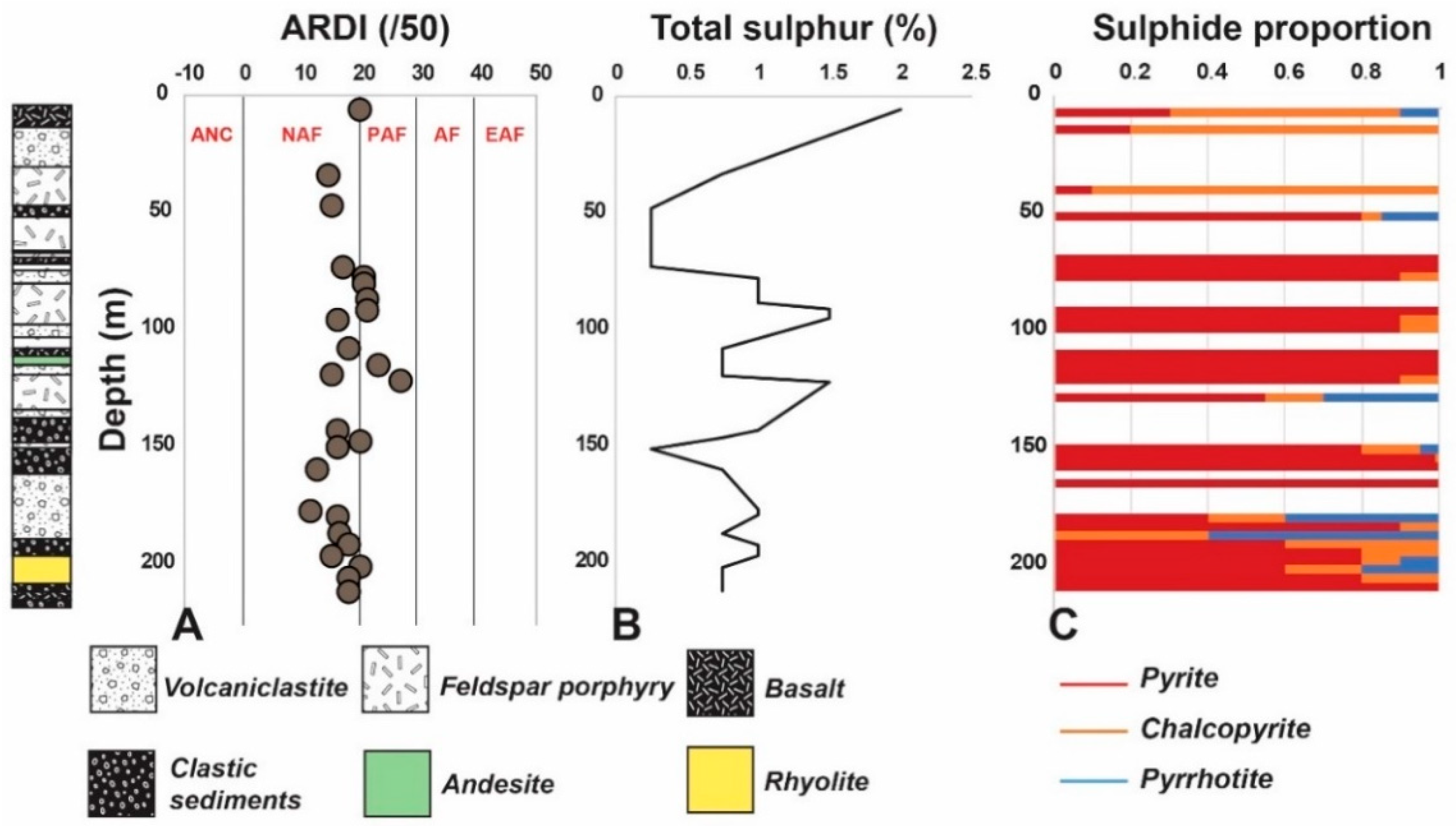
The dominant unit within this hole is the volcaniclastite—a matrix supported, polymict breccia containing sub-rounded clasts (Figure 1). Varying degrees of clast alteration was noted with local examples of unaltered feldspar-phyric equivalents observed. Overall, the presence of pervasive quartz alteration obscures breccia textures making it difficult to differentiate between clasts and matrix. Approximately 5 to 10 m thick intervals of feldspar porphyry form small fingers within the volcaniclastite in the top ~60 m of the hole, highlighting the intrusive nature of the unit. Feldspar phenocrysts dominate, giving the unit an overall porphyritic texture. Quartz eyes/phenocrysts are also common within this unit. Additionally, a breccia facies containing highly silicified-matrix supported sub-angular clasts was identified at the base of the drill hole (between 214.2 and 226.25 m depth) and classified as NAF by the ARDI with 0.25% total sulphides (pyrite = 0.9, chalcopyrite = 0.1, pyrrhotite = 0; Figure 1C). Alteration minerals include illite, kaolinite, chlorite, and sericite. Pyrite, pyrrhotite, and chalcopyrite were identified in both the volcaniclastite and feldspar porphyry. Visually, total sulphide abundance increased towards the centre of the studied portion of the drill hole (from 43.7 m to 104.2 m; Figure 1). From 104.2 m to 226.25 m sulphide abundance decreases, with the total abundance measured being <1%. Pyrrhotite is observed in the upper 50 m, decreasing between 50 and 100 m depth and increasing in abundance from 130 to 200 m (Figure 1C). Beyond 160 m depth, chalcopyrite, which is less acid forming than pyrite [12], is dominant (Figure 1).
3.1.2. W-2
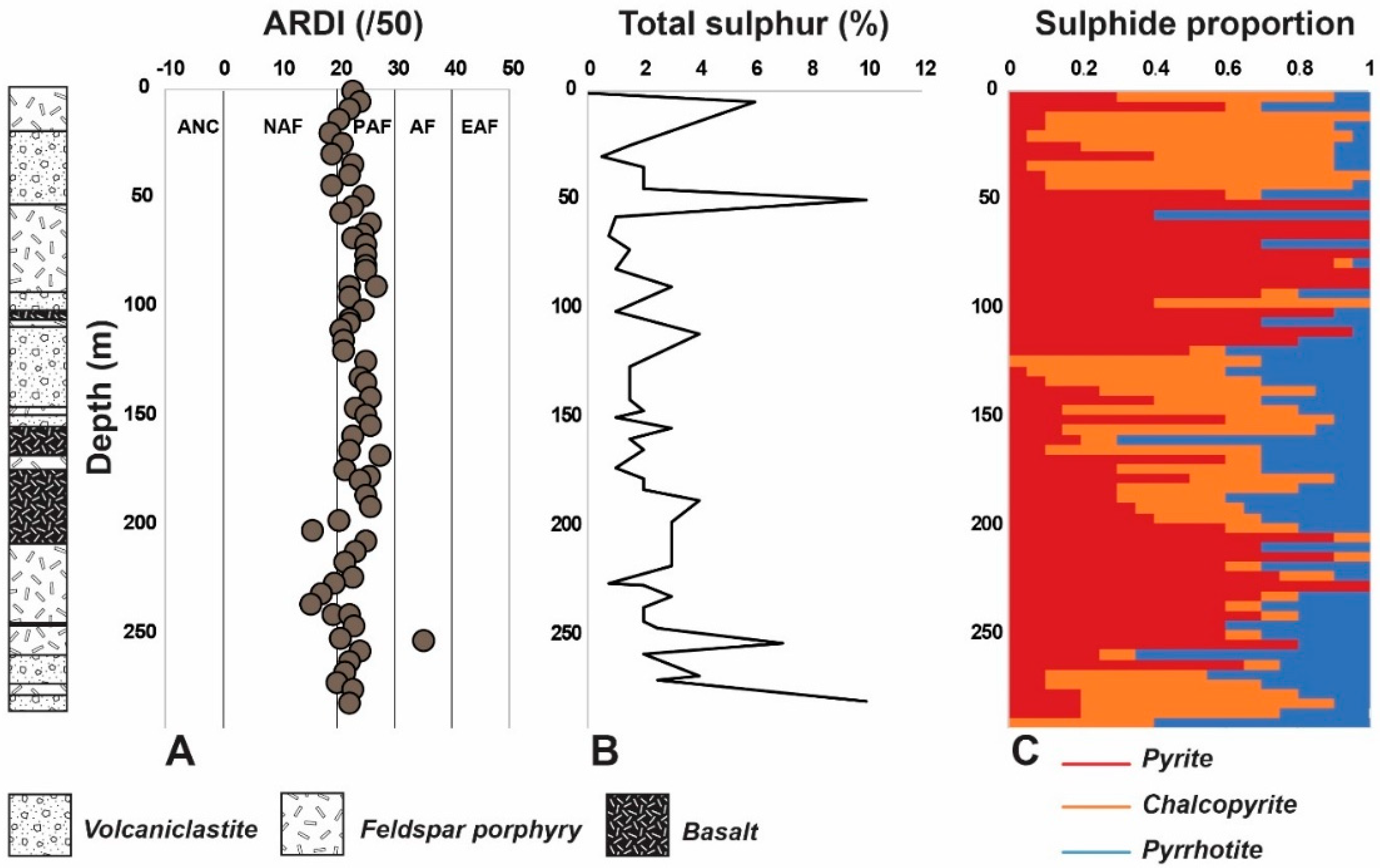
In this drill hole, basalt forms discrete intervals between 1 and 5 m thick within the dominant volcaniclastite and feldspar porphyry units (Figure 2). The exception to this is the presence of a 36 m basaltic interval from 172 to 208 m. The ARDI scores are within the PAF field with four plotting as NAF (feldspar porphyry and basalt units) and one as AF (feldspar porphyry). Total sulphur varies significantly down hole, ranging from 0.5% (30.1–35 m) to 10% (e.g., 50–52.8 m; Figure 2B). In general, the feldspar porphyry is dominated by pyrite (Figure 2C), particularly towards the centre and base of the observed section of this drill hole. Conversely, the volcaniclastite is typically chalcopyrite-rich, although exceptions to this do occur (e.g., 93–96.2 m). Pyrrhotite is also common in this rock type, however at ~0.3 total abundance (Figure 2C). Common silicates observed include quartz, chlorite, and sericite, suggesting these samples are from a chlorite–sericite alteration zone defined by [1]. It is noteworthy that mineralogical observations made during ARDI logging recognised the presence of magnetite, typically as veins, locally associated with carbonate. Further, isolated occurrences of molybdenite occur within quartz veins. Garnet was also noted in the top 15 m, alongside thick carbonate veins (~2 cm), which may reflect a potential skarn-style alteration zone.
3.1.3. W-3
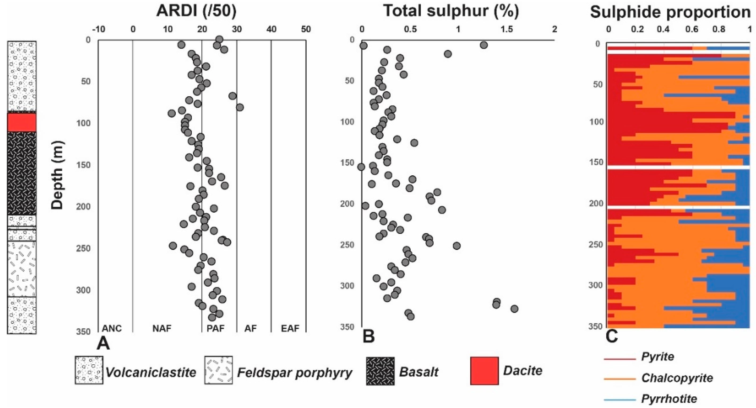
Geological units encountered in this hole were more variable than the previous two, with shallow dacite (30 m thickness) and a significant basalt unit (100 m thickness) observed with volcaniclastite and feldspar porphyry units enveloping them both.
ARDI values were variable with roughly a split between NAF and PAF fields (Figure 3A), with one sample again plotting in the AF field (ARDI score: 31/50; 84.8 to 88.2 m; dacite). Total sulphur values enabled the refinement of these classifications with five main zones of PAF material observed (Figure 3B), the majority of which fall into volcaniclastite zones (at approximately <10 m, 120 m, 160–210 m, 240 m, and 320–350 m). At shallow depth, pyrite and chalcopyrite dominate in the volcaniclastite units with pyrite dominating in the andesite unit (Figure 3C). In contrast, chalcopyrite dominated in the feldspar porphyry unit, and the deeper volcaniclastite unit, which appeared to have been chlorite-altered, contained much less pyrite than the shallower expression of this unit. Molybdenite (2–4 mm anhedral grains) was also observed at depth in this unit. Calcite was contained within the thick basalt unit and was present as veinlets (up to 5 mm width). Calcite was also observed in the feldspar porphyry unit (e.g., 242 m) however it was directly associated with pyrite in veins, and therefore ARDI values were in the PAF realm. Both units are altered to an assemblage of calcite, chlorite, and plagioclase with minor epidote consistent with propylitic alteration. At the base of the drill hole, potassium feldspar, biotite, and magnetite were observed, suggesting that this hole intersects a transition from propylitic to potassic alteration zones.
3.1.4. W-4
Volcaniclastite, feldspar porphyry, basalt, and a matrix supported (chlorite-altered) fault breccia containing extensively potassium feldspar-altered angular clasts (Figure 4) were identified in this drill hole (characteristic of the potassic alteration). Carbonate was observed as veinlets or replacement of host rock during ARDI logging, throughout the drill hole with basalt dykes, rhyolite, and andesite horizons also observed (Figure 4). Orthoclase alteration was found to be increasing towards the base of the studied portion of the drill hole. As this appears congruent with fault breccia clasts, it may be related to this faulting event. Additional logged alteration minerals include epidote and chlorite stringer veins and alteration patches with dendritic chlorite veinlets consistent with propylitic alteration. Based on sulphide and carbonate abundance, and sulphide textural expression, most samples were classified as NAF from ARDI logging with only 21% classified as PAF (Figure 4A).
Total sulphur values were high with approximately 50% of samples plotting above the 0.3% cut-off and the sulphur content generally increasing with depth (Figure 4B). Overall, the upper portion of this drill hole (i.e., above approximately 80 m) appears less acid forming (majority of samples NAF) and as depth increases, so does the acid-forming potential. Generally, disseminated pyrite was dominant, followed by disseminated-clotted chalcopyrite. Pyrrhotite was present in minor amount within some intervals (e.g., 48.05–53 m); however, it was typically absent. Between 13.65 and 18.35 m, no sulphides were observed, and thus a potential neutralising capacity or PNC/NAF classification was given.
3.1.5. W-5
The portion of the drill hole examined was dominated by the clastic sediments unit with interbedded volcaniclastite units at shallow depth and one basalt dyke intrusion (at approx. 248–249 m). ARDI values were dominantly NAF (i.e., below 20; Figure 5A) with some values falling into the <10 category suggesting the presence of carbonates in this lithology. Paste pH values show that the volcaniclastite unit is potentially more acid forming than the clastic sediment unit as the PAF values shown in Figure 5B correspond with this horizon. Two samples are highly sulphidic (Figure 5B) at 270.6–271.3 m and 304–304.65 m depth (clastic sediment). ARDI values do not amplify this as both are also carbonate-bearing which is considered in the ranking. Quartz and sericite dominate the silicate mineralogy suggesting these samples represent the phyllic alteration zone. Pyrrhotite is the dominant sulphide in contrast to the previous holes.
3.2. Carbonate Mineralogy
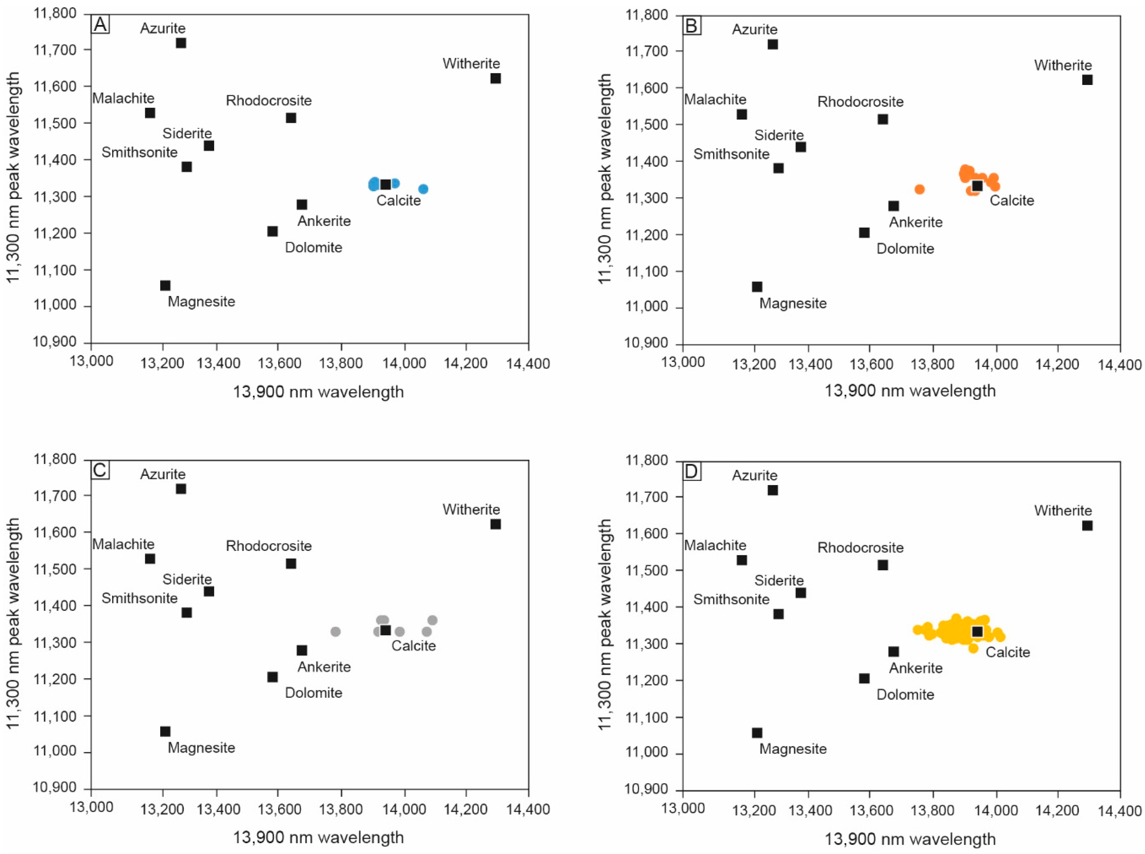
The pre-screening assessments identified presence of minor carbonate minerals (including as vein infill). Hyperspectral drill core scanning was performed to confirm their presence and better constrain the carbonate mineralogy given each carbonate mineral has different neutralising potential values. Carbonate minerals have diagnostic spectral peaks at around 6500 nm, 11,300 nm, and 13,900 nm (in the TIR region). Using the measured peak positions for the carbonates TIR data was plotted using the scalar developed in [19] as shown in Figure 6. For W1, plotting carbonates in this manner was not possible as no spectral features were reported for the 11,900 nm (or 6500 nm) features. For the other waste holes, where detected, the composition is dominantly calcitic (with a calculated absolute ANC of 1000 kg H2SO4/t). For most of drill holes, effective acid neutralising capacity existing as calcite [19] is present. However, a compositional trend towards Mn end-members is seen for W3 and W5 (Figure 6). Ankerite has a lower neutralising capacity than calcite (970 kg H2SO4/t), therefore, the effective ANC available is lower than would be perceived if the carbonate type had not been specified and instead was assumed as calcite. Thus, using TIR data can be a complimentary static testing tool to use as opposed to performing acid-buffering characteristic curve tests for which data interpretation can be difficult [11,12].
To further interrogate where units with neutralising potential reside (although ARDI values suggest these to be infrequent) the Hy-GI calculation was performed on this dataset. The Hy-GI scores are quite varied across these holes, but all plot below 800, with many reporting 0, confirming an overall deficiency in neutralising capacity in this deposit (Figure 7). Therefore, AMD formation from all units is probable when considering the abundance of sulphides in these materials as shown in the downhole sulphide abundance plots in Figure 1, Figure 2, Figure 3, Figure 4 and Figure 5. W1 (dominated by the volcaniclastite unit) has the least amount of neutralising capacity and could be considered to have negligible/inert capacity given that values for some samples are <100 (e.g., 96.7 m). In W2, the neutralising capacity notably increases with at least five samples (in the basalt unit) assigned higher scores, but these are discrete occurrences. W3 has the greatest neutralising capacity of all (correlating with the basalt unit) studied waste holes based on calculated Hy-GI values, (particularly from 111.6 m to 216.9 m). Towards the base of this hole where Hy-GI values increase, the volcaniclastite unit is logged, suggesting that the proportion of carbonate veins is also distributed at deeper parts of this unit. Similarly, high Hy-GI values are reported at that top of W4 which once again, correlates with the presence of the basalt unit. W5 has several discrete occurrences of potential neutralizing capacity, but unlike other drill holes, the neutralising potential is observed throughout the clastic sediment unit.
3.3. Calculated ARD from Assay
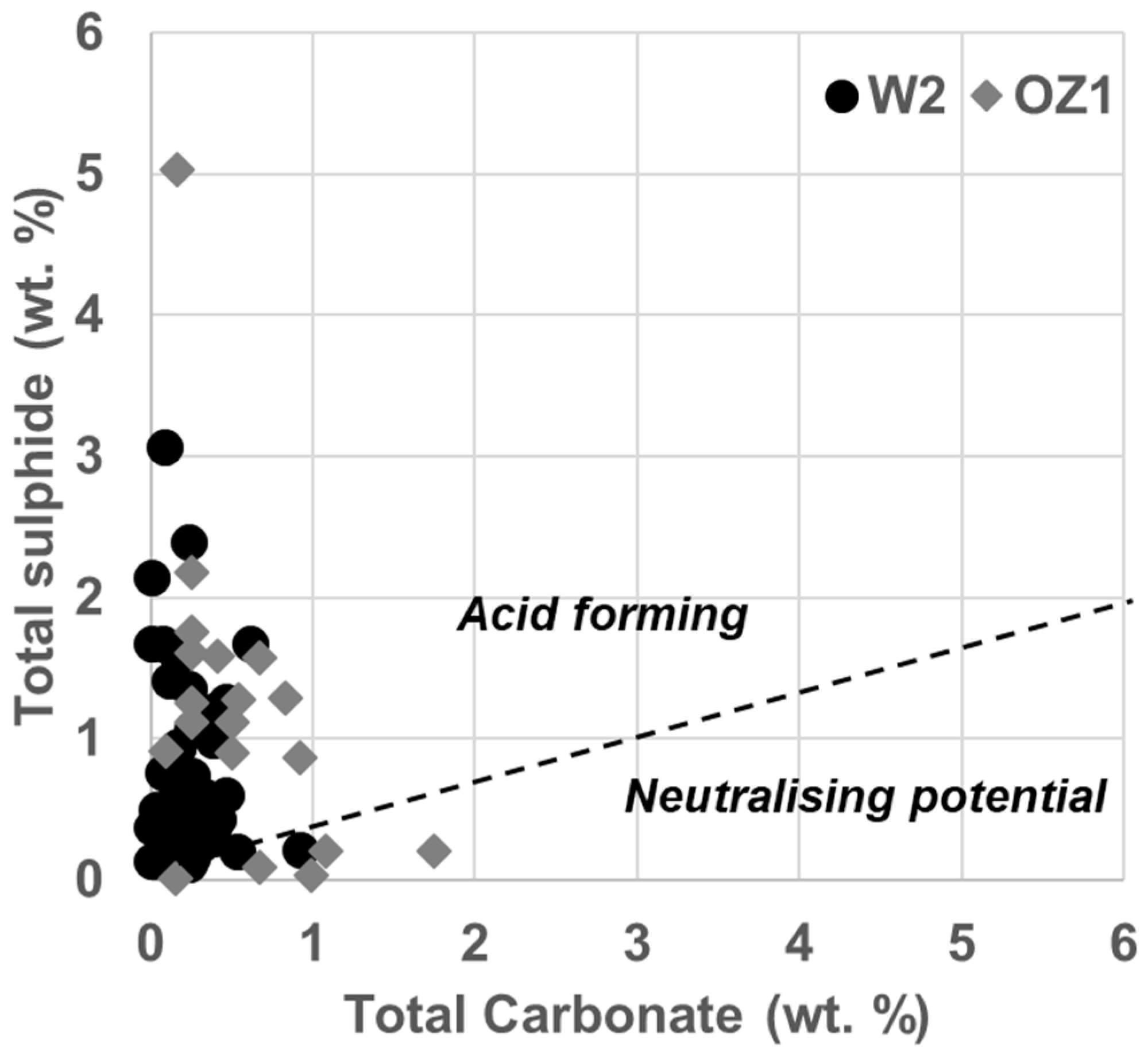
A growing trend of using assay data to calculate mineralogy has been noted [21] therefore calculating ARD generating potential is a beneficial way to use these data. To enable the calculation, 13 samples from W2 and OZ1 (dominated by altered diorite, tuff, andesite, and rhyolite units; Table 1 were used as the training set with their values (Supplementary Table S3) compared with those calculated from quantitative XRD. The correlation for carbonates was positive (>R2 = 0.88) suggesting that using these calculated values for neutralising potential domaining is acceptable as part of a geoenvironmental forecasting approach. The trained algorithm was applied to samples across the entire of the two drill holes W2 and OZ1 and a total sulphide vs. total carbonate ARD plot (following [34]) was constructed based on the resulting data (Figure 8). Only nine samples were recognised as having a net neutralising potential (with the majority of these from OZ1) though it is noted that neutralising potential based on these calculated mineralogy values (following [20]) are very low for these samples (i.e., <1 kg CaCO3/t). The overall acid forming capacity was calculated (also following the methodology given in [34] and described in [20] with a range of 0.1 to 82 kg H2SO4/t (average: 14 kg H2SO4/t). When screened against total sulphur values (Figure 9) these samples classify as PAF with samples from both drill holes falling into the PAF-high capacity quadrant (i.e., towards the upper right-hand corner of the plot). The calculated correlation fit between these data indicate that ARD assay calculations, for this dataset, are likely correct (R2 = 0.98).
3.4. ABA Classification
Comparison of NAPP against NAG pH values (as is convention in waste classification assessments—see [12]) confirms the characteristics predicted by these mineralogical techniques and illustrates that many samples are PAF with very little buffering capacity offered by any of the encountered waste lithologies (Figure 10). The highest risk samples were from W2 volcaniclastite, 50 m depth; Figure 10) and W5 (clastic sediment, 270 m depth; Figure 10). Several samples from W4 with 2 samples from the feldspar porphyry and basalt units plotting in the uncertain field (Figure 10). These carbonate-bearing samples containing low sulphur and correspondingly low negative NAPP values were calculated. Potentially, the NAG pH value should have been higher, but based on XRD classifications, the 3:1 total carbonate (i.e., summation of the modal abundance of carbonate minerals) to total sulphide (i.e., summation of the modal abundance of sulphide minerals) criterion, as proposed by [34], is not met to classify it as NAF thus these are most likely also PAF (Figure 11). Only three samples from W5 (clastic sediment) are classified as having neutralising capacity based on mineralogy (Figure 11). Overall, these classifications agreed with observations made when classifying using paste pH (not shown), ARDI and total sulphur values therefore confirming that very little effective ANC exists in the waste units encountered in this study and validating ARDI, Hy-GI and calculated ARD from assay classifications.
4. Discussion
4.1. Waste Mangement Planning
Forecasting the geoenvironmental properties of an ore deposit can assist with building a general understanding of its common characteristics enabling early identification of potential waste management issues and rehabilitation planning [35,36,37]. However, these characteristics can only be ascertained following the analyses of a large number of samples [38], and for several units encountered in this study, a statistically significant number were not collected (e.g., dacite, Table 2). The sampled waste holes studied have PAF characteristics as shown in Table 2 (note, mineralogy per lithotype is not shown as differential hydrothermal alteration styles have been experienced across drill holes and at different depths). From these samples, both the volcaniclastite and clastic sediment units present a potential geoenvironmental risk with the high ARDI and total sulphur; low ANC and NAG pH values (i.e., <pH 2.8). The only waste unit recognized as potentially offering net-acid neutralising capacity is the basalt unit (with the lowest NAPP value), but its distribution is sporadic. Many samples from the chlorite–sericite, phyillic, propylitic, and potassic alteration zones have been sampled in the waste holes as the drill core observations and measured mineralogical assemblages suggest. Phyllic alteration is recognized to increase acid forming capacity (typical assemblage includes: quartz, sericite, and pyrite); potassic (comprising potassium feldspar, biotite, and anhydrite) to decrease acid forming potential as coarse feldspars decrease rock reactivity, and propylitic alteration tends to increase acid buffering capacity as calcite (along with epidote, chlorite, albite, and pyrite) is part of the common assemblage [8]. Porphyry Cu deposits commonly contain significant volumes of pyrite typically distributed in the outside limit of the mineralised zone (i.e., in the waste zones; [9]). However, our observations indicate that pyrite is not always the dominant sulphide species in these unmineralized, or waste zones with pyrrhotite dominating in W5. As different sulphide have different acid forming potential [12] understanding the proportions of these can refine bulk calculations of AMD forming potential. Evaluating how these observations relate to porphyry deposit geoenvironmental models (USGS) requires full-scale mapping of the alteration zones in the waste domains at this deposit. In that regard, using emerging technological tools i.e., hyperspectral drill core scanners (e.g., Corescan or Terracore [39,40]) would assist in deciphering from which part of the system these materials have originated from and allowing the refinement of such models. Regardless, based on our observations sulphide abundance does not have a predictable distribution within each alteration zone, suggesting the introduction of sulphide mineralizing fluids into this system was a late-stage multi-episode event (as suggested by the presence of several sulphides and their different textures observed).
Waste rock classification criteria are commonly developed using a combination of total sulphur, NAG pH, NAPP, or neutralisation potential ratio (NPR) values [12]. For example, in the Diavik project, Canada, where a similar climate to this site is experienced, waste rock was grouped into three different types based on total sulphur values (i.e., Type I—< 0.04% S; Type II— 0.04 to 0.008% S; Type III—> 0.08%) as documented in [41]. Such an approach could be adapted for this site, with ARDI, Hy-GI and total sulphur values instead used:
- Type I: total S: <0.1%; ARDI: <0/50; Hy-GI: >10,000 Lowest risk/ANC offered
- Type II: total S: 0.1 to 0.3%; ARDI: 1 to 20/50; Hy-GI: 1000 to 10,000 Low risk/NAF
- Type III: total S: 0.3 to 1%; ARDI score: 20 to 30/50; Hy-GI: <1000 High risk/AMD probable
- Type IV: total S: >1%; ARDI score: >30/50; Hy-GI: <500 Highest risk/rapid AMD
Type IV materials are the highest risk on-site, and therefore would be nominated for immediate segregation as described in [42,43]. Alternatively, if an encapsulation design is preferred, then their placement within the centre of a pile would be appropriate as described in [44]. This can then be overlain by Type III waste, however it should be noted that acid generation, although less than the former, is still likely from this type. An outer shell of Type II may then be used to complete the waste rock pile prior to capping with Type 1 and other ANC materials and finally a clay cover. Based on our observations, sufficient quantities of NAF and ANC material are scarce at this site and will need to be imported adding significant project costs. By identifying this early in the project’s life, this cost can be factored into the budget. Due to the latitude at which the deposit is located (i.e., in northern Europe) the local climate is heavily impacted on a season by season basis, such that the development of freeze-thaw cycles is common. With respect to AMD, this has implications on the generation of acid by sulphides, mobility of metals, and release of such products into the environment [45]. During winter months (December–May), oxidation of sulphidic waste material, particularly within waste rock piles, is reduced [45], and otherwise fluid AMD can become frozen, preventing its release into the environment. The permeability of waste rock piles is also reduced (and thus the hydrology altered), however percolation of water in coarse-grained piles during the summer months is possible [45]. These factors must be considered when engineering the final waste pile design.
4.2. Mineralogical Approaches to Waste Classification
The modified ARDI index developed is demonstrated to be an effective core shed logging code by which the distribution of sulphides, and indeed their type, can be simply logged and screened against other data collected early in a mine’s project life. It is necessary to fine-tune the modified ARDI for each operation, as setting the ranking criteria is essential to the logging codes success. It is recommended that a geoenvironmental logging manual is developed and given to each geologist working in the core shed so that these parameters can be captured as part of their routine duties. Considering the abundance and proportion of different sulphides (i.e., W5 contained more pyrrhotite) will also assist in mapping AMD potential, for example, one part of a deposit may contain more reactive waste than another and therefore may impact on the planned waste handling and scheduling. However, the subjectivity factor of any logging scheme must be acknowledged and, in this instance, applying image processing algorithms which perform the ARDI (as being currently developed) on high resolution drill core photographs will greatly assist with geoenvironmental modelling of a deposit.
Hyperspectral platforms represent effective tools for rapidly forecasting waste properties, though they are currently limited in that sulphide minerals are not spectrally active in the TIR and SWIR ranges. Despite this, the new Hy-GI and GDI tools [29] can be used to rapidly forecast the neutralising potential behaviour of lithological units and geometallurgical domains, and if this data already exists, then performing such an evaluation at exploration stages of a project (or at least early in the life-of-mine) comes at no additional cost. Hy-GI and GDI calculations are performed in Microsoft Excel and are therefore simple to run. With further refinement (e.g., scaling the relative proportion estimates to the absorption intensity) and further examination of sulphide features in the VNIR (as in [46]). In the future, screening Hy-GI or GDI algorithms against automated ARDI scores to enable drill-core based mineralogical classification should become a necessary precursor to undertaking the three stages of the GMTG approach [26].
Once pulp samples are available, calculation of ARD from assay could be a powerful quantification tool if the correct data has already been collected [20]. It is noted that crosschecks with other NAPP calculating mineralogical methods should be performed for QA/QC purposes. Caution should be exercised if data are compared directly with laboratory measured values, many limitations are associated with these established methods [12]. If discrepancies arise, then further investigations are needed as to why (i.e., conduct further diagnostic mineralogy or repeat the testing). In this study, calculated mineralogy values are much lower than those measured by XRD and may reflect that only a small data set was used to train this algorithm, as typically, a much larger population of data is used (e.g., n = 100). However, despite the small training set, the results confirmed that the waste is not able to offer long-term neutralising capacity and in that regard, this methodology is considered to have application in geoenvironmental forecasting.
The collective application of these mineralogical tools should be employed at more operations to test their applications highlighting that a step-change in waste classification practices is required and one which also follows a geometallurgical approach (i.e., developing proxy tests and finding applications for existing data) is key to driving this. The last major step change in this discipline was the AMIRA P387A Handbook publication in 2002 [47], but since then, many new technologies for examining drill core have emerged. How these apply in the discipline of waste classification and forecasting geoenvironmental properties continues to be a growing area of research, with new opportunities presented by new sensors, micro-computed tomography and XRF mapping tools [48,49,50]. These must be fine-tuned for integrated geoenvironmental characterisation to facilitate the next, long overdue, step-change. This will represent a real opportunity for improved waste management and mine planning for the industry, rather than adhering to the status quo (i.e., collecting inadequate numbers of visually determined representative samples and using potentially erroneous static tests to determine waste properties).
5. Conclusions
Porphyry Cu deposits are known to produce waste materials with acid generating potential, and as new porphyry deposits are being discovered, new techniques to predict the geoenvironmental properties efficiently during exploration stages are required. In this study two new methodologies (modified ARDI and the Hy-GI) were developed, as complimentary forecasting tools to be performed on intact drill core, to assist in the characterisation of waste materials, prior to a formal GMTG approach style of investigation. Waste materials were sampled from a project in northern Europe with drill core from five exploration drill holes representative of waste (termed W1 to W5) and one of the ore zone (OZ1) collected. The assessment of mineralogy at this porphyry deposit revealed complex downhole distributions of alteration-related minerals, such as epidote, biotite, and calcite with variable proportions of pyrite, pyrrhotite, and chalcopyrite also identified. Using a combination of mineralogical and chemical data, four waste classes are proposed and should be used to assist with preliminary waste pile engineering. Of the waste units encountered, the volcaniclastite and feldspar porphyry are considered to be Type III/IV whilst the basalt unit is more akin to Type II. This study demonstrated that by using a modified ARDI and the Hy-GI, waste properties can be effectively forecasted, before a formal static testing program has commenced, enabling mine operators to start developing an effective closure plan very early in the life-of-mine.
Supplementary Materials
The following are available online at https://www.mdpi.com/2075-163X/8/12/541/s1, Figure S1: Example of interval sulphide assessment. (A) interval contains Py only-Py = 1, Cpy = 0, Po = 0; (B) Both Po and Py are present, however Po is more abundant affording a higher overall value to be given-Py = 0.2, Cpy = 0, Po = 0.8; (C) All three primary sulfide phases are present within the interval such that Cpy > Po > Py-Py = 0.2, Cpy = 0.5, Po = 0.3. Abbreviations: Py, Pyrite; Cpy, Chalcopyrite; Po, Pyrrhotite. Figure reproduced from Cornelius et al. [28], Figure S2: Example of performing the acid rock drainage index (ARDI) on drill core. The assessment takes place on an individual sulphide mineral group identified in an area equivalent to a pocket grain-size chart (e.g., 8.5 cm × 5.5 cm). The assessment is performed over the general area and not on individual grains. Scores given for each parameter are totaled to give the final ARDI value. The ARDI score is then multiplied by the abundance score given for that mineral across the interval. ARDI scores for each sulphide are totaled to give the final value for the interval, Table S1: Risk ranking criteria for final acid rock drainage index (ARDI) values, Table S2: Geoenvironmental standard values used in the HyLogger geoenvironmental index calculation, Table S3: Geochemical data summary for W2 and OZ1 with ALS Method Codes given (n = 64).
Author Contributions
Conceptualization, A.P.-F.; Methodology, A.P.-F. and R.C.; Software, R.C., N.F., and L.J.; Validation, R.C.; Formal Analysis, R.C.; Investigation, R.C. and A.P.-F.; Resources, A.P.-F. and R.C.; Data Curation, R.C., A.P.-F., N.F., and L.J.; Writing—Original Draft Preparation, A.P.-F. and R.C.; Writing—Review and Editing, A.P.-F.; Visualization, A.P.-F. and R.C.; Supervision, A.P.-F.; Project Administration, A.P.-F.; Funding Acquisition, A.P.-F.
Funding
This study was conducted under auspices of the ARC Research Hub for Transforming the Mining Value Chain (project number IH130200004) with an unnamed mining company thanked for providing funding. The views expressed herein are those of the authors and are not necessarily those of the Australian Research Council.
Acknowledgments
Ron Berry (UTAS) is acknowledged for performing the calculated mineralogy assessment and Jake Moltzen (Mineral Resources Tasmania) for assisting with HyLogger data acquisition and processing. Additional thanks are given to S.M. and G.J. who supported this study and hosted A.P.-F., R.C., and N.F. on site during logging and data collection. David Cooke (Director, TMVC, UTAS) is thanked for reviewing the BSc thesis from which this a portion of this manuscript was adapted from and Helen Scott (TMVC, UTAS) for handing the project administration. The three anonymous reviewers and editors are thanked for their comments which have improved the quality of this paper.
Conflicts of Interest
The authors declare no conflict of interest.
Abbreviations
The following abbreviations are used in this manuscript:
| AF | Acid forming |
| ANC | Acid neutralising capacity |
| ARDI | Acid rock drainage index |
| EAF | Extremely acid forming |
| GMTG | Geochemistry-mineralogy-texture-geometallurgy approach |
| Hy-Gi | HyLogger geoenvironmental index |
| LOM | Life-of-mine |
| NAF | Non-acid forming |
| NAG | Net acid generation |
| NAPP | Net acid producing potential |
| PAF | Potentially acid forming |
| PNC | Potential neutralising capacity |
| SWIR | Shortwave infrared |
| TIR | Thermal infrared |
| XRF | X-ray fluorescence |
| XRD | X-ray diffractometry |
References
- Sillitoe, R. Porphyry copper systems. Econ. Geol. 2010, 105, 3–41. [Google Scholar] [CrossRef]
- Sillitoe, R. A plate tectonic model for the origin of porphyry copper deposits. Econ. Geol. 1972, 67, 184–197. [Google Scholar] [CrossRef]
- Richards, J.P. Tectono-magmatic precursors for geophysical data over a copper gold porphyry Cu-(Mo-Au) deposit formation. Econ. Geol. 2003, 96, 1419–1431. [Google Scholar]
- Singer, D.A.; Cox, D.P.; Mosier, D.L. Grade and tonnage model of porphyry Cu–Mo. In Mineral Deposit Models; Cox, D.P., Singer, D.A., Eds.; U.S. Geological Survey Bulletin: Washington, DC, USA, 1986; Volume 1693, pp. 116–119. [Google Scholar]
- Cooke, D.R.; Hollings, P.; Wilkinson, J.J.; Tosdal, R.M. Geochemistry of Porphyry Deposits. In Treatise on Geochemistry; Holland, H., Turekian, K., Eds.; Elsevier: Milan, Italy, 2014; pp. 357–381. ISBN 978-0-08-098300-4. [Google Scholar]
- Cooke, D.R.; Hollings, P.; Walshe, J. Giant porphyry deposits: Characteristics, distribution and tectonic controls. Econ. Geol. 2005, 100, 801–818. [Google Scholar] [CrossRef]
- Mudd, G.M.; Jowitt, S.M. Growing global copper resources, reserves and production: Discovery is not the only control on supply. Econ. Geol. 2018, 113, 1235–1267. [Google Scholar] [CrossRef]
- Plumlee, G. The environmental geology of mineral deposits. Rev. Econ. Geol. 1999, 6, 71–116. [Google Scholar]
- Mudd, G.M. The environmental sustainability of mining in Australia: Key mega trends and looming contraints. Res. Pol. 2010, 35, 98–115. [Google Scholar] [CrossRef]
- Cox, L.J.; Chaffee, M.A.; Cox, D.P.; Klein, D.P. Porphyry Cu deposits: U.S. Geological Survey Open-File Report 95–831; U.S. Geological Survey: Reston, VA, USA, 1995; pp. 75–89.
- Parbhakar-Fox, A.; Lottermoser, B.G. A critical review of acid rock drainage prediction methods and practices. Miner. Eng. 2015, 82, 107–124. [Google Scholar] [CrossRef]
- Dold, B. Acid rock drainage prediction: A critical review. J. Geochem. Explor. 2017, 172, 120–132. [Google Scholar] [CrossRef]
- Leon, E.A.; Westhuizen, C.; Du, L. Acid mine and metalliferous drainage (AMD); sample selection an intricate task. In Proceedings of the 10th International Conference on Acid Rick Drainage and IMWA Annual Conference, Santiago, Chile, 21–24 April 2015; pp. 1–10. [Google Scholar]
- Wang, R.; Cudahy, T.; Laukamp, C.; Walshe, J.L.; Bath, A.; Mei, Y.; Young, C.; Roache, T.J.; Jenkins, A.; Roberts, M.; et al. White Mica as a Hyperspectral Tool in Exploration for the Sunrise Dam and Kanowna Belle Gold Deposits, Western Australia. Econ. Geol. 2017, 112, 1153–1176. [Google Scholar] [CrossRef]
- Montero, I.C.; Brimhall, G.H.; Alpers, C.H.; Swayze, G.A. Characterization of waste rock associated with acid drainage at the Penn Mine, California, by ground-based visible to short-wave infrared reflectance spectroscopy assisted by digital mapping. Chem. Geol. 2005, 215, 453–472. [Google Scholar] [CrossRef] [Green Version]
- Francisco Velasco, F.; Alvaro, A.; Suarez, S.; Herrero, J.-M.; Yusta, I. Mapping Fe-bearing hydrated sulphate minerals with short wave infrared (SWIR) spectral analysis at San Miguel mine environment, Iberian Pyrite Belt (SW Spain). J. Geochem. Explor. 2005, 87, 45–72. [Google Scholar] [CrossRef]
- Laakso, K.; Middleton, M.; Heinig, T.; Bärs, R.; Lintinen, P. Assessing the ability to combine hyperspectral imaging (HSI) data with Mineral Liberation Analyzer (MLA) data to characterize phosphate rocks. Int. J. Appl. Earth Obs. Geoinf. 2018, 69, 1–12. [Google Scholar] [CrossRef]
- Fox, N.; Parbhakar-Fox, A.; Moltzen, J.; Feig, S.; Goemann, K.; Huntington, J. Applications of hyperspectral mineralogy for geoenvironmental characterisation. Miner. Eng. 2017, 107, 63–77. [Google Scholar] [CrossRef]
- Schodlok, M.C.; Whitbourn, L.; Huntington, J.; Mason, P.; Green, A.; Berman, M.; Coward, D.; Connor, P.; Wright, W.; Jolivet, M.; et al. HyLogger-3, a visible to shortwave and thermal infrared reflectance spectrometer system for drill core logging: Functional description. Aust. J. Earth Sci. 2016, 63, 929–940. [Google Scholar]
- Berry, R.; Hunt, J.; Parbhakar-Fox, A.; Lottermoser, B. Prediction of Acid Rock Drainage (ARD) from calculated mineralogy. In Proceedings of the 10th International Conference on Acid Rock Drainage and IMWA Annual Conference, Santiago, Chile, 21–24 April 2015; pp. 1–10, ISBN 978-956-9393-28-0. [Google Scholar]
- Taylor, J.; Winchester, S.; Tyler, M.; Ehrig, K.; Waters, J.; Beavis, F. Converting chemistry to mineralogy for acid and metalliferous drainage risk management. In Proceedings of the Ninth Australian Workshop on Acid and Metalliferous Drainage, Burnie, Tasmania, 20–23 November 2017; Bell, L.C., Edraki, M., Gerbo, C., Eds.; The University of Queensland: Brisbane, Australia, 2017; pp. 14–21. [Google Scholar]
- Brough, C.; Strongman, J.; Bowell, R.; Warrender, R.; Prestia, A.; Barnes, A.; Fletcher, J. Automated environmental mineralogy; the use of liberation analysis in humidity cell testwork. Miner. Eng. 2017, 107, 112–122. [Google Scholar] [CrossRef]
- Becker, M.; Dyantyi, N.; Broadhurst, J.L.; Harrison, S.T.L.; Franzidis, J.-P. A mineralogical approach to evaluating laboratory scale acid rock drainage characterisation tests. Miner. Eng. 2015, 80, 33–36. [Google Scholar] [CrossRef]
- Pooler, R.; Dold, B. Optimisation and quality control of automated quality control of automated quantitative mineralogy analysis for acid rock drainage prediction. Minerals 2017, 7, 12. [Google Scholar] [CrossRef]
- Parbhakar-Fox, A.; Lottermoser, B.; Hartner, R.; Berry, R.F.; Noble, T.L. Prediction of Acid Rock Drainage from Automated Mineralogy. In Environmental Indicators in Metal Mining; Lottermoser, B., Ed.; Springer International Publishing: Basel, Switzerland, 2017; pp. 139–156. ISBN 978-3-319-42729-4. [Google Scholar]
- Parbhakar-Fox, A. Predicting Waste Properties Using the Geochemistry-Mineralogy-Texture-Geometallurgy Approach. In Environmental Indicators in Metal Mining; Lottermoser, B., Ed.; Springer International Publishing: Basel, Switzerland, 2017; pp. 73–96. ISBN 978-3-319-42729-4. [Google Scholar]
- Parbhakar-Fox, A.; Edraki, M.; Walters, S.; Bradshaw, D. Development of a textural index for the prediction of acid rock drainage. Miner. Eng. 2011, 24, 1277–1287. [Google Scholar] [CrossRef]
- Cornelius, R.; Parbhakar-Fox, A.; Cooke, D.R. A geoenvironmental characterisation tool for the coreshed during early life-of-mine assessments. In Proceedings of the 9th Australian Workshop on Acid and Metalliferous Drainage, Burnie, Tasmania, 20–23 November 2017; pp. 102–113. [Google Scholar]
- Jackson, L.; Parbhakar-Fox, A.; Fox, N.; Cooke, D.R.; Harris, A.C.; Savinova, E. Intrinsic neutralisation potential from automated drill core logging for improved geoenvironmental domaining. In Proceedings of the 9th Australian Workshop on Acid and Metalliferous Drainage, Burnie, Tasmania, 20–23 November 2017; pp. 378–392. [Google Scholar]
- Jambor, J.L.; Dutrizac, J.E.; Raudsepp, M. Measured and computed neutralization potentials from static tests of diverse rock types. Environ. Geol. 2007, 52, 1019–1031. [Google Scholar] [CrossRef]
- Sverdrup, H.U. The Kinetics of Base Cation Release Due to Chemical Weathering; Lund University Press: Lund, Switzerland, 1990; 246p. [Google Scholar]
- ASTM D4972-18, Standard Test Methods for pH of Soils; ASTM International: West Conshohocken, PA, USA, 2018. [CrossRef]
- Parbhakar, A.; Fox, N.; Ferguson, T.; Hill, R.; Maynard, B. Dissection of the NAG pH test: Tracking efficacy through examining reaction products. In Proceedings of the 11th International Conference for Acid Rock Drainage, Pretoria, South Africa, 10–14 September 2018. in press. [Google Scholar]
- Paktunc, A.D. Mineralogical constraints on the determination of neutralising potential and prediction of acid mine drainage. Environ. Geol. 1999, 39, 103–112. [Google Scholar] [CrossRef]
- Vriens, B.; Peterson, H.; Laurenzi, L.; Smith, L.; Aranda, C.; Mayer, K.U.; Beckie, R.D. Long-term monitoring of waste rock weathering at the Antamina mine, Peru. Chemosphere 2019, 215, 858–869. [Google Scholar] [CrossRef] [PubMed]
- Pashkevich, M.A.; Petrova, T.A. Technogenic impact of sulphide-containing wastes produced by ore mining and processing at the Ozernoe deposit: Investigation and forecast. J. Ecol. Eng. 2017, 18, 127–133. [Google Scholar] [CrossRef]
- Michaud, M.L.; Plante, B.; Bussière, B.; Benzaazoua, M.; Lerous, J. Development of a modified kinetic test using EDTA and citric acid for the prediction of contaminated neutral drainage. J. Geochem. Explor. 2017, 181, 58–68. [Google Scholar] [CrossRef]
- Garvie, A.; Kentwell, D. The influence of sample numbers and distribution on the assessment of AMD potential. In Proceedings of the 9th Australian Workshop on Acid and Metalliferous Drainage, Burnie, Tasmania, 20–23 November 2017; pp. 92–101. [Google Scholar]
- Zhou, X.; Jara, C.; Bardoux, M.; Pasencia, C. Multi-scale integrated application of spectral geology and remote sensing for mineral exploration. In Proceedings of the 6th Decennial International Conference on Mineral Exploration, Toronto, ON, Canada, 21–25 October 2017; Tschirhart, V., Thomas, M.D., Eds.; Spectral Geology and Remote Sensing Paper 82. Decennial Mineral Exploration Conferences: Toronto, ON, Canada, 2017; pp. 899–910. [Google Scholar]
- Jackson, L.M.; Parbhakar-Fox, A.; Fox, N.; Cooke, D.R.; Harris, A.C.; Meffre, S.; Danyushevsky, L.; Goemann, K.; Rodemann, T.; Gloy, G.; et al. Assessing geo-environmental risk using intact materials for early life-of-mine planning—A review of established techniques and emerging tools. In From Start to Finish: A Life-of-Mine Perspective; The Australasian Institute of Mining and Metallurgy: Carlton, Australia, 2018; pp. 1–18. ISBN 9781925100723. [Google Scholar]
- Langman, J.B.; Moore, M.L.; Ptacek, C.J.; Smith, L.; Sego, D.; Blowes, D. Diavik waste rock project: Evolution of mineral weathering, element release, and acid generation and neutralization during a five-year humidity cell experiement. Minerals 2014, 4, 257–278. [Google Scholar] [CrossRef]
- Pearce, S.; Lehane, S.; Pearce, J. Waste material placement options during construction and closure risk reduction—Quantifying the how, the why and the how much. In Proceedings of the 11th International Conference on Mine Closure, Perth, Australia, 15–17 March 2016; Fourie, A.B., Tibbett, M., Eds.; Australian Centre for Geomechanics: Perth, Australia, 2016; pp. 691–706. [Google Scholar]
- Barritt, R.; Scott, P.; Taylor, I. Managing the waste rock storage design-can we build a waste rock dump that works? In Proceedings of the 11th International Conference on Mine Closure, Perth, Australia, 15–17 March 2016; Fourie, A.B., Tibbett, M., Eds.; Australian Centre for Geomechanics: Perth, Australia, 2016; pp. 125–134. [Google Scholar]
- Amos, R.; Blowes, D.W.; Bailey, B.L.; Sego, D.C.; Smith, L.; Ritchie, I.M. Waste rock hydrogeology and geochemistry. Appl. Geol. 2015, 57, 140–156. [Google Scholar] [CrossRef]
- Sinclair, S.A.; Pham, N.; Amos, R.T.; Sego, D.C.; Smith, L.; Blowes, D. Influence of freeze-thaw dynamics on internal evolution of low sulfide waste rock. Appl. Geochem. 2015, 61, 160–174. [Google Scholar] [CrossRef]
- Merrill, J.; Martínez, P.; Urrutia, N.; Voisin, L.; Merrill, J.; Martínez, P.; Urrutia, N.; Voisin, L. Sulphides detection by hyperspectral analysis in the thermal infrared range. In Proceedings of the Geomet Conference, Lima, Peru, 11–13 December 2016. [Google Scholar]
- Smart, R.; Skinner, W.M.; Levay, G.; Gerson., A.R.; Thomas, J.E.; Sobieraj, H.; Schumann, R.; Weisener, C.G.; Weber, P.A.; Miller, S.D.; et al. ARD Test Handbook: Project P387, A Prediction and Kinetic Control of Acid Mine Drainage; AMIRA, International Ltd.: Melbourne, Australia, 2002. [Google Scholar]
- Hirsch, M.; Kettler, J.; Havenith, A. Online prompt gamma neutron activation analysis for the characterization of raw materials. In Proceedings of the Seventh Sensor-Based Sorting and Control, Aachen, Germany, 23–24 February 2016; Pretz, T., Wortruba, H., Eds.; Shaker Verlag: Aachen, Germany, 2016; pp. 239–247. [Google Scholar]
- Mutina, A.; Bruyndonckx, P. Combined micro-X-ray tomography and micro-X-ray fluorescence study of reservoir rocks: Applicability to core analysis. Microsc. Anal.–Compos. Anal. Suppl. 2013, 27, 4–6. [Google Scholar]
- Kuhn, K.; Meima, J.A.; Rammlmair, D.; Ohlendorf, C. Chemical mapping of mine waste drill cores with laser-induced breakdown spectroscopy (LIBS) and energy dispersive X-ray fluorescence (EDXRF) for mineral resource exploration. J. Geochem. Explor. 2016, 161, 72–84. [Google Scholar] [CrossRef]
Figure 1.
Downhole geochemical data plots for W1 showing: (A) acid rock drainage index (ARDI) scores (/50); (B) total sulphur (%); values and (C) the type and logged relative proportion of sulphides encountered for select samples (abbreviations: ANC, acid neutralising capacity, AF, acid forming, EAF, extremely acid forming, NAF, non-acid forming, PAF, potentially acid forming).

Figure 2.
Downhole geochemical data plots for W2 showing: (A) acid rock drainage index (ARDI) scores (/50); (B) total sulphur (%) values; and (C) the type and relative abundance of sulphides encountered (abbreviations: ANC, acid neutralising capacity, AF, acid forming, EAF, extremely acid forming, NAF, non-acid forming, PAF, potentially acid forming).

Figure 3.
Downhole geochemical data plots for W3 showing: (A) acid rock drainage index (ARDI) scores (/50); (B) total sulphur (%) values; and (C) the type and relative proportion of sulphides encountered (abbreviations: ANC, acid neutralising capacity, AF, acid forming, EAF, extremely acid forming, NAF, non-acid forming, PAF, potentially acid forming).

Figure 4.
Downhole geochemical data plots for W4 showing: (A) Acid rock drainage index (ARDI) scores (/50); (B) total sulphur (%) values; and (C) the type and relative proportion of sulphides encountered (abbreviations: ANC, acid neutralising capacity, AF, acid forming, EAF, extremely acid forming, NAF, non-acid forming, PAF, potentially acid forming).

Figure 5.
Downhole geochemical data plots for W5 showing: (A) Acid rock drainage index (ARDI) scores (/50); (B) total sulphur; and (C) the type and relative proportion of sulphides encountered (abbreviations: ANC, acid neutralising capacity, AF, acid forming, EAF, extremely acid forming, NAF, non-acid forming PAF, potentially acid forming).

Figure 6.
Carbonate discrimination plots as calculated from thermal infrared data generated by hyperspectral scanning, with the 11,300 nm and 13,900 nm diagnostic features plotted against each other to identify the type of carbonate present: (A) W2; (B) W3; (C) W4; (D) W5.
Figure 6.
Carbonate discrimination plots as calculated from thermal infrared data generated by hyperspectral scanning, with the 11,300 nm and 13,900 nm diagnostic features plotted against each other to identify the type of carbonate present: (A) W2; (B) W3; (C) W4; (D) W5.

Figure 7.
Calculated thermal infrared data HyLogger geoenvironmental index values (NB. Hy-GI; unitless and y-axis is not to scale as individual sampled pieces were scanned) shown against depth (per sample) for waste holes W1 to W5 (the higher the value, the higher the neutralizing capacity).
Figure 7.
Calculated thermal infrared data HyLogger geoenvironmental index values (NB. Hy-GI; unitless and y-axis is not to scale as individual sampled pieces were scanned) shown against depth (per sample) for waste holes W1 to W5 (the higher the value, the higher the neutralizing capacity).

Figure 8.
Comparison of calculated total sulphide and carbonate values for W2 and OZ1 samples to identify those with neutralising and acid forming characteristics.
Figure 8.
Comparison of calculated total sulphide and carbonate values for W2 and OZ1 samples to identify those with neutralising and acid forming characteristics.

Figure 9.
Comparison of calculated net acid producing potential (NAPP) values (based on the methodology given in [34]) against Total S (%) for W2 and OZ1 (abbreviations: NAF, non-acid forming; PAF, potentially acid forming).
Figure 9.
Comparison of calculated net acid producing potential (NAPP) values (based on the methodology given in [34]) against Total S (%) for W2 and OZ1 (abbreviations: NAF, non-acid forming; PAF, potentially acid forming).

Figure 10.
Net acid producing potential (NAPP) plotted against NAG pH for select W1, W2, W4, and W5 samples (NAF: non-acid forming; PAF: potentially acid forming; UC: uncertain).
Figure 10.
Net acid producing potential (NAPP) plotted against NAG pH for select W1, W2, W4, and W5 samples (NAF: non-acid forming; PAF: potentially acid forming; UC: uncertain).

Figure 11.
Mineralogical classification based on total sulphide and carbonate (wt. %) for of W1, W2, W4, and W5 samples.
Figure 11.
Mineralogical classification based on total sulphide and carbonate (wt. %) for of W1, W2, W4, and W5 samples.


Table 1.
Summary of drill core and pulp samples used in this study.
| Drill Hole ID | Depth (m) | Number of Half Drill Core Samples | Number of Pulp Sub-Samples |
|---|---|---|---|
| W1 | 7.1–226.25 | 17 | 19 |
| W2 | 1–282 | 39 | 70 |
| W3 | 2–342 | 86 | not available |
| W4 | 5.6–217 | 28 | 23 |
| W5 | 23.4–304 | 69 | 75 |
| OZ1 | 24.4–170.6 | 21 | 19 |
| Total | 260 | 206 | |
Table 2.
Summary of geoenvironmental characteristics of lithotypes sampled in this study (average values are shown).
Table 2.
Summary of geoenvironmental characteristics of lithotypes sampled in this study (average values are shown).
| Lithotype/Sample Number | Paste pH | ARDI (/50) | Total Sulphur (%) | NAG pH | ANC (kg H2SO4/t) | NAPP (kg H2SO4/t) |
|---|---|---|---|---|---|---|
| Clastic sediment (n = 71) | 8.6 | 17.9 | 1.2 | 2.4 | 18.7 | 39.9 |
| Dacite (n = 1) | 8.4 | 19.5 | 0.7 | - | - | - |
| Volcaniclastite (n = 38) | 7 | 21.1 | 0.9 | 2.8 | 7.6 | 39.5 |
| Feldspar porphyry (n = 45) | 7.9 | 21.7 | 0.6 | 2.8 | 11.1 | 19.2 |
| Basalt (n = 17) | 8.2 | 21.5 | 0.4 | 2.9 | 13.7 | 9.9 |
© 2018 by the authors. Licensee MDPI, Basel, Switzerland. This article is an open access article distributed under the terms and conditions of the Creative Commons Attribution (CC BY) license (http://creativecommons.org/licenses/by/4.0/).
Share and Cite
MDPI and ACS Style
Parbhakar-Fox, A.; Fox, N.; Jackson, L.; Cornelius, R. Forecasting Geoenvironmental Risks: Integrated Applications of Mineralogical and Chemical Data. Minerals 2018, 8, 541. https://doi.org/10.3390/min8120541
AMA Style
Parbhakar-Fox A, Fox N, Jackson L, Cornelius R. Forecasting Geoenvironmental Risks: Integrated Applications of Mineralogical and Chemical Data. Minerals. 2018; 8(12):541. https://doi.org/10.3390/min8120541
Chicago/Turabian StyleParbhakar-Fox, Anita, Nathan Fox, Laura Jackson, and Rebekah Cornelius. 2018. "Forecasting Geoenvironmental Risks: Integrated Applications of Mineralogical and Chemical Data" Minerals 8, no. 12: 541. https://doi.org/10.3390/min8120541
Note that from the first issue of 2016, this journal uses article numbers instead of page numbers. See further details here.