
Morphometric Analysis through 3D Modelling of Bronze Age Stone Moulds from Central Sardinia


1
National Research Council of Italy—Institute of Environmental Geology and Geoengineering (IGAG), 09124 Cagliari, Italy
2
Department of Civil and Environmental Engineering and Architecture (DICAAR), University of Cagliari, 09124 Cagliari, Italy
*
Author to whom correspondence should be addressed.
Minerals 2021, 11(11), 1192; https://doi.org/10.3390/min11111192
Submission received: 30 September 2021
/
Revised: 21 October 2021
/
Accepted: 22 October 2021
/
Published: 27 October 2021
(This article belongs to the Special Issue Integrated Research for Cultural Heritage Stone Materials)
Abstract
:Stone moulds were basic elements of metallurgy during the Bronze Age, and their analysis and characterization are very important to improve the knowledge on these artefacts useful for typological characterization. The stone moulds investigated in this study were found during an archaeological field survey in several Nuragic (Bronze Age) settlements in Central Sardinia. Recent studies have shown that photogrammetry can be effectively used for the 3D reconstruction of small and medium-sized archaeological finds, although there are still many challenges in producing high-quality digital replicas of ancient artefacts due to their surface complexity and consistency. In this paper, we propose a multidisciplinary approach using mineralogical (X-ray powder diffraction) and petrographic (thin section) analysis of stone materials, as well as an experimental photogrammetric method for 3D reconstruction from multi-view images performed with recent software based on the CMPMVS algorithm. The photogrammetric image dataset was carried out using an experimental rig equipped with a 26.2 Mpix full frame digital camera. We also assessed the accuracy of the reconstruction models in order to verify their precision and readability according to archaeological goals. This allowed us to provide an effective tool for more detailed study of the geometric-dimensional aspects of the moulds. Furthermore, this paper demonstrates the potentialities of an integrated minero-petrographic and photogrammetric approach for the characterization of small artefacts, providing an effective tool for more in-depth investigation of future typological comparisons and provenance studies.
1. Introduction
In this paper we propose a multidisciplinary approach to investigate five fragmented stone moulds, using mineralogical (X-ray powder diffraction), petrographic (thin section) analysis and an experimental photogrammetric method for 3D reconstruction from multi-view images. The five moulds were found during field survey in several Nuragic sites in West-Central Sardinia (Italy; Figure 1) belonging to the Early Bronze Age [1]. The first three fragmented moulds (B1, B2, B3) were collected in a large Nuragic settlement called Santu Perdu (district of Bidonì) near the South-Eastern shore of Omodeo Lake (Sardinia, Italy). Another artefact (N1) is a multiple mould recovered in the Nuragic settlement of Mura, in the municipality of Narbolia, (Sardinia, Italy; Figure 1) [2]. The last stone mould fragment (S1) was found close to Nuraghe Zuri (district of Sorradile, Sardinia, Italy; Figure 1), currently submerged by Omodeo Lake.
These moulds have been studied by various authors from an archaeological point of view, describing the typological and morphological aspects in a traditional way and attributing the lithological nature based exclusively on the comparison with similar artefacts and on their macroscopic aspects [1,2,3].
We carried out a preliminary mineralogical (XRD) and petrographic analysis of these five moulds in order to verify their lithological nature. This characterization was integrated with a morphometric analysis based on 3D photogrammetric reconstruction from multi-view images (MVS).
The morphometric analysis allowed accurate and repeatable measurements to be made of the artefacts. In particular, it was possible to define the dimensional parameters of the shapes more completely (reciprocal orientation of the worked surfaces and volumes of the artefacts) and to obtaining physical characteristics (apparent specific weight) useful for lithological comparison from both the moulds and compatible raw materials.
3D digitalization is increasingly being adopted in archaeological studies, and research efforts in this field aim to identify workflows that guarantee the best performance in relation to processing time and costs for the production of 3D digital replicas. Each workflow involves the use of different hardware, software and digital sensor solutions [4]. In recent years, several software solutions have become available for the reconstruction of 3D objects from images using a combination of Structure-From-Motion (SFM) and dense Multi-View Stereo Reconstruction (MVS) algorithms. The SFM algorithm reconstructs a scattered point cloud of a scene or object that has been captured by an arbitrary number of images arranged in space according to more or less rigid and ordered geometries by calculating the intrinsic and extrinsic parameters of the digital camera. The richer the surface to be detected, the more effective the SFM algorithm will be. In order to obtain a point cloud or a dense polygonal mesh, SFM is coupled with MVS algorithms that calculate the correspondence of information for each pixel of the images and the corresponding depth maps [4]. The field of application of photogrammetric methods based on SFM-MVS varies depending on the scale of investigation, from 3D reconstruction of artefacts in the cultural heritage sector to monuments of historical interest and archaeological excavations [5,6]. Recent scientific studies have attempted to evaluate the applicability of photogrammetric method in relation to the purpose of the study and the quality of the expected models [4]. For photogrammetric acquisition of the moulds, we used an experimental photogrammetry rig and a Full-Frame digital camera. For the processing of the image dataset, we used the photogrammetric reconstruction software Reality Capture based on the Clustering Multi-View Patch/Multi-View Stereo (CMPMVS) algorithm [7,8]. The finds generally present a homogeneous coloring; on the contrary, they have considerable complexities linked to the irregularity of their shape due to the presence of grooves and holes with different depths, which require testing and careful fine-tuning of the 3D reconstruction method in order to obtain models with a high level of detail and readability that make it possible to overcome the limits linked to the traditional methods of graphic restitution and measurement often used to study archaeological artefacts [4]. Another aspect of great interest is the possibility of creating detailed 3D digital models reproducing the original geometry of the forms, thus allowing a better understanding and interpretation of the nature of the artefacts themselves [5]. We would also like to highlight some critical issues related to the reliability of the recording, which can vary in its ability to reach the level of accuracy and precision required by the scientific investigation depending on the technique and acquisition system used [5,6].
2. Materials and Methods
2.1. The Stone Moulds
The first three fragmented moulds B1, B2, B3 (Figure 2) come from the Nuragic settlement of Santu Perdu (district of Bidonì, Sardinia, Italy) near the South-Eastern shores of Omodeo Lake. The artefact B1 has a rhomboidal shape and preserves the mould for a flat axe; on the same face there are three impervious holes, probably functional for the fixing of the lid [1]. The B2 find has an irregular parallelepiped shape and keeps the carved moulds for three different kinds of cast: a flat axe, a double axe with converging or orthogonal cuts, and a flat object that is not recognizable [1]. The third mould fragment (B3) has a trapezoidal shape with remains of at least two well-finished faces. It preserves the carving for a probable discoidal object; on the same face there is also a very ruined elongated cut, which is probably the residue of the carving for another kind of cast [1]. On the edge and on two other faces there are several holes facing in different directions. The artefact (N1) is a multiple carved mould recovered in the Nuragic settlement of Mura, in the municipality of Narbolia (Sardinia, Italy) [2] (Figure 2). This find has a very complex shape, with three well-finished faces and traces of at least seven carvings to produce axes and chisels; in addition, on two faces there are four irregular holes, presumably for fixing the lid [1]. The stone mould S1 is from Nuraghe Zuri, district of Sorradile (Figure 2); it is loosely defined by archaeologists as “greenstone” and has a parallelepiped shape, strongly blackened, with two sides well finished, one face broken and the other raw. On the upper face it preserves a part of the carving for an axe hypothesized to be with orthogonal or converging cutting edges, with a hole for the handle and a cylindrical collar; furthermore, on a lateral face it is possible to see part of a hollow with an arched margin; there are no holes for fixing the lid [1]. All the moulds are characterized as being of the monovalve type and as intended for reuse by the making of new carved shapes, often involving all available faces of the stone block [3].
2.2. Mineralogical and Petrographic Characterization of the Stone Moulds
All the mould fragments were carefully sampled to carry out X-Ray powder diffraction analysis (XRD) to define the mineral composition of the rock type used. The XRD analysis was performed with a Rigaku Geigerflex B/Max diffractometer (Cu anode), operating at 30 kV and 30 mA. For the thin section petrographic analysis, due to the importance of maintaining the integrity of the finds as much as possible, only one of the artefacts was allowed to be sampled (B1). The analysis was carried out using a Zeiss Axioplan petrographic microscope (Carl Zeiss, Oberkochen, Germany). Following the results of the minero-petrographic analyses a preliminary geological survey was carried out to find the possible provenance of the stone materials used for the moulds. The survey led to finding, sampling and analysing some compatible materials.
2.3. Photogrammetric Method and 3D Modeling
It is well known that, in terms of accuracy and precision, the reliability of acquired 3D data is closely related to the size and quality of the minimum pixel acquired on the object (pixmin) and the baseline/distance (B/D) ratio between object and camera position. The accuracy of reconstructing a point cloud in space is a non-linear function of the B/D ratio and the angle of convergence of the camera’s optical axis (β). For shots with axes converging on an object, the optimal range of B/D values is from 0.4 to 0.8. These values limit the stereo matching (photogrammetric rules), so the best balance between image matching and accuracy vs. depth estimation errors can be obtained with B/D values ranging between 0.1 and 0.5 [4,5]. Preliminary measurement of the findings was carried out with a DIN862 gauge, with a measuring range of 0–300 mm, resolution 0.01 mm and maximum permissible error <0.040 mm (Table 1).
In this work, we set the pixmin value to 0.060 mm and the B/D value to 0.1 with B = 50 mm and the fixed camera-object distance D = 500 mm. The photographs were taken with a Canon EOS RP DSLR camera (26.2 megapixel 6240 × 4160 pix, Raw 24 bit, full frame CMOS sensor 35.9 × 24.0 mm, pixel size 5.75 × 5.75 µm), equipped with a Canon EF 50 mm f/1.4 lens with polarizing filter, positioned on the photogrammetry rig schematically shown in Figure 3. The shooting sequence was carried out with a turntable on which the finds were placed. In order to guarantee uniform light conditions without shadows, the turntable was placed in a diffuse lighting system 80 × 80 × 80 cm (Light Led Box 90+ CRI).
The complexity of the shapes, their dimensions and the number of available flat faces of the artefact defined the maximum possible number of rotations for the photogrammetric capture of the object. Assuming that the ratio of the size of each pixel on the digital sensor to the pixel on the object is equal, the minimum possible pixel size (pixmin) of the object to be captured can be calculated as the ratio of the camera–object distance (D) to the focal length of the lens (F), multiplied by the pixel size of the digital sensor used. Thus, in our case the minimum object pixel with a 50 mm lens will be:
pixmin = (D/F) × 5.75 µm = (500/50) × 0.00575 mm = 0.057 mm
2.4. Pre-Acquisition Procedure and High-Precision Positioning
For the photogrammetric acquisition process, various common coded targets are used which can be classified into two categories, dot-dispersing and circular. In our study, we used circular Schneider targets placed on the surfaces of the moulds [9]. Such targets have a design with a central circle and a surrounding pattern of concentric ring segments [9,10]. Targets with a Schneider design are mostly used for industrial measurements, due to the simplicity of their structure, the encoding combinations that can be obtained and the lower distortion in the detecting phase. The recognition of concentric circular coded targets was performed with RC software during the alignment of the images acquired with an optimal viewing angle α0 = 60°, using an automatic identification and decoding algorithm with a sub-pixel accuracy on n ≥ 6 photos. In addition, in order to define the reference coordinates an L-shaped reference system (LRS) consisting of black and white encoded target CPs (12–16 bit) was placed on the turntable plane of the photogrammetric rig [5,10]. The LRS design was calibrated according to the size of each artefact and printed on special heavyweight matte paper, used to define the reference XYZ coordinate system for each artefact. Using this system, 10 images were captured, one for each rotation α0 = 12, with a camera tilt angle of β0 = 60°. The procedure was carried out only once for each artefact, positioned on one single face (Table 2).
2.5. Acquisition
Each artefact was placed on of the rig’s turntable, in which 180 images were captured in Raw format every rotation angle α0 = 12° (repeated, where possible, for all six supporting faces). The camera–object distance was fixed at D = 500 mm, while the shooting axis was tilted respectively at β0 = 60° for the finds B1, B2, B3 and N1; β0 = 60° and β1 = 30°, α1 = 7° for the larger find, S1. To obtain the sharpest and most focused images possible, we calculated the optimal Depth of Field (DoF) values, setting the maximum possible lens aperture values (Table 2). Given the camera–object distance and the focal length of the lens, with the Krauss formula for the calculation of the DoF we were able to establish the two limits, near an and fair af, within which optimal sharpness as a function of the aperture and the diameter c of the circle of confusion could be attained [11]. For the finds B1, B2, B3 and N1 we used the following values: DoF (f/16) = 87 mm; an = 46 mm; af = 54.7 mm and c = 0.03 mm. For the find S1, we calculated DoF (f/22) = 124 mm; an = 44.6 mm; af = 57.0 mm and c = 0.03 mm. According to the mean of the near an and fair af values, we obtained a pixmed = 0.060 mm. The fill ratio of object to frame was 25% for the smallest artefacts (B1, B2, B3) and 45% for the larger ones (N1, S1). This acquisition procedure was repeated five times for each artefact.
2.6. Image Pre-Processing
Once the photographic acquisition phase was completed, the dataset in Raw format was processed for image enhancement optimizing, in particular, the color balance and the brightness/contrast ratio, to improve the performance of the entire photogrammetric workflow in terms of 3D model quality and elaboration time (Figure 4).
The image datasets were then processed with the Reality Capture (RC) photogrammetric software, installed on a Windows Workstation with Intel i7-4820k 3.7 GHz Cpu, 64 GB Ram, 512 GB SSD, Nvidia GTX 1080 Ti Gpu with 11 GB Ram.
2.7. Alignment Procedure
The camera calibration was performed automatically by the photogrammetric software (RC), which accurately calculated the internal and external parameters. The distortion correction model applied was Brown 3 [8,12,13]. The models were aligned and scaled with a semi-automatic procedure of RC software on the basis of three assigned XYZ values (X,0,0; 0,0,0; 0,Y,0) to the vertex CPs on the LRS in order to orient in space, scale and position each 3D model for comparison. The average displacement error calculated on the X, Y, Z coordinates of the LRS CPs was 0,015 mm (RMS value, with a maximum displacement error of 0.065595 pix, as Maximum Projection Error). The positions of the CPs aligned in a coordinate system is therefore to be considered acceptable for each sample.
2.8. Point Cloud Reconstruction
For each find, a reconstruction region (RR) was established in order to delimit the essential space for processing the dense clouds and mesh models. For this purpose, a sub-dataset of images was selected, excluding those acquired with the reference system (LRS) positioned on the turntable. The RC software allows the selection of different density levels (normal, medium, high) in the cloud construction phase; the clouds of our finds were all processed at the highest density (high quality) with a minimum spacing between points of 0.060 mm (PCMS). The reconstruction of the artefacts in RC did not require a clipping mask. During data processing, we also made effective use of the RC algorithms for editing (clean model topology tool, manifolds vertices and edges, holes and isolate vertices) and for model simplification (simplify tool), in order to standardize all the test models for comparison in terms of minimal edge length and target triangle count, which allowed a correct comparison between them as well as assessment of the accuracy of the proposed method (Figure 5).
2.9. Texturing Procedure
During the unwrapping, the minimum calculation value was consistent with the established PCMS = 0.060 mm. In the following texturing and coloring phase, a sub-dataset of images was selected, which allowed improvement of the quality of the final texture in relation to the processing time. From the image alignment phase to the 3D reconstruction and final texturing, the total time required for the generation of each single 3D model was up to 2 h. At the end this procedure, a total of 25 point clouds were generated, five for each archaeological find. Table 3 shows the total number of vertices and triangles obtained for each find.
2.10. Evaluation of Reconstruction Accuracy
To evaluate the accuracy of the photogrammetric method proposed in this study, we compared a series consisting of five 3D models that were processed separately for each of the studied artefacts. We have verified the spatial variability of the estimated error in terms of the distance between the reconstructed 3D surfaces, the volume variation (V), and the variability of the linear measurements taken in the X, Y and Z directions. For this verification, a three-dimensional surface deviation analysis was performed based on the estimation of the averages and relative standard deviations of the Euclidean distances, calculated between the different point clouds processed for each artefact. All of the dense point clouds (25 in total) were exported by RC software as text files (X, Y, Z, R, G, B, Nx, Ny, Nz) according to the following conditions: same minimum spacing between points (PCMS = 0.060 mm) and same number of points for each cloud. The point clouds were processed with CloudCompare software (version 2.11.3, Free Software Foundation, Inc., Boston, USA) for data recording and analysis and cloud to cloud comparison. The point clouds, already oriented and scaled on the basis of the previously defined CPs, were aligned and registered with each other using the Iterative Closest Point (ICP) algorithm, which is one of the most popular methods for registering point cloud data [14]. The C2C comparison method is fast and straightforward, as it does not require data gridding, meshing or calculation of surface normals [4,5,15,16]. With C2C comparison, the mean and standard deviation of the Euclidean distances of each point from its nearest neighbours was calculated. The C2C algorithm uses an octree structure to divide 3D spaces and then calculates Hausdorff distances (maximum distance between each point in the PC1 cloud and the nearest points in the PC2 cloud [17].
2.11. Morphometric Analysis Procedure
After verifying the limits of the photogrammetric method, each 3D model of the moulds was measured in a CAD environment to define all geometrical aspects for the identification the main characteristics of the bronze artefacts produced. For this purpose, each 3D model was positioned according to the support plane (XY) of the mould and oriented in a reference direction chosen according to the shape of the artefact. Then, the RLS coordinates of the selected 3D model were fixed in the workspace of RC software to process the orthoviews into the same reference system. The casting moulds were measured by orienting the 3D models according to the horizontal plane of best fit corresponding to each worked surface. This analysis allowed for better understanding of the shape of each carving, using different views as well as longitudinal and cross sections of the 3D models. For each digital model, a further analysis of the surface curvature was carried out using CloudCompare software with Shade Vis plug-in on. This algorithm is derived from one developed by Tarini et al. [18] and calculates the illumination of a point cloud (or vertices of a mesh) as if the light were coming from a theoretical hemisphere or sphere around the object. It uses normal maps for recovering the detail on meshes to evaluate the quality of a 3D model. The technique automatically produces a normal-map illumination for a simple 3D model based on the computation of visibility and ambient occlusion information. With this tool, we added a texture map to improve the quality of the given texture mapping to better highlight discontinuities such as cuts, hollows, and flat sides on the surfaces that often are not well defined on photorealistic textured models.
3. Results and Discussion
3.1. Mineralogical-Petrographic Analysis and Provenance of Stone Materials
The XRD analysis shows a compositional homogeneity with a mineralogical assemblage mainly represented by chlorite mineral (clinochlore), quartz and subordinated plagioclase (Figure 6 and Figure 7).
The preliminary petrographic analysis in thin section (only possible on artefact B1) confirms the mineral association of the XRD analysis, given mainly by chlorite group phenocrysts with associated very fine size quartz and subordinated plagioclase crystals (Figure 8). The observation in non-polarized light, besides the typical pleochroism of clinochlore, highlights some opaque spots with a reddish halo, probably due to oxidation of the structural iron in the chlorite mineral. In addition to the compositional homogeneity of the investigated artefacts, their apparent specific weight results are practically identical. These considerations allow us to assert that our stone moulds were probably made from the same lithotype. Their mineralogical composition led us to investigate the mineralised outcrops in the nearby district of Orani (Central Sardinia, Italy), where talc-chlorite bodies have been actively exploited in open-pit mines during most of the past century [19]. A preliminary geoarchaeological survey conducted in this region highlighted the presence of materials that seemed likely to be compatible with our stone moulds. The minero-petrographic analysis carried out on these samples showed the same mineral association. However, the comparison with only one petrographic sample (taken from B1) does not allow us to define with certainty the precise location of the materials used to make the casting moulds.
3.2. Accuracy of the Photogrammetric Models
Most accuracy verifications on photogrammetric models are based on comparison of the lengths calculated by the software from the relevant 3D models with those detected using other systems; the errors detected can be expressed by the ratio 1/k, where k is the maximum size of the subject divided by the absolute error [5]. With the use of CPs (coded targets), alignment errors can reach accuracies of 1:100,000. Several studies report errors for 3D surfaces created by photogrammetry in the range 1:1000 ÷ 1:5000 compared to models generated by optical scanner systems. However, errors in the range of 1:1000 or greater are likely to be acceptable for many reconstruction projects in the Cultural Heritage field [5,6]. In this work, we assumed a tolerance value for the measurements between 1:1000 ÷ 1:2000. Recent studies have shown that comparisons of model distances with measurements taken manually using digital calipers show generally low discrepancies between reference points, in the range of 1:300 ÷ 1:1000; however, this may indicate gauge and operator error rather than problems with the photogrammetric reconstruction process [5].
As mentioned above, in order to evaluate the accuracy of the proposed photogrammetric method a three-dimensional surface deviation analysis was performed based on estimation of the averages and relative standard deviations of the Euclidean distances, calculated between the point clouds processed for each find with CloudCompare software for data recording and analysis using the Iterative Closest Point (ICP) algorithm [14]. The general purpose of the ICP algorithm is to estimate a rigid transformation among the points in the reference cloud and those in the comparison points cloud.
The ICP method implements the closest neighbours and Euclidean distance calculation and estimates the nearest point [5,14]. During the accuracy verification process, the algorithm was run cyclically with an increasing number of calculation points until the minimum possible RMS value was obtained. The rigid registration (ICP) demonstrates a better initial orientation for findings B1, B2 and B3. The presence of cloud noise and outliers can influence the results of registration with ICP, in particular for exhibits N1 and S1. A final RMS registration ranging from 0.032 ÷ 0.040 mm was obtained for each comparison.
Once the point cloud datasets were spatially registered, surface discordance analysis was performed using the C2C method, calculating absolute Euclidean distances between clouds using the nearest point technique. A total of 10 comparisons were carried out for each artefact, showing the differences in the mean distance and standard deviation values for each C2C comparison (Table 4).
Following this preliminary analysis, the mean comparison data were selected and for each one the scalar ranges (C2C-X, C2C-Y and C2C-Z) of C2C distance and the local Cloud-to-Cloud-L distance (C2C-L; Table 5) were calculated. The performance of the three-dimensional surface deviation analysis was calculated with a statistical distance error threshold at the Q95 percentile, cumulative for C2C and C2C-L and at M ± 2SD (for C2C scalar fields). Based on these values, we defined the variability of the C2C and C2C-L displacement vectors and the maximum surface deviation intervals used to verify the tolerance limits established for this study.
The distance calculated in the comparison process is affected by variability in point cloud density, roughness and possible outliers [16,19,20]. To assess the presence of outliers in the data, deviations at the Q99.9 percentile (C2C and C2C-L) were calculated for each comparison to eliminate incongruent distance values (outliers 0.08 ÷ 0.09% of the total population). Outliers due to isolated points inside the reconstruction region (RR) were removed manually following a visual assessment on the reconstructed model in RC software and by selection of maximum distance values in C2C (maximum search distance). Table 4 shows the results of the estimated variability of the absolute error using the C2C method. Finds B1, B2 and B3 showed mean absolute error values for C2C ranging from 0.032 ÷ 0.035 mm and standard deviation ranging from 0.012 ÷ 0.015 mm. The mean absolute C2C error was greater for the artefacts N1 and S1, which have more problematic shape and surface complexity, with the mean and standard deviation values ranging from 0.039 ÷ 0.043 mm and 0.015 ÷ 0.018 mm, respectively.
C2C-L, as mentioned before, is a local scale estimation method that allows reduction of the effects of noise and elimination of outliers using a modelling strategy focused around the nearest point in order to obtain a better calculation of the ‘real’ distance, which may be overestimated by the C2C comparison. C2C-L works by fitting locally to the surface of the reference cloud using a mathematical primitive on the nearest point and some of its closest neighbours. The effectiveness of the local surface model is statistically dependent on the cloud sampling and how appropriate the local surface approximation is [16]. CloudCompare software offers three local surface model methods, the least square plane, 2D1/2 triangulation and quadric (Figure 9). The local model used in this study was 2 D1/2 triangulation where the projection of points onto the plane is used to calculate the Delaunay triangulation, with the original 3D points as vertices for meshing to obtain a 2.5D mesh [20]. In the C2C distance computation, each point cloud is characterised by a roughness (σ1 and σ2) that is a combination of the instrumental noise and the surface roughness of each object. The simplest cloud-to-cloud (C2C and scalar fields X-Y-Z) distance is based on the distance to the nearest point. For values of surface deviation lower than PCMS, C2C depends on the roughness and point density of the clouds to be compared. The distance to the closest point in the local C2C-L model is calculated using the closest point and its neighbour points (n = 6) to provide a better approximation of the true distance.
On the basis of the 10 comparisons carried out for each 3D model, we defined the mean values of the surface deviation errors, calculated with C2C and C2C-L, respectively (Table 4). Then, we identified the comparisons corresponding to the mean average values B1 1−2, B2 2–5, B3 1–2, N1 2–4, and S1 1–5. The three-dimensional surface deviation analysis was based on the verification of the scalar C2C-X, C2C-Y and C2C-Z distance values and the calculated values at the local scale C2C-L referenced to PCMS = 0.060 mm (point cloud minimum spacing) and T = 0.100 mm (tolerance limit). In this case, the absolute error estimated for the C2C method has mean distance values ranging from 0.018 ÷ 0.032 mm and a standard deviation range 0.011 ÷ 0.017 mm. The distance error at the cumulative percentile Q95 of the C2C method ranges from 0.0 ÷ 0.055 mm (B11–2) to 0.0 ÷ 0.076 mm (S11–5).
The absolute error estimated with C2C-L method has mean distance values ranging from 0.016 ÷ 0.021mm and a standard deviation range 0.011 ÷ 0.018 mm. The distance error at the cumulative percentile Q95 with the C2C-L method ranges from 0.0 ÷ 0.035 mm (B11–2) to 0.0 ÷ 0.053 mm (S11–5). Estimated errors at the M ± 2SD for the three C2C scalar fields ranges from 0.002 ± 0.038 mm (B31–2) to 0.003 ± 0.058 mm (S11–5). The results of this study show the potential of the proposed photogrammetric reconstruction workflow, with a deviation range of 1:2000 ÷ 1:3500, lower than the assumed maximum tolerance range of 1:1000 ÷ 1:2000 (Table 5 and Table 6, Figure 10).
Dimensional Analysis of Archaeological Finds from 3D Models
The dimensional analysis carried out on the casting moulds allowed us to define the following parameters:
- maximum dimension in the three axis directions (X, Y, Z);
- worked surface characteristics and orientation in space;
- angles, arches and curves characteristics of the hollows;
- minimum and maximum thicknesses of the mould area;
- reciprocal orientation of the multiple moulds with respect to the shape of the stone;
- examples of virtual reconstruction of the possible casting artefact;
- weight, volume and apparent specific weight of the stone artefact.
The average dimensional characteristics and some physical parameters of the studied artefacts have been carried out by measurements on the respective 3D models (Table 7 and Table 8).
Digital elaborations of the orthoviews, isometric views and sections with the dimensional parameters used to define the morphometric characters of the moulds are shown below (Figure 11, Figure 12, Figure 13, Figure 14, Figure 15, Figure 16 and Figure 17).
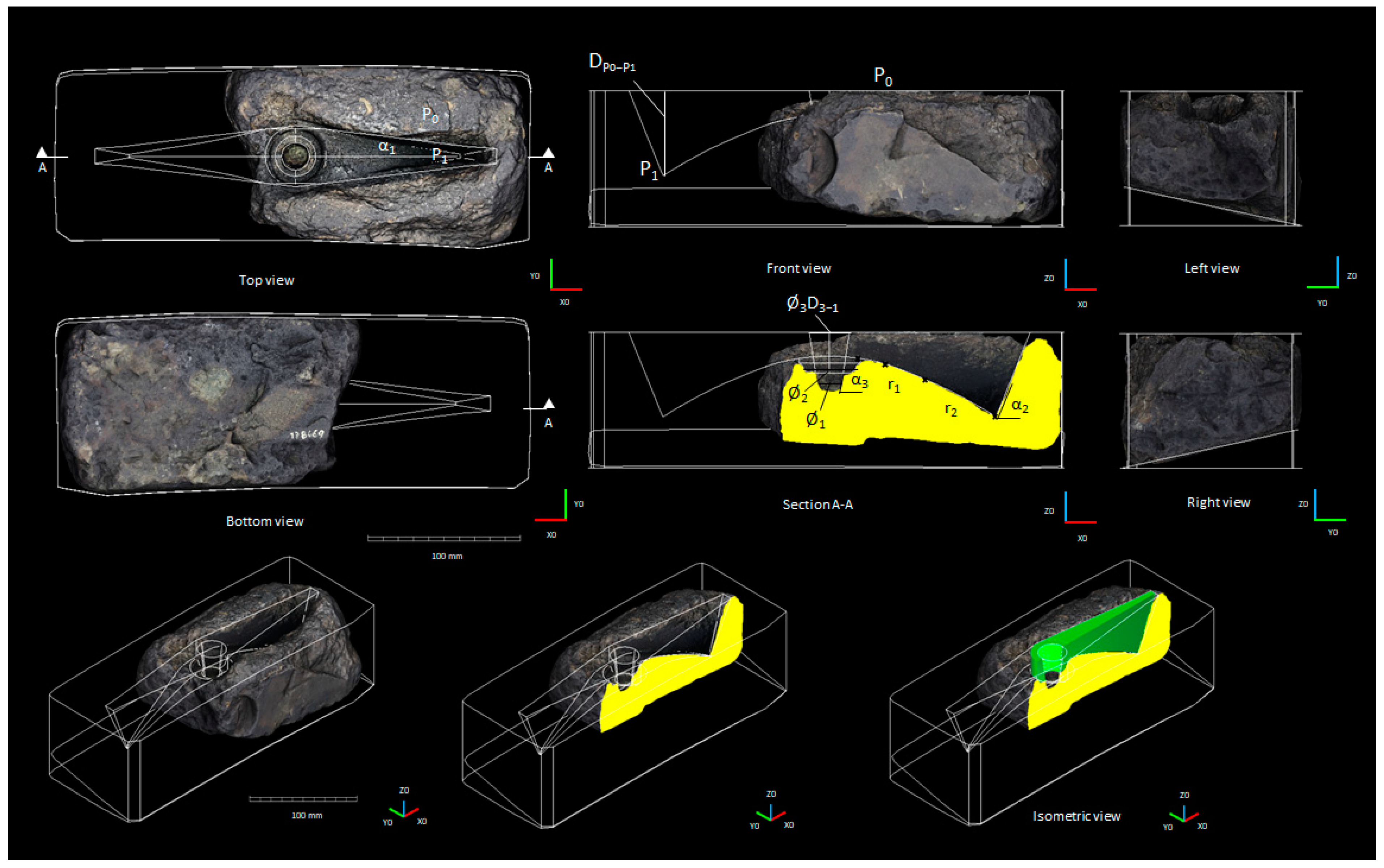
Finally, we report the results of the detailed morphometric analysis carried out on the 3D model of mould S1, which was the best preserved. Following the typological classification carried out during the archaeological study of this artefact [1], we made an integration by providing the characteristic data of the shapes present on the artefact and verified the hypothesis on the possible final bronze object. In the data sheets produced for this artefact, all the characteristic parameters taken from the 3D model are indicated (Figure 16, Table 9). From the longitudinal and cross sections, we obtained the geometrical limits of the casting mould. The processing of these data allowed us to create a geometric model of the whole axe, as assumed by the typological study (Figure 17). In addition, the morphometric analysis carried out on the frontal face X0Z0 of the artefact allowed us to compare the curvature of this carving with that of the lower part of the casting mould, highlighting a strong geometric correspondence.
The first fact that we wanted to examine during this study is related to the lithological nature of the moulds, attributed by archaeologists to the “steatitic type”, that is based fundamentally on the chromatic characteristics of the finds.
Our mineralogical–petrographic investigation revealed a predominantly chloritic composition of the stone artefacts, showing a strong analogy with the talc–chlorite outcrops observed in a vast area of Central Sardinia [19]. Starting from these assumptions, it seemed natural to ask whether the talc–chlorite materials were already known and used at the time of manufacture of the studied finds.
In particular, a close correlation emerges from the comparison between the macroscopic characteristics and the mineral–petrographic composition of the stone moulds and the rocks sampled from the outcrops in the district of Orani (Central Sardinia); the latter is very close to the discovery sites of most of the archaeological finds investigated. This preliminary investigation it allows us to state that the materials of these moulds are not of the “steatite type”, as previously assumed on the basis of macroscopic comparisons with other similar finds from the same Age.
In our study, we have also proposed a photogrammetric method with the best resolution for measuring the peculiar characteristics of this kind of artefacts, according to the maximum acceptable measurement error. We have analysed in detail the 3D models of the artefacts, highlighting the critical issues related to the quality of the captured images, the variability of the shape, and the color characteristics of the surfaces in relation to the accuracy of the digital models obtained. According to the reference literature for small-scale photogrammetic modelling, the accuracy of our 3D models is comparable and close to optical scanning systems modelling [4,6,7,15,19,21,22].
The results carried out with the morphometric analysis of the S1 mould allowed us to identify the original shape and dimension of the bronze axe through detailed parametric measurement of the 3D model. The processing of the 3D model to obtain the 2D drawings made it possible to emphasise, through additional measurements, other intrinsic characteristics not detectable or comparable through common macroscopic observation of the artefacts. The comparison between the internal shape of the S1 mould and the curved engraving on its front view face (X0Z0) allowed us to highlight a strong geometric correspondence. The engraved shape seems to be a kind of drawing used as a guide for the carving of the final casting mould.
4. Conclusions
The results presented in this paper demonstrate the potential of an integrated minero-petrographic and photogrammetric approach for the study of small archaeological artefacts and provide an effective tool for more in-depth analysis of future typological comparisons and provenance studies.
The results of the preliminary minero-petrographic investigation and the calculation of apparent specific weight derived from the morphometric analysis reveal the compositional homogeneity of the studied artefacts. These considerations allow us to assert that the stone moulds were probably made from the same lithotype. Based on these data, we performed the geoarchaeological survey for possible compatible raw materials, which was focused on the talc–chlorite bodies outcropping in the district of Orani (Central Sardinia). The minero-petrographic analysis of these materials showed the same mineral association of the five stone moulds. The five stone moulds studied are therefore all likely to have been produced in the Orani district, although one of them (N1) was found in a different area (Narbolia). This leads us to hypothesise a local production centre in the Orani district. However, the comparison with only one petrographic sample (taken from B1) does not allow us to define with certainty the precise location of the raw materials used to make these casting moulds. Further investigation of the nature of these stone moulds through a possible extension of the petrographic analysis to the other artefacts and a more detailed geoarchaeological survey may provide more reliable information on their provenance.
The morphometric analysis of the five stone moulds allowed us to identify their detailed dimensional parameters through 3D models using a local reference system. 2D orthoviews derived from the 3D models emphasised other intrinsic characteristics not detectable or comparable through common macroscopic observation of the artefacts.
The results of the accuracy check carried out on our digital models demonstrates that the error of the measurements is lower than the assumed maximum tolerance range 1:1000 ÷ 1:2000. The 3D reconstructions make it possible to analyse the artefacts down to the scale of extreme detail, with the advantage of saving time and money, with the goal of developing collaborations between scientists from different disciplines, even very distant from each other. Future developments of this multidisciplinary approach will be the further integration of photogrammetry as an analysis and measurement tool at different scales of investigation in the field of archaeology and cultural heritage.
Author Contributions
S.C., C.M. and P.V. conceived the integrated diagnostic photogrammetric methodology and contributed to the macroscopic analysis of the materials; S.C. and C.M. planned and carried out the experimental photogrammetric data acquisition; C.M. processed and interpreted the photogrammetric data; S.C. and P.V. planned and carried out XRD, petrographic analysis and geoarcheological survey; All the authors analysed and discussed the results, contributed to the manuscript drafting and revision. All authors have read and agreed to the published version of the manuscript.
Funding
This research received funding by the University of Cagliari (FIR 2020) and Regione Autonoma della Sardegna (GETHERE n. F71/17000190002).
Data Availability Statement
Not applicable.
Acknowledgments
We are very grateful to Alessandro Usai (Archaeological Superintendence of Cagliari and Oristano, Sardinia, Italy) for providing the stone moulds for this study. We wish also to thank Michal Jancosek, for supporting our research with the advanced photogrammetry software, RealityCapture.
Conflicts of Interest
The authors declare no conflict of interest.
References
- Usai, A. A proposito di alcune matrici nuragiche da Bidonì, Sorradile e Narbolia (OR). In Bronze Age Metallurgy on Mediterranean Islands: Volume in Honor of Robert Maddin and Vassos Karageorgis; Giumilia-Mair, A., Lo Schiavo, F., Eds.; Monographies instrumentum, 56; Editions Mergoil: Drémil-Lafage, France, 2018; pp. 377–391. ISBN 978-2-35518-083-5. [Google Scholar]
- Usai, A. Testimonianze Prenuragiche e Nuragiche nel Territorio di Narbolia. In Nurabolia-Narbolia; Zucca, R., Ed.; Una Villa di Frontiera del Giudicato di Arborea: Narbolia, Italy, 2005; pp. 21–57. [Google Scholar]
- Lo Schiavo, F. Le matrici e i crogioli della Sardegna nuragica. In Bronze Age Metallurgy on Mediterranean Islands: Volume in Honor of Robert Maddin and Vassos Karageorgis; Giumilia-Mair, A., Lo Schiavo, F., Eds.; Monographies instrumentum, 56; Editions Mergoil: Drémil-Lafage, France, 2018; pp. 195–238. ISBN 978-2-35518-083-5. [Google Scholar]
- Koutsoudis, A.; Vidmar, B.; Arnaoutoglou, F. Performance evaluation of a multi-image 3D reconstruction software on a low-feature artefact. J. Archaeol. Sci. 2013, 40, 4450–4456. [Google Scholar] [CrossRef]
- Sapirstein, P. A high-precision photogrammetric recording system for small artifacts. J. Cult. Herit. 2018, 31, 33–45. [Google Scholar] [CrossRef]
- Sapirstein, P. Accurate measurement with photogrammetry at large sites. J. Archaeol. Sci. 2016, 66, 137–145. [Google Scholar] [CrossRef]
- Jancosek, M.; Pajdla, T. Multi-view reconstruction preserving weakly-supported surface. In Proceedings of the IEEE Conference on Computer Vision and Pattern Recognition, Colorado Springs, CO, USA, 20–25 June 2011. [Google Scholar] [CrossRef]
- RealityCapture Software, Version 1.20.16813 Tarasque [CLI Software]. Epic Game Slovakia s.r.o., Slovakia. Available online: https://www.capturingreality.com (accessed on 30 September 2021).
- Schneider, C.T.; Sinnreich, K. Optical 3-D measurement systems for quality control in industry. Int. Arch. Photogramm. Remote Sens. 1992, 29, 56–59. [Google Scholar]
- Jin, T.; Dong, X. Designing and decoding algorithm of circular coded target. Appl. Res. Comput. 2019, 36, 263–267. [Google Scholar]
- Gajski, D.; Gasparovic, M. Applications of macro photogrammetry in archaeology. Int. Arch. Photogramm. Remote Sens. Spat. Inf. Sci. 2016, XLI-B5, 263–266. [Google Scholar] [CrossRef] [Green Version]
- Brown, D.C. Close-range camera calibration. Photogramm. Eng. 1971, 37, 855–866. [Google Scholar]
- Besl, P.J.; MacKay, N.D. A method fo registration of 3-D shapes. IEEE Trans. Pattern Anal. Mach. Intell. 1992, 14, 239–256. [Google Scholar] [CrossRef]
- CloudCompare, Version 2.11.3 [GNU GPL Software]. 2021. Available online: http://www.cloudcompare.org (accessed on 30 September 2021).
- Lerma, J.L.; Muir, C. Evaluating the 3D documentation of an early Christian upright stone with carvings from Scotland with multiples images. J. Archaeol. Sci. 2014, 46, 311–318. [Google Scholar] [CrossRef]
- Lague, D.; Brodu, N.; Leroux, J. Accurate 3D comparison of complex topography with terrestrial laser scanner: Application to the Rangitikei canyon (N-Z). ISPRS J. Photogramm. Remote Sens. 2013, 82, 10–26. [Google Scholar] [CrossRef] [Green Version]
- Henrikson, J. Completeness and total boundedness of the hausdorff metric. MIT Undergrad. J. Math. 1999, 1, 69–80. [Google Scholar]
- Tarini, M.; Cignoni, P.; Scopigno, R. Visibility based methods and assessment for detail-recovery. In Proceedings of the IEEE Visualization, 2003. VIS 2003, Seattle, WA, USA, 19–24 October 2003; pp. 457–464. [Google Scholar] [CrossRef] [Green Version]
- Fiori, C.; Grillo, S.M. Albite-chlorite and talc-chlorite deposits in metasedimentary and granitoid rocks of central Sardinia (Italy). Boletim Paranaense de Geociências 2002, 50, 51–57. [Google Scholar] [CrossRef] [Green Version]
- Delaunay, B. Sur la sphere vide. Bull. Acad. Sci. USSR Classe Sci. Mat. Nat. 1934, 7, 793–800. [Google Scholar]
- Galantucci, L.M.; Pesce, M.; Lavecchia, F. A stereo photogrammetry scanning methodology, for precise and accurate 3D digitization of small parts with sub-millimeter sized features. CIRP Ann. Manuf. Technol. 2015, 64, 507–510. [Google Scholar] [CrossRef]
- Galantucci, L.M.; Pesce, M.; Lavecchia, F. A powerful scanning methodology for 3D measurements of small parts with complex surfaces and sub millimeter-sized features, based on close range photogrammetry. Precis. Eng. 2016, 43, 211–219. [Google Scholar] [CrossRef]
Figure 1.
Sketch map of Sardinia and location of archaeological sites. 1—Santu Perdu; 2—Narbolia; 3—Sorradile.
Figure 1.
Sketch map of Sardinia and location of archaeological sites. 1—Santu Perdu; 2—Narbolia; 3—Sorradile.

Figure 2.
Views of the five stone moulds studied: (a) B1; (b) B2; (c) B3; (d) N1; (e) S1.

Figure 3.
(a) Schematic representation of the photogrammetric rig used in this investigation; (b) example of the DoF (12.4 mm) calculated for f/22 aperture, used for the largest find (S1).
Figure 3.
(a) Schematic representation of the photogrammetric rig used in this investigation; (b) example of the DoF (12.4 mm) calculated for f/22 aperture, used for the largest find (S1).
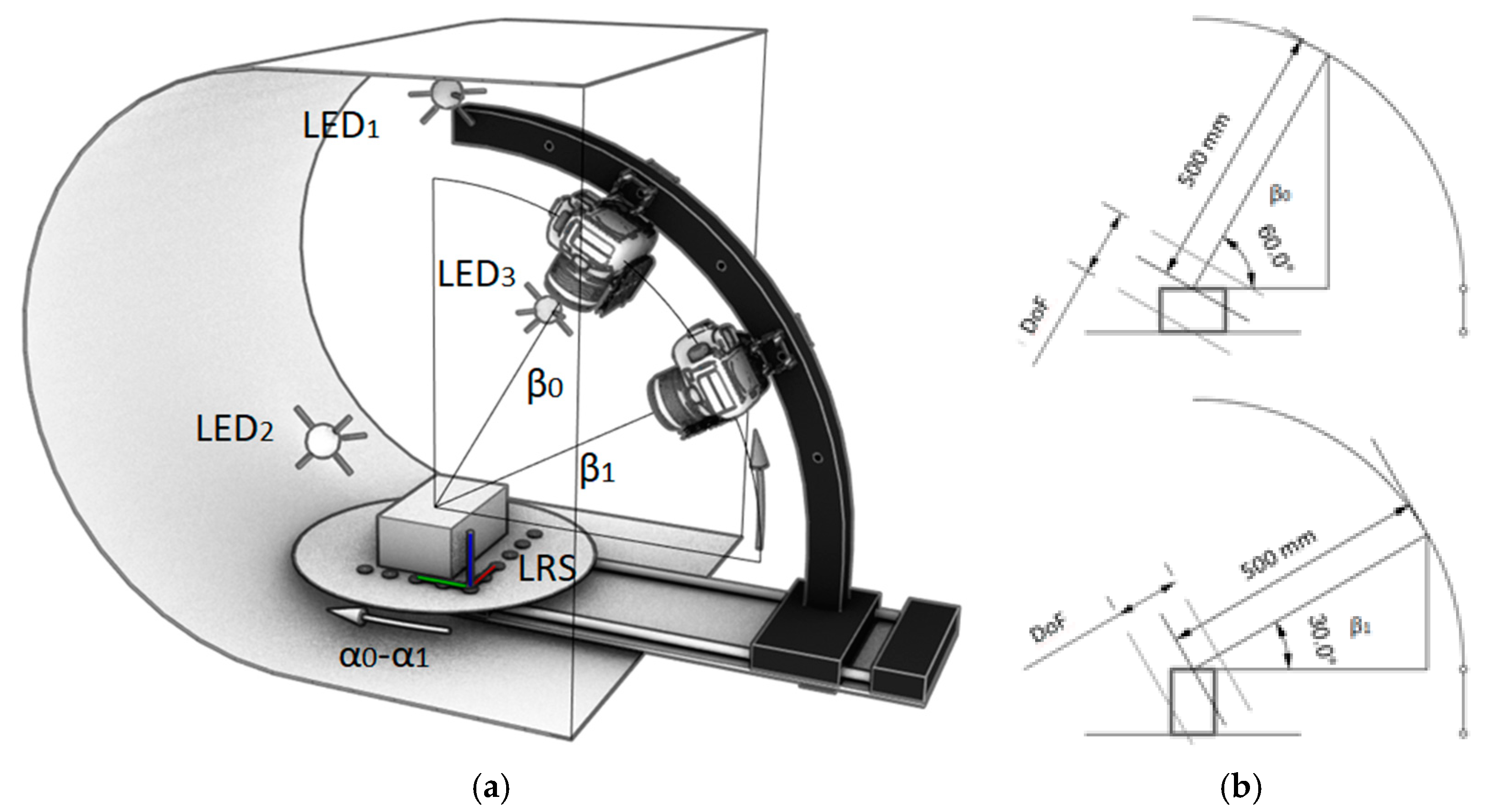
Figure 4.
Example of images captured for the find S1: (a) Original images; (b) Enhanced images with corrections. Quality improvement was achieved by adjusting RAW white balance, color correction, noise reduction and exposure compensation parameters.
Figure 4.
Example of images captured for the find S1: (a) Original images; (b) Enhanced images with corrections. Quality improvement was achieved by adjusting RAW white balance, color correction, noise reduction and exposure compensation parameters.
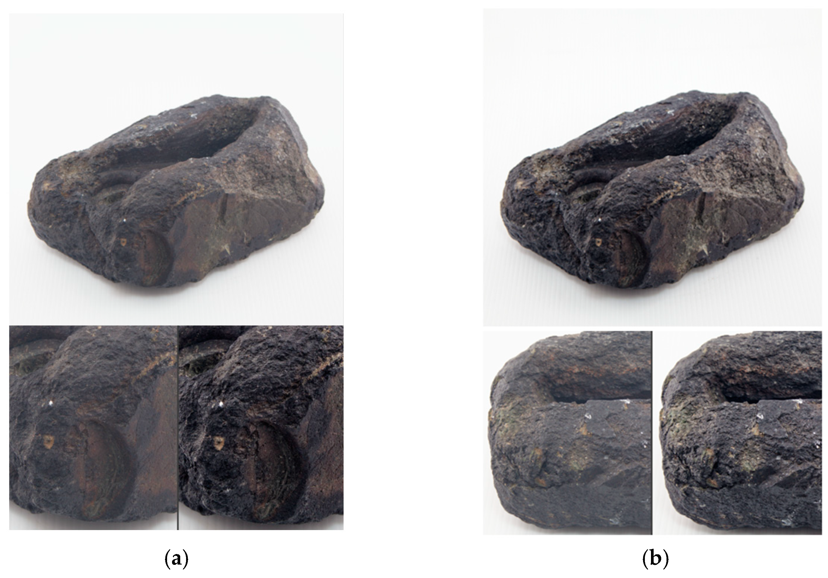
Figure 5.
Screenshots of Narbolia mould (N1) and reconstruction region (RR) with L-shape Reference System (LRS) on RC: (a) point cloud model, (b) textured model.
Figure 5.
Screenshots of Narbolia mould (N1) and reconstruction region (RR) with L-shape Reference System (LRS) on RC: (a) point cloud model, (b) textured model.

Figure 6.
XRD analysis of stone moulds Samples B1–B3. Cl = clinochlore; Qz = quartz; Alb = albite.
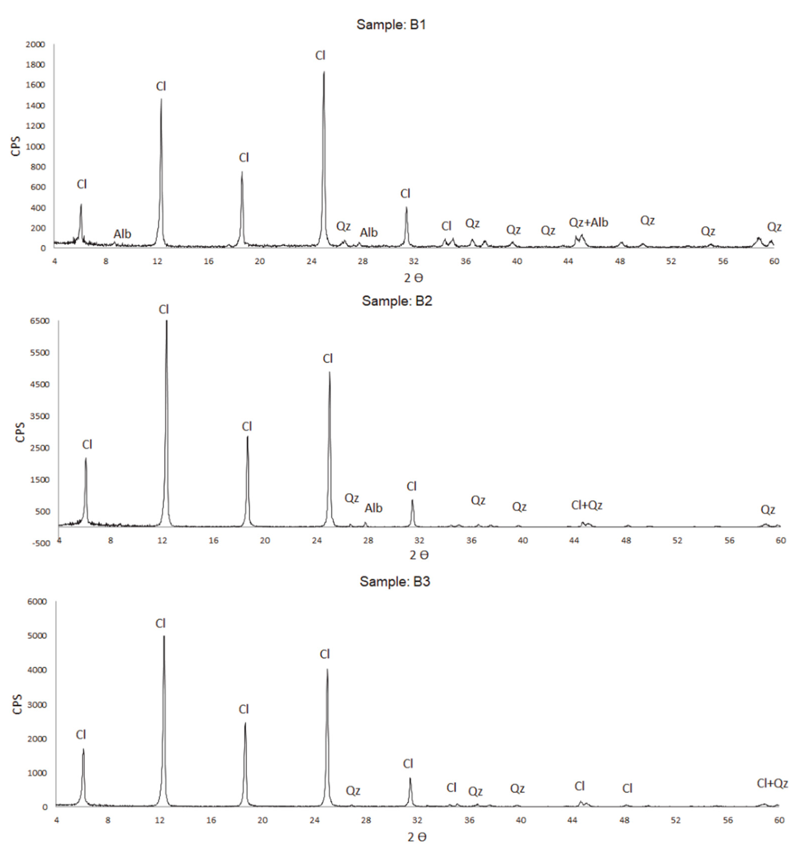
Figure 7.
XRD analysis of stone moulds Sample S1, Sample N1 and a compatible rock material (Sample O1). Cl = clinochlore; Qz = quartz; Alb = albite.
Figure 7.
XRD analysis of stone moulds Sample S1, Sample N1 and a compatible rock material (Sample O1). Cl = clinochlore; Qz = quartz; Alb = albite.
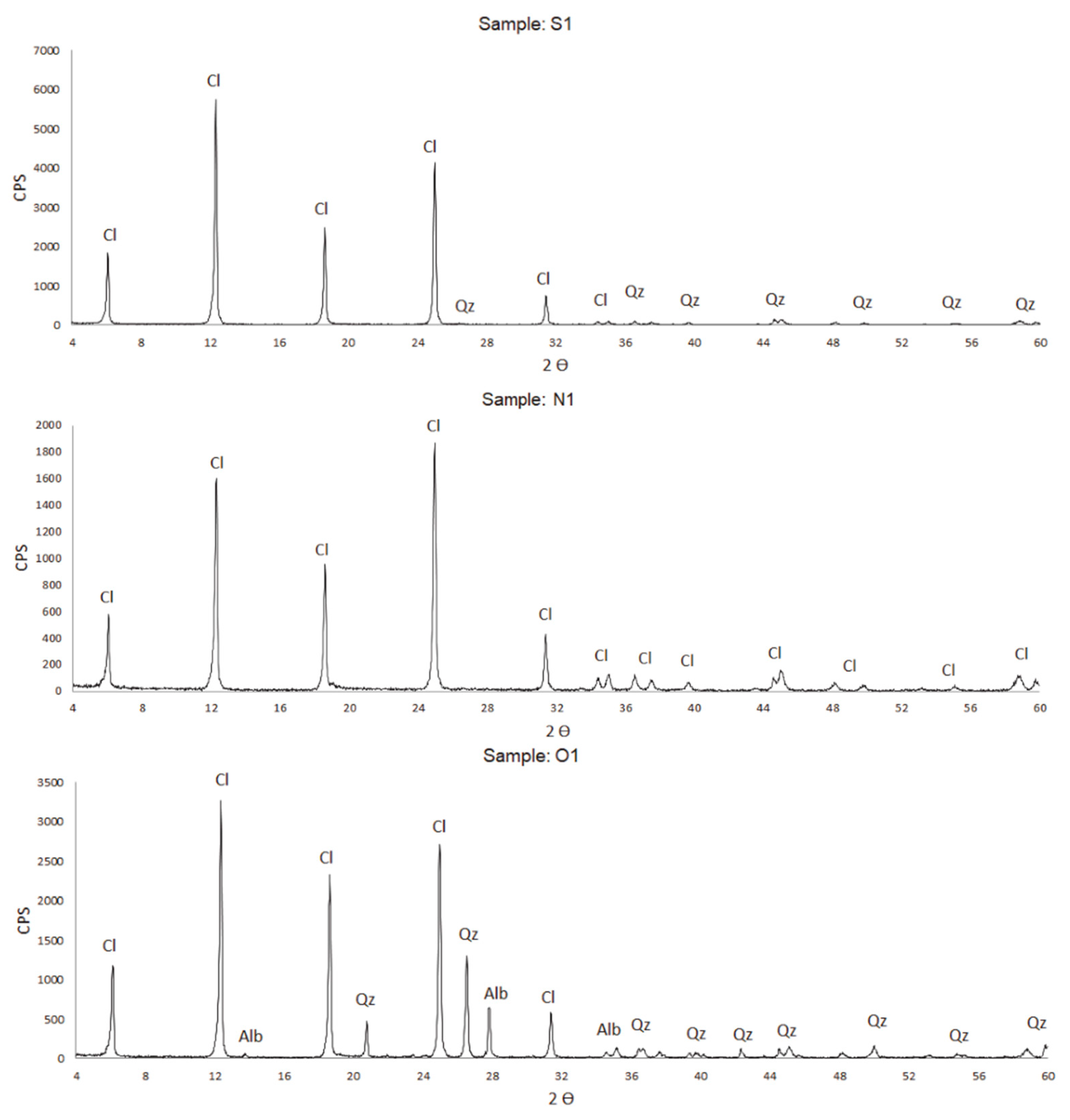
Figure 8.
Microphotographs of mould B1: (a) crossed nicols; (b) parallel nicols. O1 compatible material from the Orani district (Central Sardinia); (c) crossed nicols; (d) parallel nicols. Graphic scale = 1 mm.
Figure 8.
Microphotographs of mould B1: (a) crossed nicols; (b) parallel nicols. O1 compatible material from the Orani district (Central Sardinia); (c) crossed nicols; (d) parallel nicols. Graphic scale = 1 mm.
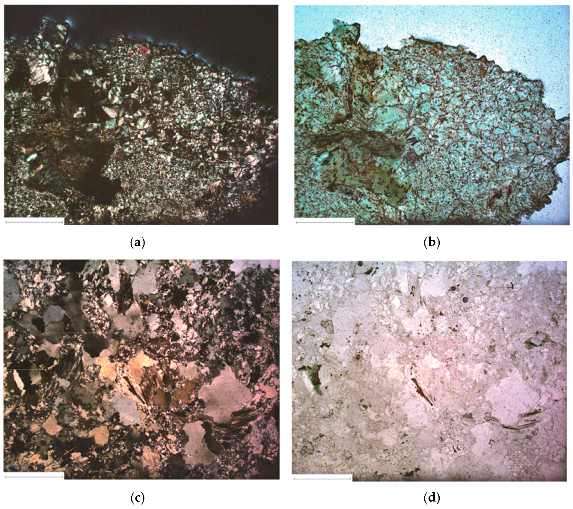
Figure 9.
Box-Plots showing the Q95 percentile (whiskers) of absolute distance errors (C2C distance and C2C-L local distance) among the 3D point cloud models in the 3D comparison after registration using the ICP method. Distance range was referenced to PCMS (Point Cloud minimum spacing).
Figure 9.
Box-Plots showing the Q95 percentile (whiskers) of absolute distance errors (C2C distance and C2C-L local distance) among the 3D point cloud models in the 3D comparison after registration using the ICP method. Distance range was referenced to PCMS (Point Cloud minimum spacing).
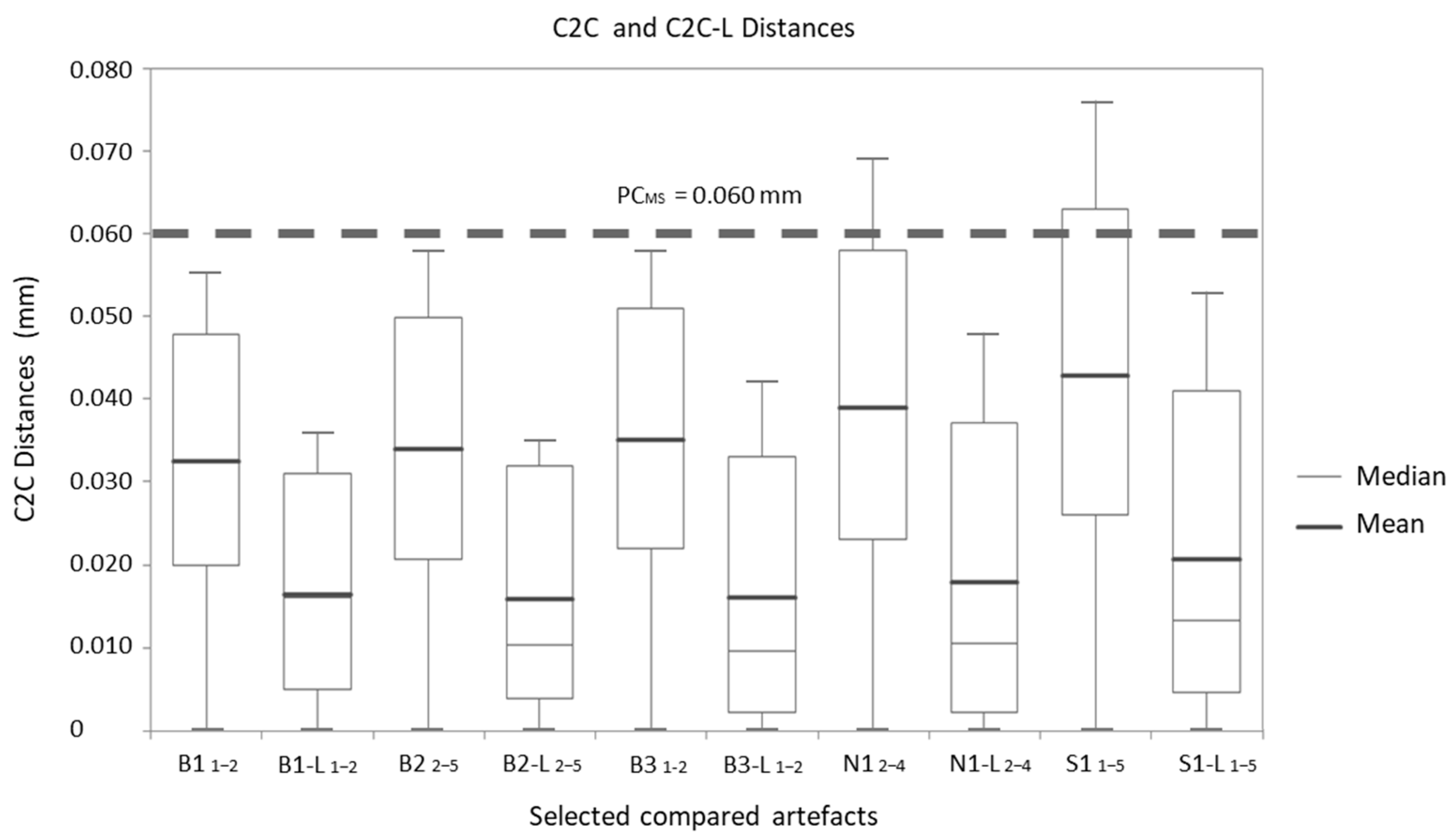
Figure 10.
Box-Plots showing the M+2SD (whiskers) of scalar field C2C-X, C2C-Y, C2C-Z among 3D point cloud models compared after registration with ICP method, referenced to PCMS = 0.060mm and T (tolerance limit).
Figure 10.
Box-Plots showing the M+2SD (whiskers) of scalar field C2C-X, C2C-Y, C2C-Z among 3D point cloud models compared after registration with ICP method, referenced to PCMS = 0.060mm and T (tolerance limit).

Figure 11.
Orthoviews from B1 3D model, with texture and Shade Vis Plug-in; visualization with CloudCompare software.
Figure 11.
Orthoviews from B1 3D model, with texture and Shade Vis Plug-in; visualization with CloudCompare software.

Figure 12.
Orthoviews from B2 3D model, with texture and Shade Vis Plug-in; visualization with CloudCompare software.
Figure 12.
Orthoviews from B2 3D model, with texture and Shade Vis Plug-in; visualization with CloudCompare software.

Figure 13.
Orthoviews from B3 3D model, with texture and Shade Vis Plug-in; visualization with CloudCompare software.
Figure 13.
Orthoviews from B3 3D model, with texture and Shade Vis Plug-in; visualization with CloudCompare software.
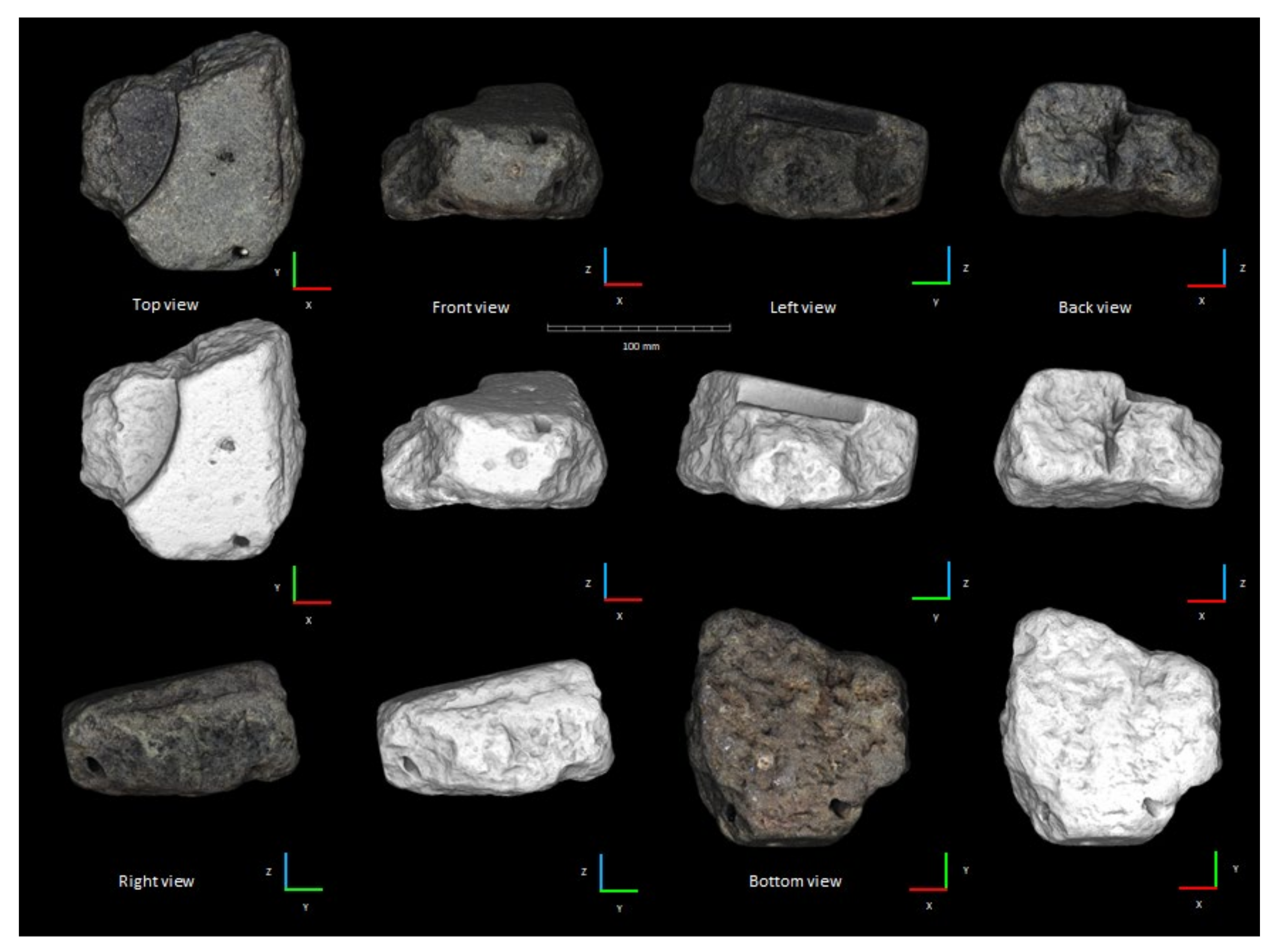
Figure 14.
Orthoviews from N1 3D model, with texture and Shade Vis Plug-in; visualization with CloudCompare software.
Figure 14.
Orthoviews from N1 3D model, with texture and Shade Vis Plug-in; visualization with CloudCompare software.
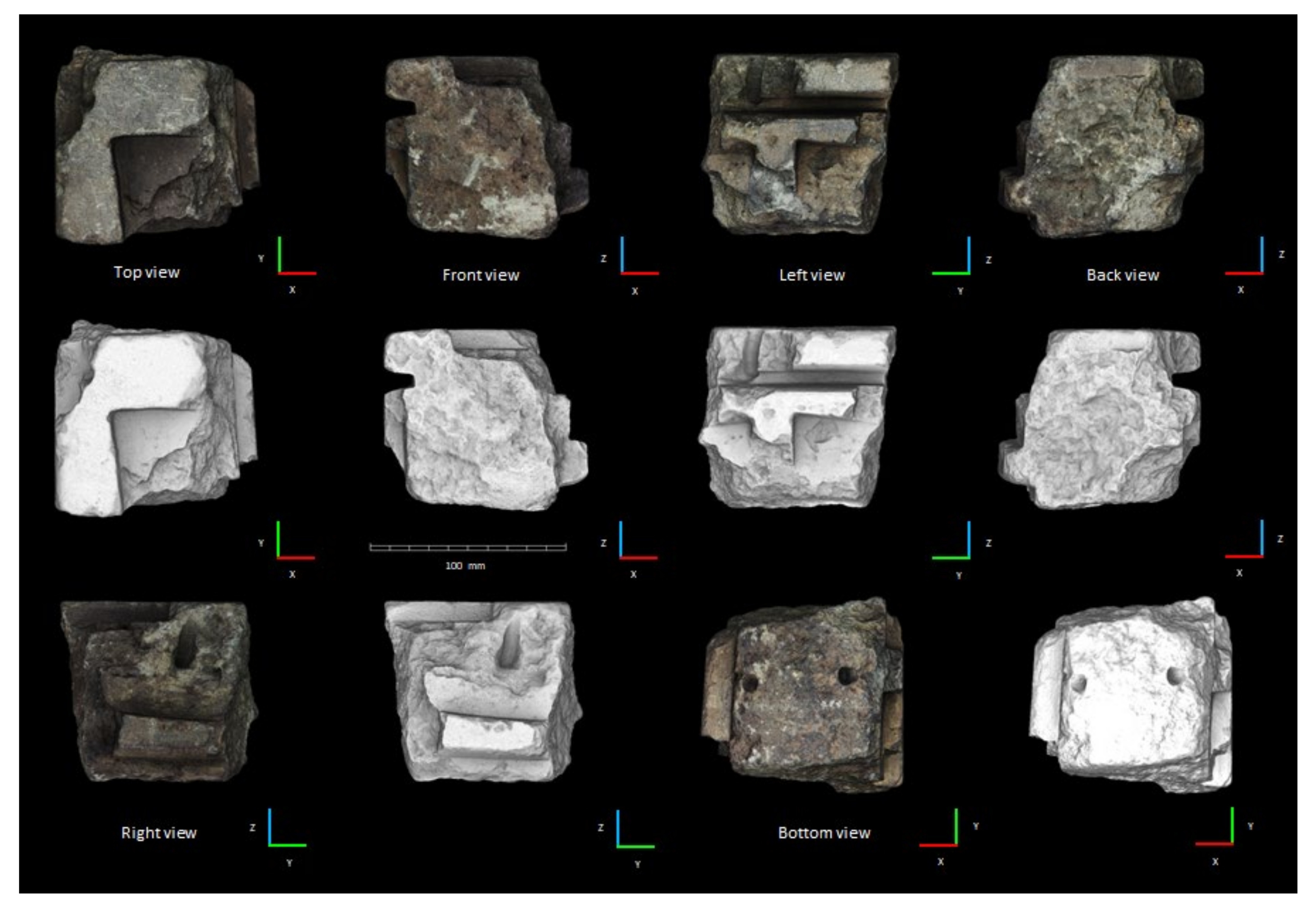
Figure 15.
Orthoviews from of S1 3D model, with texture and Shade Vis Plug-in; visualization with CloudCompare software.
Figure 15.
Orthoviews from of S1 3D model, with texture and Shade Vis Plug-in; visualization with CloudCompare software.
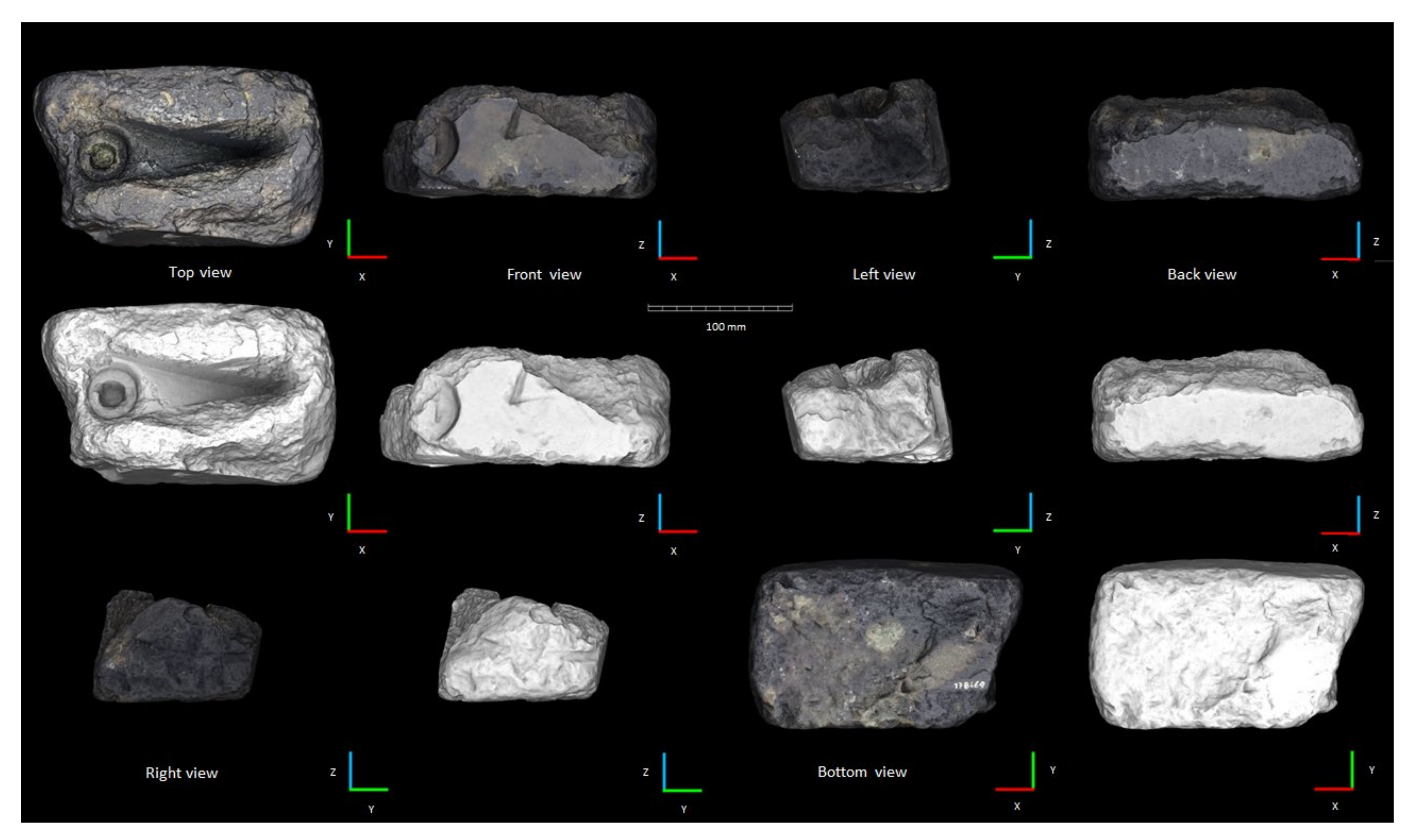
Figure 16.
Example of orthoviews, isometric views and sections of the Sorradile (S1) 3D model. Dimensional indicators and orientation of worked surfaces and holes on 3D model. DP0−P1 = mould depth; Dn = mould depth; Ø = diameter of circular shapes; Ømn = average diameter of the circular shape.
Figure 16.
Example of orthoviews, isometric views and sections of the Sorradile (S1) 3D model. Dimensional indicators and orientation of worked surfaces and holes on 3D model. DP0−P1 = mould depth; Dn = mould depth; Ø = diameter of circular shapes; Ømn = average diameter of the circular shape.

Figure 17.
Sorradile mould (S1 3D model): orthoviews, isometric views and sections and dimensional parameters of the mould, oriented according to the worked surfaces. Example of 3D geometric reconstruction of the original shapes and dimensional parameters of the mould (DP0−P1 = mould depth; Dn = mould depth; Ø = diameter of circular shapes; Ømn = average diameter of the circular shapes).

Table 1.
Dimensional characteristics and color (mean RGB values) of the archaeological finds studied.
Table 1.
Dimensional characteristics and color (mean RGB values) of the archaeological finds studied.
| Artefact | Length Max | Width Max | Height Max | External Color (RGB) | Mould Color (RGB) |
|---|---|---|---|---|---|
| (mm) | (mm) | (mm) | |||
| B1 | 100.8 | 75.7 | 48.1 | 61–59–56 | 68–60–54 |
| B2 | 95.0 | 114.7 | 65.1 | 53–54–52 | 45–45–43 |
| B3 | 124.6 | 133.2 | 76.2 | 88–89–93 | 35–36–34 |
| N1 | 111.7 | 104.5 | 95.3 | 85–76–62 | 104–91–71 |
| S1 | 201.9 | 125.5 | 83.8 | 109–109–113 | 60–59–64 |
Table 2.
Setting values for the Camera (Canon EOS RP) depending on the object dimension and maximum DoF.
Table 2.
Setting values for the Camera (Canon EOS RP) depending on the object dimension and maximum DoF.
| Artefact | Focal Length | Camera Tilt | Step Angle | Object Side | D | DoF | Aperture | n. Images |
|---|---|---|---|---|---|---|---|---|
| (mm) | (β) | (α) | (n) | (mm) | (mm) | ≥6 | ||
| B 1 * | 50 | 60 | 12 | 1 | 500 | 87 | f/16 | 10 |
| B 2 * | 50 | 60 | 12 | 1 | 500 | 87 | f/16 | 10 |
| B 3 * | 50 | 60 | 12 | 1 | 500 | 87 | f/16 | 10 |
| N1 * | 50 | 60 | 12 | 1 | 500 | 124 | f/22 | 10 |
| S1 * | 50 | 60 | 12 | 1 | 500 | 124 | f/22 | 10 |
| B 1 | 50 | 60 | 12 | 6 | 500 | 87 | f/16 | 180 |
| B 2 | 50 | 60 | 12 | 6 | 500 | 87 | f/16 | 180 |
| B 3 | 50 | 60 | 12 | 6 | 500 | 87 | f/16 | 180 |
| N1 | 50 | 60 | 12 | 6 | 500 | 124 | f/22 | 180 |
| S1 | 50 | 30 | 12 | 2 | 500 | 124 | f/22 | 60 |
| S1 | 50 | 30/60 | 7/12 | 2 | 500 | 124 | f/22 | 162 |
* First capture session with L-shaped reference system with codec targets (CPs) in place on the artefacts for calibration.
Table 3.
Alignment settings and reprojection errors calculated for all datasets with RC software.
| Artefact | Camera’s Count | Triangle’s Count | Point’s Count | Max Error (pix) | Median Error (pix) | Mean Error (pix) |
|---|---|---|---|---|---|---|
| B1 | 190 | 5.6 M | 2.8 M | 0.623999 | 0.185081 | 0.217189 |
| B2 | 190 | 8.7 M | 4.4 M | 0.623997 | 0.198011 | 0.229245 |
| B3 | 190 | 11.2 M | 5.6 M | 0.623962 | 0.195791 | 0.226403 |
| N1 | 190 | 15.2 M | 7.6 M | 0.623998 | 0.195359 | 0.226753 |
| S1 | 232 | 21.5 M | 10.8 M | 0.561598 | 0.184055 | 0.211238 |
Table 4.
Average distances (M) and standard deviations (SD) of C2C absolute distance errors of 3D comparisons, after ICP registration method.
Table 4.
Average distances (M) and standard deviations (SD) of C2C absolute distance errors of 3D comparisons, after ICP registration method.
| Compared | B1 | B2 | B3 | N1 | S1 | |||||
|---|---|---|---|---|---|---|---|---|---|---|
| C2C Distance | M (mm) | SD (mm) | M (mm) | SD (mm) | M (mm) | SD (mm) | M (mm) | SD (mm) | M (mm) | SD (mm) |
| 1–2 | 0.032 | 0.012 | 0.034 | 0.014 | 0.035 | 0.013 | 0.039 | 0.016 | 0.04 | 0.018 |
| 1–3 | 0.036 | 0.012 | 0.034 | 0.014 | 0.035 | 0.013 | 0.042 | 0.015 | 0.046 | 0.017 |
| 1–4 | 0.034 | 0.011 | 0.037 | 0.013 | 0.038 | 0.014 | 0.042 | 0.015 | 0.045 | 0.018 |
| 1–5 | 0.036 | 0.011 | 0.035 | 0.012 | 0.036 | 0.015 | 0.039 | 0.017 | 0.043 | 0.017 |
| 2–3 | 0.031 | 0.013 | 0.031 | 0.015 | 0.033 | 0.015 | 0.036 | 0.016 | 0.043 | 0.017 |
| 2–4 | 0.030 | 0.014 | 0.032 | 0.013 | 0.038 | 0.012 | 0.039 | 0.016 | 0.041 | 0.018 |
| 2–5 | 0.030 | 0.014 | 0.034 | 0.013 | 0.037 | 0.012 | 0.039 | 0.016 | 0.045 | 0.017 |
| 3–4 | 0.031 | 0.013 | 0.032 | 0.012 | 0.035 | 0.013 | 0.037 | 0.017 | 0.042 | 0.018 |
| 3–5 | 0.032 | 0.012 | 0.033 | 0.013 | 0.033 | 0.014 | 0.035 | 0.018 | 0.044 | 0.015 |
| 4–5 | 0.032 | 0.012 | 0.036 | 0.012 | 0.034 | 0.013 | 0.041 | 0.016 | 0.042 | 0.018 |
Table 5.
Average distances (M) and standard deviations (SD) of selected C2C and C2C-L local distance comparison (from 2D1/2 triangulation model): B1 1–2 = compared points cloud 1 and 2, …, S1 1–5 = compared points cloud 1 and 5.
Table 5.
Average distances (M) and standard deviations (SD) of selected C2C and C2C-L local distance comparison (from 2D1/2 triangulation model): B1 1–2 = compared points cloud 1 and 2, …, S1 1–5 = compared points cloud 1 and 5.
| Compared | C2C Distance | C2C Q95 | C2C-L Distance | C2C-L Q95 | ||
|---|---|---|---|---|---|---|
| M (mm) | SD (mm) | (mm) | M (mm) | SD (mm) | (mm) | |
| B1 1–2 | 0.032 | 0.012 | 0.055 | 0.016 | 0.011 | 0.036 |
| B2 2–5 | 0.034 | 0.013 | 0.058 | 0.016 | 0.011 | 0.035 |
| B3 1–2 | 0.035 | 0.013 | 0.058 | 0.016 | 0.012 | 0.042 |
| N1 2–4 | 0.039 | 0.016 | 0.069 | 0.018 | 0.017 | 0.048 |
| S1 1–5 | 0.043 | 0.017 | 0.076 | 0.021 | 0.018 | 0.053 |
Table 6.
Average distances (M) and standard deviations (SD) of C2C surface deviation analysis calculated with M±2SD on scalar fields C2C-X, C2C-Y, C2C-Z distances.
Table 6.
Average distances (M) and standard deviations (SD) of C2C surface deviation analysis calculated with M±2SD on scalar fields C2C-X, C2C-Y, C2C-Z distances.
| Compared | C2C-X | M ± 2SD | C2C-Y | M ± 2SD | C2C-Z | M ± 2SD | |||
|---|---|---|---|---|---|---|---|---|---|
| M (mm) | SD (mm) | (mm) | M (mm) | SD (mm) | (mm) | M (mm) | SD (mm) | (mm) | |
| B1 1–2 | 0.001 | 0.022 | 0.001 ± 0.044 | 0.003 | 0.023 | 0.003 ± 0.046 | 0.001 | 0.021 | 0.001 ± 0.042 |
| B2 2–5 | 0.001 | 0.022 | 0.001 ± 0.044 | 0.002 | 0.023 | 0.002 ± 0.046 | −0.003 | 0.020 | −0.003 ± 0.040 |
| B3 1–2 | 0.002 | 0.023 | 0.002 ± 0.046 | 0.003 | 0.022 | 0.006 ± 0.044 | 0.002 | 0.019 | 0.002 ± 0.038 |
| N1 2–4 | −0.003 | 0.025 | −0.003 ± 0.050 | −0.003 | 0.024 | −0.003 ± 0.048 | 0.001 | 0.024 | 0.001 ± 0.048 |
| S1 1–5 | 0.003 | 0.028 | 0.003 ± 0.056 | 0.004 | 0.028 | 0.004 ± 0.056 | 0.002 | 0.026 | 0.002 ± 0.052 |
Table 7.
Dimensional characteristics of the archaeological artefacts (X, Y, Z direction) calculated by CloudCompare software.
Table 7.
Dimensional characteristics of the archaeological artefacts (X, Y, Z direction) calculated by CloudCompare software.
| Artefact | X Length Max | Y Width Max | Z Height Max | Faces | Casting | Holes |
|---|---|---|---|---|---|---|
| (mm) | (mm) | (mm) | num. | num. | num. | |
| B1 | 100.696 ± 0.044 | 75.584 ± 0.046 | 47.976 ± 0.056 | 6 | 1 | 2 |
| B2 | 95.021 ± 0.044 | 114.746 ± 0.046 | 65.005 ± 0.040 | 6 | 3 | 0 |
| B3 | 124.507 ± 0.046 | 133.235 ± 0.044 | 76.102 ± 0.038 | 6 | 1 | 1 |
| N1 | 111.677 ± 0.050 | 104.586 ± 0.048 | 95.201 ± 0.056 | 6 | 7 | 3 |
| S1 | 201.938 ± 0.058 | 125.468 ± 0.056 | 83.905 ± 0.052 | 6 | 1 | 0 |
Table 8.
Characteristics of worked surfaces and volume variation of the 3D archaeological artefacts reconstructed in RC.
Table 8.
Characteristics of worked surfaces and volume variation of the 3D archaeological artefacts reconstructed in RC.
| Artefact | Weight (g) | Mean Volume (cm3) | Mean Volumetric Error (%) | Mean Specific Weight * (g/cm3) | Mean Specific Weight * (Kg/m3) |
|---|---|---|---|---|---|
| B1 | 469.38 | 176.85 | 0.070 | 2.654129 | 2654.13 |
| B2 | 1079.59 | 389.68 | 0.065 | 2.770460 | 2770.46 |
| B3 | 1660.46 | 601.14 | 0.062 | 2.762190 | 2762.19 |
| N1 | 1563.70 | 572.93 | 0.068 | 2.729289 | 2729.29 |
| S1 | 3066.95 | 1123.01 | 0.070 | 2.731021 | 2731.02 |
* Apparent specific weight.
Table 9.
Morphometric analysis through 3D model of S1 artefact.
| Artefact | X Length Max | Y Width Max | Z Height Max | Faces | Casting | Holes | Weight | Mean Volume |
|---|---|---|---|---|---|---|---|---|
| (mm) | (mm) | (mm) | num. | num. | num. | (g) | (cm3) | |
| S1 | 200.25 | 119.932 | 87.855 | 6 | 1 | 0 | 3066.95 | 1123.01 |
| Casting Mould | DP0−P1 | Øm1/D1 | Øm2/D2 | α1 | α2 | α3 | r1 (3pts.) | r2 (3pts.) |
| (mm) | (mm) | (mm) | (°) | (°) | (°) | (mm) | (mm) | |
| S1 | 55.38 | 16.32/13.01 | 34.43/5.89 | 80.9 | 68.4 | 81.3 | 146.6 | 336.25 |
| Cast Axe | X/2 Length max | Y Width max | Z Height max | X/2 Length min | Y Width min | Z Height min | Øm1 | Ø3/D1-3 |
| (mm) | (mm) | (mm) | (mm) | (mm) | (mm) | (mm) | (mm) | |
| S1 | 131.84 | 40.51 | 55.57 | 109.44 | 9.98 | 26.58 | 18.11 | 26.33/26.58 |
DP0−P1 = mould depth; Dn = mould depth; Ø = diameter of circular shapes; Ømn = average diameter of the circular shape n.
Publisher’s Note: MDPI stays neutral with regard to jurisdictional claims in published maps and institutional affiliations. |
© 2021 by the authors. Licensee MDPI, Basel, Switzerland. This article is an open access article distributed under the terms and conditions of the Creative Commons Attribution (CC BY) license (https://creativecommons.org/licenses/by/4.0/).
Share and Cite
MDPI and ACS Style
Cara, S.; Valera, P.; Matzuzzi, C. Morphometric Analysis through 3D Modelling of Bronze Age Stone Moulds from Central Sardinia. Minerals 2021, 11, 1192. https://doi.org/10.3390/min11111192
AMA Style
Cara S, Valera P, Matzuzzi C. Morphometric Analysis through 3D Modelling of Bronze Age Stone Moulds from Central Sardinia. Minerals. 2021; 11(11):1192. https://doi.org/10.3390/min11111192
Chicago/Turabian StyleCara, Stefano, Paolo Valera, and Carlo Matzuzzi. 2021. "Morphometric Analysis through 3D Modelling of Bronze Age Stone Moulds from Central Sardinia" Minerals 11, no. 11: 1192. https://doi.org/10.3390/min11111192
Note that from the first issue of 2016, this journal uses article numbers instead of page numbers. See further details here.