Measurement of 3D-Shape Preferred Orientation (SPO) Using Synchrotron μ-CT: Applications for Estimation of Fault Motion Sense in a Fault Gouge

Abstract

We propose a 3D-shape preferred orientation (SPO) measurement method of rigid grains using synchrotron micro-computational tomography (μ-CT). The method includes oriented sampling, 3D μ-CT imaging, image filtering, ellipsoid fitting, and SPO measurement. After CT imaging, all processes are computerized, and the directions of thousands of rigid grains in 3D-space can be automatically measured. This method is optimized for estimating the orientation of the silt-sized rigid grains in fault gouge, which indicates P-shear direction in a fault system. This allows us to successfully deduce fault motion sense and quantify fault movement. Because this method requires a small amount of sample, it can be applied as an alternative to study fault systems, where the shear sense indicators are not distinct in the outcrop and the fault gouge is poorly developed. We applied the newly developed 3D-SPO method for a fault system in the Yangsan fault, one of the major faults in the southeastern Korean Peninsula, and observed the P-shear direction successfully.

1. Introduction

The presence of fault planes under the ground can be used as the basis to study the stress field at the time of paleo-fault activation and is one of the biggest factors affecting the stability of the ground evaluated in civil engineering and geotechnical engineering [1]. In addition, a development step of the fault is essential to understanding the tectonic revolution history. Accordingly, various methods have been proposed to utilize the micro texture of the rock to understand the major deformation mechanism of the fault. For instance, Lattice Preferred Orientation (LPO) analysis of clay minerals using X-rays and Anisotropy of Magnetic Susceptibility (AMS) analysis using magnetic properties of minerals are effective methods to understanding fault activation history [2,3,4,5]. In particular, recent studies that measured and analyzed AMS of a matrix composed of clay minerals included in the fault zone report that AMS is mostly affected by magnetic minerals such as hematite, but clay minerals are aligned similarly to the fault slip plane [6]. However, their object minerals were mostly limited to clay minerals in matrix, and there are only a few results of the texture analysis of minerals for fault gouges that exist in the brittle deformation zone.

The fault gouge is a kind of fault rock that has undergone an incohessive brittle deformation process, and it has visible fragments of less than 30% [7]. Therefore, rigid fragments and ductile clay matrix surrounding it are distributed in the fault gouge. Studies on behavior of rigid particles, which are on a relatively ductile matrix, have been conducted for a long time in various ways [8,9,10,11]. According to previous studies, particles such as garnet or feldspar in the shear ductile deformation zone are aligned according to the direction of shear deformation through rigid body rotation [12]. In addition, the SPO of quartz particles present in various types of fault rocks in the brittle deformation zone has been investigated through 2D plane optical and microscopic observations and computational modeling [13,14]. SPO is a simple texture that can be investigated in a fault rock, but it requires a large amount of data in a limited sample. In addition, past research, in which the subject of investigation was limited to the 2D plane, was forced to focus on the analysis of specific plane.

Nevertheless, SPO can act as an indicator of the movement of faults in shallow deep environments through several assumptions: (1) relatively brittle grains exist in the isolated and rounded form in the ductile clay matrix and (2) grains almost maintain their shape during rotation and/or movement. Quartz is rotated in the ductile clay matrix according to the fault slip, and most grains are arranged along the P-shear direction of the fault slip plane (Figure 1a, [13]). The arrangement of grains with a large aspect ratio (>4) is almost parallel to slip plane [12]. In this way, we can infer the slip direction by comparing the direction of the 2D-SPO with that of the fault plane. However, the reliability of 2D-SPO analysis is questionable, because of the insufficient number of particles included in the microscopic observation. Also, it is difficult to apply 2D-SPO analysis to fault gouge where the fault zone is poorly developed. Furthermore, SPO measurements conducted on 2D planes do not completely represent the direction of grains distributed in nature. Regarding these problems, some previous studies attempted to apply 3D-SPO to fault systems to overcome the limitations of 2D-SPO and to investigate the spatial orientation. However, because 3D-SPO is expensive and time consuming, it is difficult to apply it to obtain a large amount of data.

To solve the aforementioned problems, micro-computational tomography (CT) imaging has been applied to various geology field [15,16,17,18]. The CT method can preserve the original sample, and a wide range of sample sizes can be measured. Recently, a research has been attempted to measure the shape of quartz, calcite, and pores in a strained shale through laboratory X-ray CT, and has been conducted on the strain difference given to rocks around fault zone [19]. However, unlike laboratory X-ray CT, when using a 3D imaging beam line installed in synchrotron, the energy level can be freely adjusted within a desired range to obtain a 3D image with better resolution. In this study, we attempted to obtain a high-resolution 3D μ-CT image of the fault gouge using a synchrotron accelerator by adjusting various factors such as wavelength and beam size. After the image filtering process, we attempted to automatize SPO measurement by coding the ellipsoid-fitting process of rigid grains and estimated the 3D fault motion sense quantitatively. Because the newly developed 3D-SPO method can automatically measure multiple rigid grains, this method can dramatically save time and improve the reliability of SPO results.

2. SPO Method Development

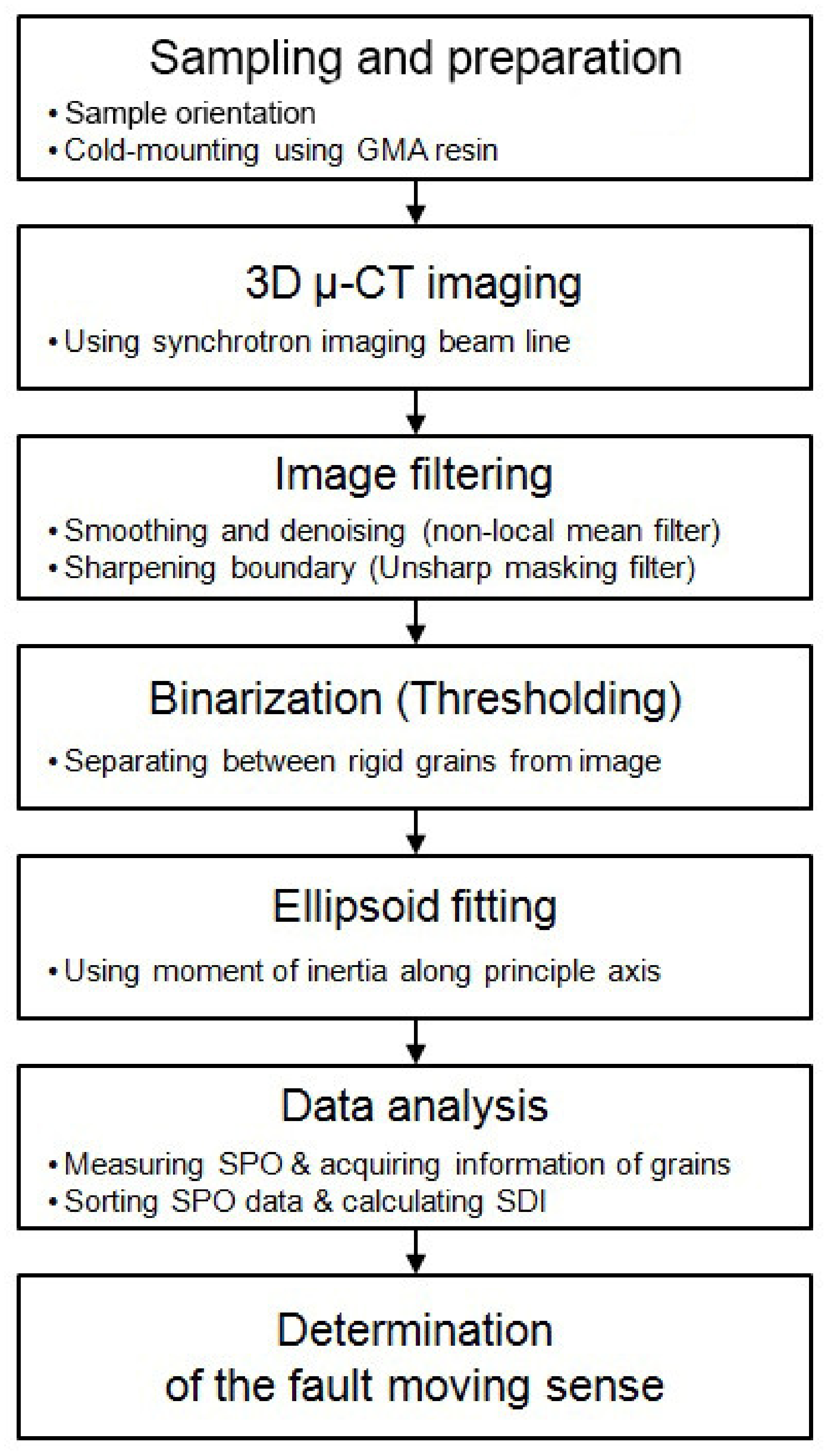
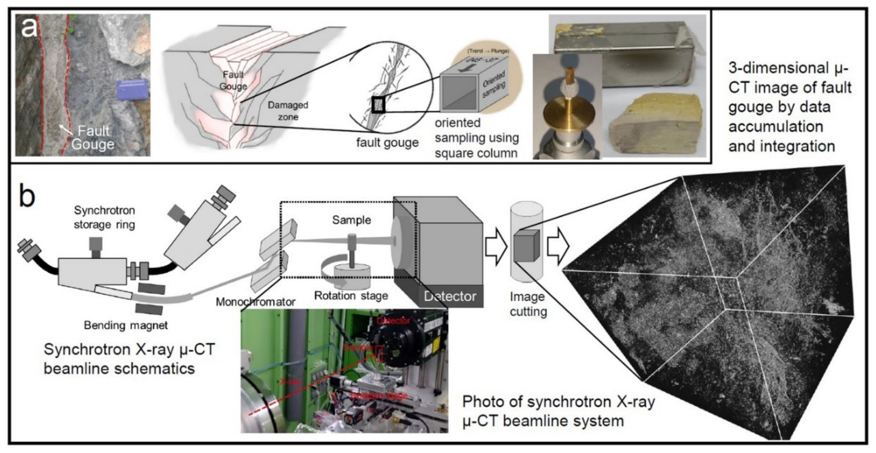
The newly developed 3D-SPO method comprises six steps—oriented sampling, 3D μ-CT imaging using the synchrotron beam line, image filtering and binarization, ellipsoid fitting, and SPO measurement. A flow chart of the steps is presented in Figure 2, and the details of each step are as follows.

2.1. μ-CT Imaging

We obtained μ-CT images at the beamline 6C Biomedical Imaging of the Pohang Light Source-II [20]. The beamline uses a multi-pole wiggler as its photon source and provides a monochromatic X-ray beam between 10 keV and 50 keV. For this experiment, we produced a 22-keV X-ray beam illumination using a double crystal monochromator based on silicon (111) reflection (DCM-V2; Vactron, Daegu, Korea). The specimen was mounted on an air-bearing rotation stage (ABRS-150MP-M-AS, Aerotech, Pittsburgh) 36 m from the source (Figure 3b). Behind the specimen, at a distance of 100 mm, an X-ray microscope was placed (Optique Peter, Lentilly, France) that comprised a 100-μm-thick CdWO4 scintillator facing the (010) direction (Miracrys LLC, Nizhny Novgorod, Russia), an objective lens of 4× magnification (UPLSAPO4X, Olympus, Tokyo, Japan), and a scientific CMOS camera (Zyla 5.5, Andor, Belfast, UK). The field of view (FOV) was 2.1 mm × 1.75 mm. For CT imaging, projections were acquired every 1.0° till a 180°rotation was complete. The exposure time was 0.5 s per projection.

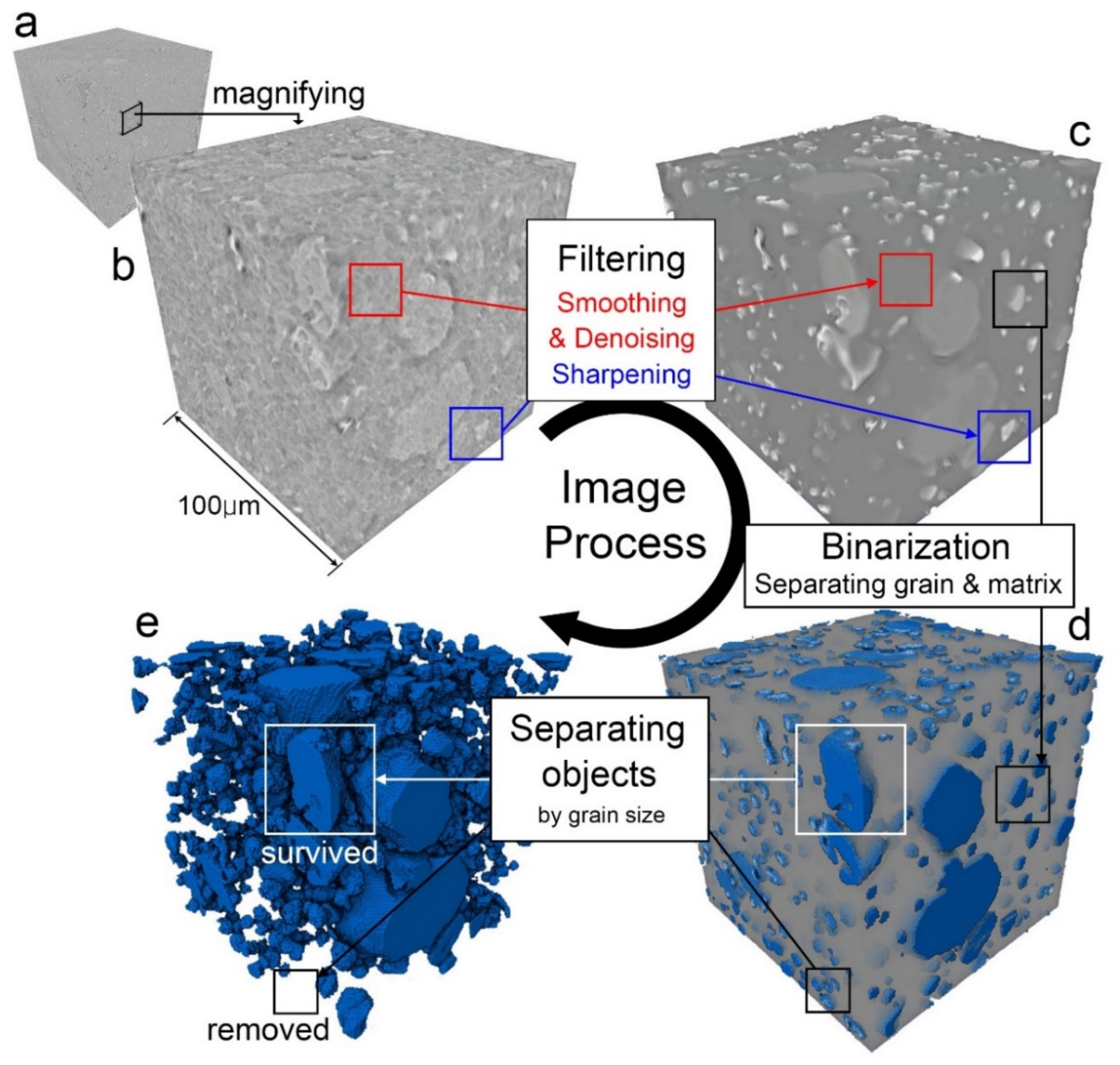
2.2. Image Processing and Ellipsoid Fitting

Images acquired for each rotated angle during CT imaging were converted into a stacked 2D-image form through reconstruction (Figure 3b). For image preprocessing, CT reconstruction was performed using Octopus 8.9 software (XRE, Gent, Belgium) that supported filtered-back projection (FBP) reconstruction. The 3D image, which was converted into a stacking type of cube-shaped pixels, had a size of 2238 × 2238 × 1865, and the size of each pixel was approximately 0.94 μm. The resulting 3D images were processed and analyzed using Amira 6.5 (Thermo Fisher Scientific, Hillsboro, OR, USA). Before the image filtering process, each 3D-CT image was cropped in a cubic shape (800 µm × 800 µm × 800 µm) at the center of each sample, which had low noise (Figure 4a). Several filtering processes were applied to allow easy differentiation between the grains and the matrix (or pore) in stacked 3D images. Among the various filters, smoothing and denoising filters were applied to remove noise, and a boundary sharpening filter was applied to clarify the boundary of the grains and the matrix (Figure 4b,c). In many cases, the filtering process was applied more than once, and the number of filtering times and type were performed depended on the type of sample (fault gouge, igneous rock, unconsolidated sedimentary rock, etc.). A non-local mean filter was used for denoising and smoothing effects and an unsharp masking filter was used for sharpening the boundary between the grains and the matrix (Figure 4c). In non-local mean filtering, small noises were removed, and the image was smoothened [21]. An unsharp masking filter is used to reclassify grain and matrix boundaries that are not easily distinguished because of excessive smoothing [22]. During the filtering process, the intensity range of the image is compressed compared to before processing. Finally, the intensity of the sample usually shows a distribution between 20 and 50 k.

The filtered images can be divided into grain, matrix, and pore, which are binarized in the next step. Binarizing the images involves visually comparing the original image and the binarized image and checking the grains by entering the appropriate boundary values (Figure 4d,e). Generally, among all components, grains have the highest intensity value and pores have the lowest intensity value. In this study, because SPO had to be measured by classifying only grains, image intensity was set by binarization by setting the intensity boundary value to classify grains. The standard intensity value that distinguishes the grains varied slightly depending on image. Therefore, it was better to visually compare the original image for each image (Figure 4d). This is because CT images measured by synchrotron show similar transmittance even though the mineral composition of each sample or the sample size is different. Therefore, it is better to set a different intensity for each image than to set one standard intensity for all samples. Additionally, small particles (<100 px) are not well processed with ellipsoid fitting or are difficult to separate even if noise is not deleted or grains are very small, which are problems faced during binarizing small particles (Figure 4e). When measurement was performed on all samples including 100 px or less, the SPO directions of most small ellipsoids were in the directions of the principal X-, Y-, and Z-axes. This is because tiny objects with volumes of several tens of pixels are changed to simple ellipsoids with major axes in the direction of the X-, Y-, and Z-axes. Therefore, all grains with a volume less than the specific size (100 px in this study) in the binarized image were deleted. In addition, cut grains in the edge of the image were ignored in the analysis.

To estimate the orientation of each grain, the ellipsoid-fitting method developed which was adopted and be appropriate to fit an irregularly shaped object into ellipsoid [23]. By measuring the length of the x-, y-, and z-axes and the directions of the well-matched ellipsoid, the information of the aspect ratio (c/a), anisotropy (1-a/c), elongation (b/c), flatness (a/b), and the orientation of each axis can be obtained (Figure 5). Fitting was performed for the binarized images using MATLAB code modified from the code of Kang et al. [23]. First, the code was developed assuming an ellipsoid with a volume of the object and to determine the length (a, b, c) of the principle axes (x, y, z) with the vector component and their orientations. Therefore, a covariance matrix (1) with a second moment μ value (2) was constructed.

$${\displaystyle \sum }_{}^{}=\left[\begin{array}{ccc}{\mathsf{\mu }}_{200}& {\mathsf{\mu }}_{110}& {\mathsf{\mu }}_{101}\\ {\mathsf{\mu }}_{110}& {\mathsf{\mu }}_{020}& {\mathsf{\mu }}_{011}\\ {\mathsf{\mu }}_{101}& {\mathsf{\mu }}_{011}& {\mathsf{\mu }}_{002}\end{array}\right]={\mathrm{V}}_{\mathrm{u}}{\mathrm{DV}}_{\mathrm{u}}{}^{\mathrm{T}}=\left[{\mathsf{\nu }}_{\mathrm{a}} {\mathsf{\nu }}_{\mathrm{b}} {\mathsf{\nu }}_{\mathrm{c}}\right]\left[\begin{array}{ccc}{\mathsf{\lambda }}_1& 0& 0\\ 0& {\mathsf{\lambda }}_2& 0\\ 0& 0& {\mathsf{\lambda }}_3\end{array}\right]\left[\begin{array}{c}{\mathsf{\nu }}_{\mathrm{a}}\\ {\mathsf{\nu }}_{\mathrm{b}}\\ {\mathsf{\nu }}_{\mathrm{c}}\end{array}\right]$$

(1)

$${\mathsf{\mu }}_{\mathrm{pqw}}=\frac{1}{\mathrm{n}}{\displaystyle \sum }_{\mathrm{i}=1}^{\mathrm{n}}{({\mathrm{x}}_{\mathrm{i}}-\overline{\mathrm{x}})}^{\mathrm{p}}{({\mathrm{y}}_{\mathrm{i}}-\overline{\mathrm{y}})}^{\mathrm{q}}{({\mathrm{z}}_{\mathrm{i}}-\overline{\mathrm{z}})}^{\mathrm{w}}$$

(2)

${\mathrm{V}}_{\mathsf{\mu }}$ is the unit vector of the principal axes, ${\mathsf{\lambda }}_1$, ${\mathsf{\lambda }}_2$, and ${\mathsf{\lambda }}_3$ are moments of inertia along the principal axes, and ${\mathsf{\nu }}_{\mathrm{a}}$, ${\mathsf{\nu }}_{\mathrm{b}}$, and ${\mathsf{\nu }}_{\mathrm{c}}$ are matrix elements that represent the directivity of ellipsoids orthogonal to one another.

In addition, assuming the volume factor S as shown in Equation (3) below, the length of each major axis is calculated to be $\mathrm{a}=\mathrm{S}·{\mathsf{\lambda }}_1$, $\mathrm{b}=\mathrm{S}·{\mathsf{\lambda }}_2$, and $\mathrm{c}=\mathrm{S}·{\mathsf{\lambda }}_3$ [23].

$${\mathrm{S}}^3=\frac{3}{4}· \frac{\mathrm{V}}{4\mathsf{\pi }·{\mathsf{\lambda }}_1·{\mathsf{\lambda }}_2·{\mathsf{\lambda }}_3}$$

(3)

By coding the equations, we can make the best-fit ellipsoid for each rigid grain and can measure the length (a, b, c) and the orientation (x, y, z-axis direction, V_a, V_b, V_c) for the ellipsoid automatically.

2.3. Data Analysis

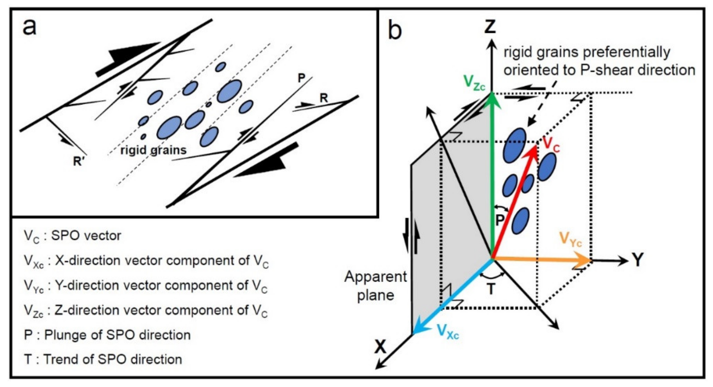
2.3.1. SPO Measurement

The data obtained from each grain through ellipsoid fitting are the length (a, b, c) and the orientation (especially explained about V_c in Figure 1b). We rearranged the whole data by the size (c), volume, and ellipsoid volume(4πabc/3), and the aspect ratio (c/a), which are crucial to interpret SPO results. The orientation (V_c) of the grain can be expressed by the direction vectors (Vx_c, Vy_c, Vz_c), which can be determined by measuring the trend (T), which is the rotated angle to the X axis in the XY plane, and the plunge (P), which is the angle between V_c and Z-axis (Figure 1b). In practice, T and P values are apparent values (T_a, P_a) measured with respect to reference plane. Therefore, by rotating these values using the orientation data of the sample, the real V_c direction (T_o, P_o) can be obtained. The T_o and P_o values of the target grains are plotted on an equal-area stereo-net with 5-degree intervals using MATLAB to present the distribution. The virtual measurement result of the SPO is shown in Figure 6a as an example, which shows how to display the fault plane (45 → 130) and the SPO (110 → 30) grains on the 2D stereo-net plane. In the same way, the ellipsoid’s middle axis (b, V_b) and minor axis (a, V_a) were also investigated and plotted on a stereo-net. The internal angle (θ) between the tomographic plane and the SPO direction can also be obtained through the dot product of the vector. To consider the factors affecting the results, the overall SPO data were plotted on stereo-net after dividing into given size fraction (<5, 5–10, 10–15, >15 μm), given volume fraction (<100, 100–1000, 1000–10,000, >10,000 μm³), and given aspect ratio (<1.5, 1.5–2, 2–3, >3). All data sorting processes were automated by MATLAB-based coding.

2.3.2. SPO Distribution Index

The distribution densities of directions of SPO values were presented as a contour map image. There are several indexes to express the distribution of 3D orientation such as Orientation Distribution Function (ODF), multiples of random distribution (m.r.d.), and mean tensor [24,25,26]. However, in the case of ODF containing a volume factor, there is a problem in that the weight is differently calculated for each grain. In addition, m.r.d. can express the relative distribution well through normalizing, but only presents quantitative values for densest points. Here we suggest an SPO distribution index (SDI) that can express the distribution density of SPO results quantitatively. The SDI indicates how the SPO data are scattered from the reference point, which is the most frequent direction. SDI is simply expressed as follows:

$$\mathsf{\gamma } =\frac{{\mathrm{X}}_{\mathsf{\phi }}}{{\mathrm{X}}_{\mathrm{T}}}\times 100\left(\%\right)$$

(4)

$${\mathrm{SDI}}_{\mathsf{\gamma }} = \mathsf{\phi }$$

(5)

${\mathrm{SDI}}_{\mathsf{\gamma }}$ represents the maximum value of the angle between the γ% of grains surveyed and the most dense point. $\mathsf{\phi }$ has a value between 0 and 180° and is the angle between the direction which has the largest frequency (the densest point) and the direction of the major axis of the target grain. ${\mathrm{X}}_{\mathsf{\phi }}$ is the number of objects in the direction of the major axis placed under the spatial angle of $\mathsf{\phi }$, and ${\mathrm{X}}_{\mathrm{T}}$ is the total number of objects. Therefore, the value of SDI ranges from 0 to 180°, and it determines the distribution density, i.e., how many datapoints among the total are arranged in the corresponding direction. In addition, the distribution density of SPO can also be presented simply using SDI values with different γ values. The higher the SDI value for given same γ-values is, the more scattered the directions (V_c) of the z-axes of the grains are, whereas the lower the SDI is, the more concentrated the arrangement of grains in a specific direction is.

3. Application of the 3D- SPO Method for a Fault Gouge Sample

3.1. Sample Preparation

The gouge sample was collected from a outcrop of Yangsan fault zone, which is one of the largest fault zones in the southeastern parts of the Korean Peninsula and has the longest and most prominent linear structure in the NNE direction of strike [27,28,29]. The sampling site (BK) is located in the northern part of the Yangsan fault, which penetrates through the fault core with a typical fault gouge. The fault zone is composed of a core zone (9−10 m in thickness) and surrounding damage zones (>200 m in thickness) [30]. In the fault core zone, lens shaped rock fragments of several centimeters to one meter in size appear, indicating a dextral sense of shear. Most clay minerals contained in the matrix are illite and chlorite, and some smectite is also present [30]. Sim et al. determined the fault activation ages were 20 and 26–28 Ma using the Illite age analysis (IAA) [31]. The fault plane observed in the outcrop stands vertically, and the direction of the fault plane is measured as N45° E 85° SE. In the fault core zone, the sample was taken from the fault gouge, and it is blue-grey colored and less than 50 cm wide.

To obtain samples for the experiment, the iron core was inserted into a fault gouge using a hammer, and then the strike and dip direction of the inserted surface was measured (Figure 3a). Before the sample was taken out, the strike direction of the injected iron core was marked. The collected samples were sealed during transport from the field to the laboratory, where the samples were dried for more than 24 h. Cold-mounting was performed using glycol methacrylate (GMA) resin which has similar viscosity with water at room temperature, because it was difficult to maintain the shape of the sample near the unconsolidated state by making slabs or thin sections. A GMA resin was used to solidify the sample at 60 °C under vacuum. For some samples, the cold-mounting process was repeated several times to fabricate a complete solid form of the specimen with the resin penetrating deep into the pore cavity. After cold-mounting was completed, the sample was cut into a size of 1 mm × 1 mm × 2 mm.

3.2. SPO Data of Fault Gouge Sample

μ-CT images of the fault gouge were obtained using the synchrotron beam line of the Pohang Light Source-II [20]. After image filtering for the μ-CT image, 3D-SPO estimation was performed by measuring the length (a, b, c) and direction vector (V_a, V_b, V_c) for the ellipsoid-fitted grains of 7636 particles. The 3D-SPO results of major axis were plotted with red color on the stereo-net with 5-degree intervals. In addition, the results of measuring the direction of the middle axis and minor axis of the ellipsoid are shown together in blue and green on the stereo-net, respectively (Figure 6b). Examples of data are shown in

Table 1. Measurement examples after ellipsoid fitting for 3D μ-CT images of the fault gouge sample.

N	Length of Axis			Direction Vector of z-Axis (Vc)			Trend and Plunge of Direction of z-Axis (Vc)				Angle
	a	b	c	Vxc	Vyc	Vzc	Ta	Pa	To	Po	θ
1	3.28	4.18	6.18	0.686	0.147	0.713	258	45.5	21.2	26.0	23.7
2	2.11	2.94	3.28	0.603	−0.796	0.052	323	57.6	250	45.6	20.8
3	3.41	4.57	5.68	−0.406	−0.906	0.122	24.1	7.03	213	12.3	10.6
4	3.57	4.09	9.05	0.229	0.961	0.157	193	9.06	50.9	6.80	5.3
5	1.87	5.29	9.79	0.415	0.742	0.527	209	31.8	60.2	21.6	11.9
…
7632	2.00	3.56	10.7	−0.075	−0.890	0.449	4.80	26.7	99.9	61.7	17.8
7633	3.72	9.49	12.7	0.237	0.601	0.763	202	49.8	12.6	20.7	31.6
7634	3.16	3.97	6.33	−0.246	−0.951	0.190	14.5	10.9	30.6	14.6	14.8
7635	2.30	2.95	8.45	−0.526	−0.245	0.814	66.0	54.5	99.3	23.6	44.5
7636	3.08	4.81	6.03	0.967	−0.142	0.213	278	12.3	248	67.0	13.4

T_a, P_a: Trend and plunge of the apparent direction of the z-axis (V_c); T_o, P_o: Trend and plunge of the restored original direction in which grains existed; θ: The angle between the fault plane and the z-axis of the grain.

. The grain size (c), which is the length of the z-axis of the fitted ellipsoid, ranged from 3.2 to 82.4 μm, and the grains of 85% have less than 10 μm sized. As the grain size increased, the number of grains tended to dramatically decrease. The range of the aspect ratio (c/a) is various, but the numbers 2–3 and >3 are the greatest. More detailed information of the investigated grains, such as anisotropy, flatness, elongation, graph of aspect ratio to grain size, and Scanning Electron Microscopy (SEM) images is given in Supplementary Materials (Figure S1–S3). SPO results were presented as a contour map on the stereo-net (Figure 6b and Figure 7). The point of the highest SPO density distribution was found to be 028 → 24 and has 17.0 of SDI₂₀ values. Various SDI examples with γ-values varying from 10 to 50 with 10 intervals for the 3D-SPO results are presented in Supplementary Materials Table S1. The SDI₂₀ values are presented on the contour plot to show the degree of distribution of the SPO results (Figure 6b). Finally, the angle (θ) between the fault plane and SPO direction was calculated from the dot product of the vector to verify whether it corresponds to the P-shear direction of the fault plane (Table 1).

The 3D-SPO results were classified into several groups by grain size, volume, and aspect ratio. the contour plots of each results are separately presented in Figure 7. The directions of the densest points for the each SPO data by grain size appeared in the order 028 → 22, 029 → 22, 023 → 20, and 025 → 22, with an SDI₂₀ value of almost 20 (Figure 7a–d). The directions were similar to the overall direction (028 → 22) as shown in Figure 6b, whereas the SDI₂₀ values were larger than the overall value (17.0). The directions of the densest points for the each SPO data by grain volume appeared in the order 030 → 24, 025 → 23, 026 → 23, and 022 → 20, with an SDI₂₀ value of 16 to 21 (Figure 7e–h). For the SPO data by each aspect ratio, the directions of the densest point are different and range from 018 → 14 to 030 → 29 (Figure 7i–l). These results were also slightly different; the overall direction is 028 → 24, and the SDI₂₀ values are approximately 20.

4. Discussions

4.1. SPO Data Interpretation and Implication

In this study, we successfully obtained 3D-SPO results from synchrotron μ-CT images. This developed 3D-SPO method allowed us to investigate the hidden vertical displacement of the strike-slip fault and the unmeasurable horizontal displacement of the vertical fault in the millimeter and micrometer scales. The SPO results of the middle and minor axes appeared scattered on a plane perpendicular to the SPO results of the major axes. Relatively, the data in the middle axis showed a dense form at two points, and these results, along with the characteristics of grains included in Supplementary Materials, could be considered as further research topics. On the other hand, we tried to identify the factors controlling SPO results. The case study showed that the spatial distribution of SPO looks more dispersed as grain sizes increased (Figure 7a–d). In particular, for the grains of sizes of <5 μm (2834) and 5 to 10 μm (3652), the SPO results were radially well-distributed on the contour plot (Figure 7a,b), whereas the contour plots of grains >15 μm (327) were relatively irregular (Figure 7d) with no distinct changes in the SPO direction. This could have been caused by the abundance of the size fractions of the target fault gouge. Although it was analyzed as above in the data classified by grain size, when the sufficient SPO data were collected, the difference in the tendency of the direction in each grain size was not large. This can also be confirmed in the SPO data classified by volume. The total SPO data is well matched the case of 100–1000 μm³ (5860) where most of the data is concentrated (Figure 7f). However, the other three cases, which have little data, have a larger SDI value or even some scattering points (Figure 7e). Therefore, the results of analysis of the contour plot and SDI distribution by particle size effect show that when studies are conducted on a small number of particles, the SPO data may be inaccurate. As a result, if multiple particles are included, regardless of particle size, the accuracy and precision of SPO results can be improved. As the SPO results were classified by aspect ratios, all results showed a similar direction for grains with similar SDI values, except for aspect ratios <1.5 (Figure 7i–l). The SDI₂₀ value of the grain fraction with <1.5 aspect ratio increased slightly. This suggests that if grains are shaped like a sphere, they show a low directional density of the major axis. This is because particles having a relatively low aspect ratio are less likely to be arranged in the P shear direction during rotation of the rigid particles. This is accordant with the previous research result about rigid body rotation of particles with different aspect ratios using computational modeling [32]. However, SPO data of grains appearing in the natural fault zone does not show a significant difference from the total data when it has an aspect ratio of 1.5 or more. Therefore, checking the measurement of grains with a relatively high aspect ratio results in better accuracy and precision of 3D-SPO results.

4.2. Estimation of Fault Motion Direction

According to previous research, the rigid particles, such as quartz, are free to rotate within a matrix of clay and other fine-grained material without interference from similar sized grains [13,14,32]. In addition, the SPO direction of the rigid grains distributed in the fault gouge reflects the movement of the fault plane and is in the P-shear direction [14]. Based on this concept, we can inversely estimate the movement direction by the shear of a given fault plane using the SPO result. In the 028 → 24 direction, the SPO density point of grains investigated in this case study showed an angle about 20° with respect to the fault plane (N45° E 85° SE). Assuming that the developed fault plane moved in the form of a dextral slip, the result corresponded to the P-shear direction. Therefore, it can be confirmed that the fault plane has a fault movement in the form of dextral slip. Similarly, the SPO is distributed at low angles with respect to the vertical displacement, indicating that the hanging wall of the southeast was uplifted, and finally, it underwent reverse fault movement. Thus, the fault can be of the dextral and reverse types, with relatively prominent movement of horizontal displacement. This result is consistent with the movement determined by shear sense indicators observed in outcrops [30]. However, in the previous study, only a simple information of fault movement was defined. In contrast, the 3D-SPO results of this study determined the direction of the spatial fault motion in 3D.

In previous studies, the SPOs were measured only on 2D images of specific cross sections, and the number of investigated grains were not enough, thus limiting the estimation of the fault slip direction and decreasing the reliability of SPO data [14,33]. The SPO results using 2D images were not sufficient, and only half of the information for the faults with both vertical and horizontal displacements was obtained. In field surveys, the fault outcrop is a particular cross section, which provides a limited data for fault activation and can cause errors due to regional differences. In contrast, the newly developed 3D-SPO method using 3D μ-CT can overcome the various limitations in estimating fault motion directions and can be applied to investigate fault gouges with a thickness of less than 1 cm. Therefore, SPO measurements using μ-CT are the most versatile evidence for determining the fault motion direction in outcrops with fault gouges.

5. Conclusions

The developed 3D SPO method using synchrotron μ-CT imaging was applied to define the fault motion direction of rigid grains generated by fault activation in a brittle shear zone case. In this study, we confirmed that the dextral strike-slip-dominated fault movement with some reverse sense was defined. Moreover, the accuracy and precision of the data considerably increased by measuring a greater number of fine-silt fraction’s SPO (<5 μm and 5–10 μm) with an aspect ratio of >1.5. In conclusion, the 3D-SPO method can quantitively restore the motion of fault and can overcome the limitations of 2D-SPO studies both at the field scale and at the laboratory scale with high reliability. In addition, this method is versatile enough to provide basic data on future studies on earthquakes for quaternary active faults with thin gouges.

References

1. Wang, W.H.; Chen, C.H. Static stress transferred by the 1999 Chi-Chi, Taiwan, earthquake: Effects on the stability of the surrounding fault systems and aftershock triggering with a 3D fault-slip model. Bull. Seismol. Soc. Am. 2001, 91, 1041–1052. [Google Scholar] [CrossRef]
2. Rochette, P.; Jackson, M.; Aubourg, C. Rock magnetism and the interpretation of anisotropy of magnetic susceptibility. Rev. Geophys. 1992, 30, 209–226. [Google Scholar] [CrossRef]
3. Van der Pluijm, B.A.; Ho, N.-C.; Peacor, D.R. High-resolution X-ray texture goniometry. J. Struct. Geol. 1994, 16, 1029–1032. [Google Scholar] [CrossRef] [Green Version]
4. Wenk, H.-R.; Kanitpanyacharoen, W.; Voltolini, M. Preferred orientation of phyllosilicates: Comparison of fault gouge, shale and schist. J. Struct. Geol. 2010, 32, 478–489. [Google Scholar] [CrossRef]
5. Vernet, E.; Casas-Sainz, A.M.; Roman-Berdiel, T.; Marcen, M.; Osacar, M.C. Variable magnetic fabrics under heterogeneous deformation across a shallow fault zone in the Iberian Chain (Monroyo thrust, N Spain). J. Iber. Geol. 2019, 45, 111–127. [Google Scholar] [CrossRef]
6. Roman-Berdiel, T.; Casas-Sainz, A.M.; Oliva-Urcia, B.; Calvin, P.; Villalain, J.J. On the influence of magnetic mineralogy in the tectonic interpretation of anisotropy of magnetic susceptibility in cataclastic fault zones. Geophys. J. Int. 2019, 216, 1043–1061. [Google Scholar] [CrossRef]
7. Woodcock, N.H.; Mort, K. Classification of fault breccias and related fault rocks. Geol. Mag. 2008, 145, 435–440. [Google Scholar] [CrossRef] [Green Version]
8. Freeman, B. The motion of rigid ellipsoidal particles in slow flows. Tectonophysics 1985, 113, 163–183. [Google Scholar] [CrossRef]
9. Passchier, C.W.; Simpson, C. Porphyroclast systems as kinematic indicators. J. Struct. Geol. 1986, 8, 831–843. [Google Scholar] [CrossRef]
10. Ildefonse, B.; Mancktelow, N.S. Deformation around rigid particles: The influence of slip at the particle/matrix interface. Tectonophysics 1993, 221, 345–359. [Google Scholar] [CrossRef]
11. Arbaret, L.; Mancktelow, N.S.; Burg, J.-P. Effect of shape and orientation on rigid particle rotation and matrix deformation in simple shear flow. J. Struct. Geol. 2001, 23, 113–125. [Google Scholar] [CrossRef] [Green Version]
12. Masuda, T.; Michibayashi, K.; Ohta, H. Shape preferred orientation of rigid particles in a viscous matrix: Re-evaluation to determine kinematic parameters of ductile deformation. J. Struct. Geol. 1995, 17, 115–129. [Google Scholar] [CrossRef]
13. Shelley, D. Asymmetric shape preferred orientations as shear-sense indicators. J. Struct. Geol. 1995, 17, 509–517. [Google Scholar] [CrossRef]
14. Cladouhos, T.T. Shape preferred orientation of survivor grains in fault gouge. J. Struct. Geol. 1999, 21, 419–436. [Google Scholar] [CrossRef]
15. Agbogun, H.M.D.; Al Tom, A.; Hussein Esam, M.A. Three dimestional imaging of porosity and tracer concentration distributions in a dolostone sample during diffusion experiments using X-ray micro-CT. J. Contam. Hydrol. 2013, 145, 44–53. [Google Scholar] [CrossRef] [PubMed]
16. Boone, M.A.; De Kock, T.; Bultreys, T.; De Schutter, G.; Vontobel, P.; Van Hoorebeke, L.; Cnudde, V. 3D mapping of water in oolithic limestone at atmospheric and vacuum saturation using X-ray micro-CT differential imaging. Mater. Charact. 2014, 97, 150–160. [Google Scholar] [CrossRef]
17. Sayab, M.; Miettinen, A.; Aerden, D.; Karell, F. Orthogonal switching of AMS axes during type-2 fold interference: Insights from integrated X-ray computed tomography, AMS and 3D petrography. J. Struct. Geol. 2017, 103, 1–16. [Google Scholar] [CrossRef] [Green Version]
18. Prichard, H.M.; Barnes, S.J.; Godel, B. A mechanism for chromite growth in ophiolite complexes: Evidence from 3D high-resolution X-ray computed tomography images of chromite grains in Harold’s Grave chromitite in the Shetland ophiolite. Mineral. Mag. 2018, 82, 457–470. [Google Scholar] [CrossRef]
19. Saur, H.; Senechal, P.; Boiron, T.; Aubourg, C.; Derluyn, H.; Moonen, P. First investigation of quartz and calcite shape fabrics in strained shales by means of X-ray tomography. J. Struct. Geol. 2020, 130, 103905. [Google Scholar] [CrossRef]
20. Lim, J.H.; Seo, S.J.; Kim, H.Y.; Ryu, S.; Huang, J.Y.; Lee, C.S.; Seo, I.D.; Kim, S.G.; Lee, D.; Cho, M.H. Station for structural studies on macro objects: Beamline 6C Bio Medical Imaging at the Pohang Light Source-II. Biodesign 2017, 5, 53–61. [Google Scholar]
21. Li, Z.; Yu, L.; Trzasko, J.D.; Lake, D.S.; Blezek, D.J.; Gletcher, J.G.; McCollough, C.H.; Manduca, A. Adaptive nonlocal means filtering based on local noise level for CT denoising. Med. Phys. 2014, 41, 011908. [Google Scholar] [CrossRef] [PubMed]
22. Deng, G. A generalized unsharp masking algoritm. IEEE Trans. Image Process. 2011, 20, 1249–1261. [Google Scholar] [CrossRef] [PubMed]
23. Kang, D.H.; Lee, J.H.; Choo, J.; Yun, T.S. Pore directivity of soils subjected to shearing: Numerical simulation and image processing. In Proceedings of the GeoCongress 2012: State of the Art in Practice and Geotechnical Engineering, Oakland, CA, USA, 25–29 March 2012; Hryciw, R.D., Athanasopoulos-Zekkos, A., Yesiller, N., Eds.; American Society of Civil Engineers (ASCE): Reston, VA, USA, 2012; pp. 2342–2351. [Google Scholar]
24. Workman, H.J.; Hollingsworth, C.A. Concerning the orientation distribution function of rigid particles in a suspension which is undergoing simple shear flow. J. Colloid Interface Sci. 1969, 29, 664–669. [Google Scholar] [CrossRef]
25. Jelinek, V.; Kropacek, V. Statistical processing of anisotropy of magnetic susceptibility measured on groups of specimens. Studia Geophys. Geod. 1978, 22, 50–62. [Google Scholar] [CrossRef]
26. Wenk, H.R.; Voltolini, M.; Kern, H.; Popp, T.; Mazurek, M. Anisotropy in shale from Mont Terri. Lead. Edge 2008, 27, 742–748. [Google Scholar] [CrossRef]
27. Ree, J.H.; Lee, Y.J.; Rhodes, E.J.; Park, Y.; Kwon, S.T.; Chwae, U.; Jeon, J.S.; Lee, B. Quarternary reactivation of Tertiary faults in the southeastern Korean Peninsula: Age constraint by optically stimulated luminescence dating. Isl. Arc 2003, 12, 1–12. [Google Scholar] [CrossRef]
28. Jeong, G.Y.; Cheong, C.S. Recurrent events on a Quarternary fault recorded in the mineralogy and micromorphology of a weathering profile, Yangsan Fault System, Korea. Quart. Res. 2005, 64, 221–233. [Google Scholar] [CrossRef]
29. Chough, S.K.; Sohn, Y.K. Tectonic and sedimentary evolution of a Cretaceous continental arc-backarc system in the Korean peninsula: New view. Earth Sci. Rev. 2010, 101, 225–249. [Google Scholar] [CrossRef]
30. Kim, C.M.; Han, R.; Jeong, G.Y.; Jeong, J.O.; Son, M. Internal structure and materials of the Yangsan fault, Bogyeongsa area, Pohang, South Korea. Geosci. J. 2016, 20, 759–773. [Google Scholar] [CrossRef]
31. Sim, H.; Song, Y.; Son, M.; Park, C.; Choi, W.; Khulganakhuu, C. Reactivated timings of Yangsan Fault in the northern Pohang area, Korea. Econ. Environ. Geol. 2017, 50, 97–104. [Google Scholar] [CrossRef]
32. Passchier, C.W.; Trouw, R.A. Microtectonics, 2nd ed.; Springer: Berlin/Heidelberg, Germany; New York, NY, USA, 2005; pp. 136–141. [Google Scholar]
33. Sills, D.W. The Fabric of Clasts, Veins and Foliations within the Actively Creeping Zones of the San Andreas Fault at SAFOD: Implications for Deformation Processes. Master’s Thesis, University of Texas A&M, College Station, TX, USA, 2010. [Google Scholar]
Figure 1. (a) Arrangement of grain preferred orientation and direction of shear according to the Riedel shear model in outcrop (2-D plane). (b) Schematic diagram showing the arrangement of grains viewed in 3D with apparent planes observed in the outcrop. SPO can be expressed as the sum of each direction vector on the 3D.
Minerals 10 00528 g001
Figure 2. Flow chart showing the entire process of the newly developed 3D-shape preferred orientation (SPO) method to determine the fault motion sense. The method involves seven steps with from oriented sampling for SPO determination.
Minerals 10 00528 g002
Figure 3. Schematic diagram of sampling and computational tomography (CT) imaging. (a) Photo of sampling site, oriented sampling process from the fault gouge in the fault zone, BK-1 sample, and sample cut to suitable size. (b) Schematic diagram showing the process of acquiring a 3D image of a sample from the 6C μ-CT beamline at the Pohang Accelerator Laboratory.
Minerals 10 00528 g003
Figure 4. Diagram of image filtering process, binarization, and sorting. (a) 3D μ-CT image of the whole measured BK-1 sample. (b) Magnified (5×) CT image of BK-1 sample without any image processing. (c) After the filtering process, the noise inside the matrix or grain is mostly denoised, and the irregular noises at the grain and matrix boundaries are also smoothed. (d) The binarization process is used to distinguish grains in the image. At this time, all of the pores and matrix except grain are identified and excluded from the investigation. (e) Small size grains are removed during the sorting process. To distinguish by grain size, the grains in the image that are less than 100, 300, 500, and 1000 px in volume were removed from image.
Minerals 10 00528 g004
Figure 5. Diagram of ellipsoid fitting process. (a) All grains in the MATLAB calculation were recognized as individual objects, maintaining their size and shape. (b) After the fitting is automatically applied, each grain is converted into an ellipsoid, from which the length and the direction can be obtained by measuring the length (a, b, c) of principle axes (x, y, z) and the orientation of the longest axis (z-axis). x, y, and z are the axes of ellipsoid with vector components, and a, b, and c are the lengths of each axis.
Minerals 10 00528 g005
Figure 6. (a) The diagram shows the relationship between the fault plane and the SPO of grains plotted on stereo-net. The fault motion sense depends on the relative position of the SPO to the fault plane. (b) SPO measurement results for the BK-1 sample. Each SPO data of major, middle, and minor axis are shown as red, blue, and green, respectively. For fault plane N45°E 85° SE, the densest point of SPO of major axis is directed from 028 → 24. Most of the grains examined had a size of less than 15 μm.
Minerals 10 00528 g006
Figure 7. Contour plots showing the results of SPO measurements for the different size fractions of <5 μm (a), 5–10 μm (b), 10–15 μm (c), and >15 μm (d) and for the different volume of <100 (e), 100–1000 (f), 1000–10,000 (g), and >10,000 (h) and for the different aspect ratios of <1.5 (i), 1.5~2 (j), 2~3 (k), and >3 (l) The red line indicates the fault plane N45°E 85°SE.
Minerals 10 00528 g007