Modeling the 0-1 Knapsack Problem in Cargo Flow Adjustment


Abstract
:1. Introduction
- (1)
- When new high-speed railways are built and a number of passenger flows are diverted to them. Hence, the regular medium-speed lines will have more spare capacity for freight trains.
- (2)
- When some existing lines are rebuilt for capacity expansion so that more shipments can flow on them.
- (3)
- When a new line shortening the distance between two nodes on the opposite sides of a circle is built.
- (4)
- When natural disasters happen or track maintenance is carried out, reducing the capacity of railway lines. For example, annual spring maintenance lasting for around 25 days is conducted on the Datong–Qinhuangdao railway, which is known as the most famous coal-transport corridor in China. During the period, the available service time of the line will decrease by 4 h each day, which translates into a decline of coal transportation of about 200,000 tons per day. In other words, there will be a decrease of 5 million tons in total for the whole maintenance period.
2. Knapsack Problem
2.1. The Unbounded Knapsack Problem
2.2. The 0-1 Knapsack Problem
3. Flow Adjustment Models Based on the 0-1 Knapsack Problem
3.1. Models for Flow Adjustment from Non-Shortest Path to the Shortest Path
3.2. Models for Flow Adjustment from the Shortest Path to Non-Shortest Path
4. Computational Experiments
4.1. Computational Experiments Based on Flow Adjustment Models
4.1.1. Computational Experiments for Model FAP-1 and FAP-2
- (1)
- There are five shipments, e.g., , that should shift from path B to path A according to FAP-1, with an average volume of 1,038,000 tons per year. However, these flows are not adjusted based on FAP-2. Further analysis demonstrates that the average of these five shipments is merely 0.116 ¥/ton-km (far lower than the overall average , 0.129 ¥/ton-km), which makes little contribution to cost savings.
- (2)
- On the contrary, there are six shipments, namely, , that are not included in the solution of FAP-1, partly due to their relatively low average volume (about 863,000 tons per year). However, these shipments should be adjusted according to FAP-2. The main reason is that the average of these shipments is 0.136 ¥/ton-km (in excess of overall average ), which generates significant influence on cost savings.
4.1.2. Computational Experiments for model FAP-3 and FAP-4
- (1)
- There are 10 shipments, e.g., , that should shift from path A to path B according to FAP-3, with an average volume of 6313.9 tons per day. However, these flows are not required to shift based on FAP-4. Further analysis indicates that the average of these 10 shipments is 0.149 ¥/ton-km, which will significantly increase the operation cost if adjusted.
- (2)
- Twelve shipments are not included in the solution of FAP-3, but covered by that of FAP-4, namely, . The main reason is that the average of these shipments is merely 0.122 ¥/ton-km, which has little impact on cost growth.
4.2. Computational Experiments Based on the Greedy Algorithm
- (1)
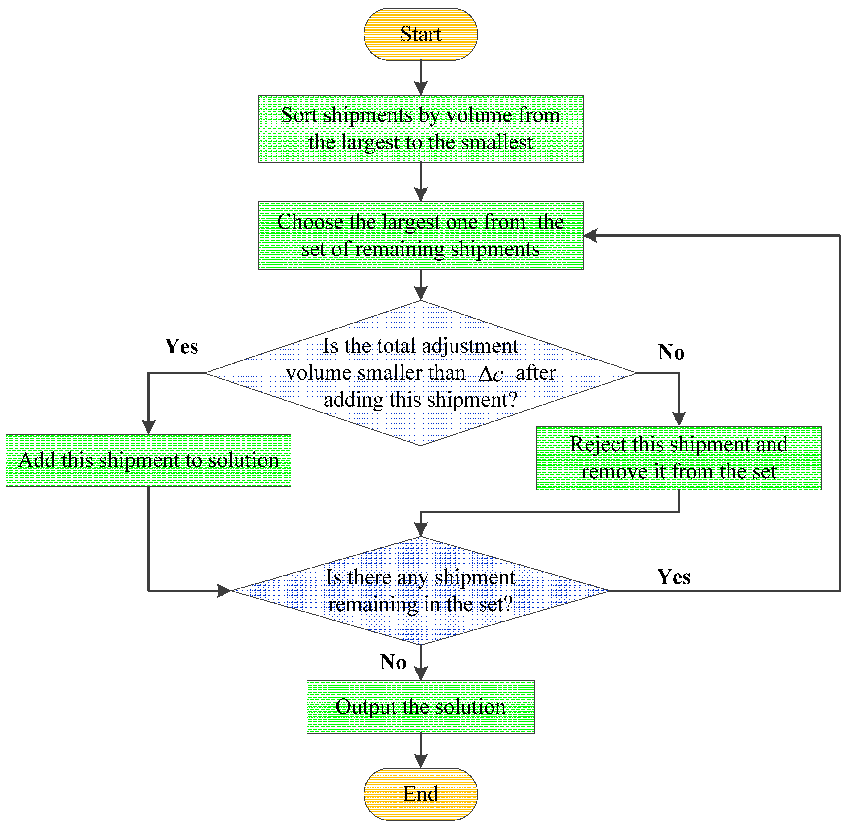
- The greedy choice property.We can make whatever choice seems best at the moment and then solve the sub-problems that arise later. The choice made by a greedy algorithm may depend on the choice made so far, but not on future choices or all the solutions to the sub-problem.
- (2)
- An optimal substructure.A problem exhibits an optimal substructure if an optimal solution to the problem contains optimal solutions to the sub-problem.
4.2.1. Applying the Greedy Algorithm to Model FAP-1 and FAP-2
4.2.2. Applying the Greedy Algorithm to Model FAP-3 and FAP-4
5. Conclusions
Acknowledgments
Author Contributions
Conflicts of Interest
References
- Lin, B.L.; Zhu, S.N.; Chen, Z.S.; Peng, H. The 0-1 integer programming model for optimal car routing problem and algorithm for the available set in rail network. J. Chin. Railw. Soc. 1997, 19, 7–12. [Google Scholar] [CrossRef]
- Du, H.Z.; Ji, L. Study of transportation structure adjustment between lines Jing-Jiu and Jing-Guang. J. Shanghai Jiaotong Univ. 2002, 36, 592–596. [Google Scholar]
- Ye, Y.L.; He, J.; Li, L. Wagon flow organization optimization after building of Xin-Chang railway. J. Tongji Univ. 2003, 31, 1198–1200. [Google Scholar]
- Su, S.H.; Chen, Z.Y. Studies on models and algorithms of optimizing train flow paths in railway network. J. Chin. Railw. Soc. 2008, 30, 29–34. [Google Scholar]
- Tian, Y.M.; Lin, B.L.; Ji, L.J. Railway car flow distribution node-arc and arc-path models based on multi-commodity and virtual arc. J. Chin. Railw. Soc. 2011, 33, 7–12. [Google Scholar]
- Zhao, C.; Yang, L.X.; Li, S.K. Allocating freight empty cars in railway networks with dynamic demands. Discret. Dyn. Nat. Soc. 2014, 2014, 1–12. [Google Scholar] [CrossRef]
- Corman, F.; D’Ariano, A.; Pacciarelli, D.; Pranzo, M. A tabu search algorithm for rerouting trains during rail operations. Transp. Res. B-Meth. 2010, 44, 175–192. [Google Scholar] [CrossRef]
- Sadykov, R.; Lazarev, A.A.; Shiryaev, V.; Stratonnikov, A. Solving a freight railcar flow problem arising in Russia. In Proceedings of the 13th Workshop on Algorithmic Approaches for Transportation Modelling, Optimization, and Systems, Sophia Antipolis, France, 5 September 2013; pp. 55–67. [Google Scholar]
- Borndörfer, R.; Fügenschuh, A.; Klug, T.; Schang, T.; Schlechte, T.; Schülldorf, H. The Freight Train Routing Problem; Angewandte Mathematik und Optimierung Schriftenreihe: Berlin-Dahlem, Germany, 2014. [Google Scholar]
- Zhou, F.; Shi, J.G.; Xu, R.H. Estimation method of path-selecting proportion for urban rail transit based on AFC data. Math. Prob. Eng. 2015, 2015, 1–9. [Google Scholar] [CrossRef]
- Han, B.; Zhou, W.T.; Li, D.W.; Yin, H.D. Dynamic schedule-based assignment model for urban rail transit network with capacity constraints. Sci. World J. 2015, 2015, 1–12. [Google Scholar] [CrossRef] [PubMed]
- Fu, H.L.; Sperry, B.R.; Nie, L. Operational impacts of using restricted passenger flow assignment in high-speed train stop scheduling problem. Math. Prob. Eng. 2013, 2013, 1–8. [Google Scholar] [CrossRef]
- Nguyen, S.; Pallottino, S.; Malucelli, F. A modeling framework for passenger assignment on a transport network with timetables. Transp. Sci. 2001, 35, 238–249. [Google Scholar] [CrossRef]
- Cominetti, R.; Correa, J. Common-lines and passenger assignment in congested transit networks. Transp. Sci. 2001, 35, 250–267. [Google Scholar] [CrossRef]
- Pisinger, D. Where are the hard knapsack problems? Comput. Oper. Res. 2005, 32, 2271–2284. [Google Scholar] [CrossRef]
- Poirriez, V.; Yanev, N.; Andonov, R. A hybrid algorithm for the unbounded knapsack problem. Discret. Optim. 2009, 6, 110–124. [Google Scholar] [CrossRef]
- Frenkel, E.; Nikolaev, A.; Ushakov, A. Knapsack problems in products of groups. J. Symb. Comput. 2016, 74, 96–108. [Google Scholar] [CrossRef]
- Rooderkerk, R.P.; Heerde, H.J. Robust optimization of the 0-1 knapsack problem: Balancing risk and return in assortment optimization. Eur. J. Oper. Res. 2016, 250, 842–854. [Google Scholar] [CrossRef]
- Rao, N.; Shah, P.; Wright, S. Forward-backward greedy algorithms for atomic norm regularization. IEEE Trans. Signal Process. 2015, 63, 5798–5811. [Google Scholar] [CrossRef]
- Davis, S.; Impagliazzo, R. Models of greedy algorithms for graph problems. Algorithmica 2009, 54, 269–317. [Google Scholar] [CrossRef]
- Cerrone, C.; Cerulli, R.; Golden, B. Carousel greedy: A generalized greedy algorithm with applications in optimization. Comput. Oper. Res. 2017, 85, 97–112. [Google Scholar] [CrossRef]

| Parameters | Representation |
|---|---|
| Unit transportation cost. | |
| Length of path A. | |
| Length of path B. | |
| Spare capacity of path A. | |
| Capacity reduction of path A. | |
| Generalized transportation cost. | |
| Unit time cost of shipment . | |
| Unit time cost of shipment . | |
| Average speed of freight trains. | |
| Decision Variables | Representation |
| decision variable. equals 1 if shipment is adjusted to path A; and 0 otherwise. | |
| decision variable. equals 1 if shipment is adjusted to path B; and 0 otherwise. |
| No. | Name | Volume (103 Tons/Year) | (¥/Ton-km) |
|---|---|---|---|
| 1 | 1200 | 0.137 | |
| 2 | 1210 | 0.110 | |
| 3 | 460 | 0.146 | |
| 4 | 1790 | 0.135 | |
| 5 | 650 | 0.108 | |
| 6 | 2310 | 0.115 | |
| 7 | 1540 | 0.126 | |
| 8 | 1760 | 0.112 | |
| 9 | 230 | 0.140 | |
| 10 | 1260 | 0.143 | |
| 11 | 2800 | 0.137 | |
| 12 | 190 | 0.132 | |
| 13 | 200 | 0.125 | |
| 14 | 610 | 0.129 | |
| 15 | 960 | 0.144 | |
| 16 | 1560 | 0.141 | |
| 17 | 720 | 0.107 | |
| 18 | 690 | 0.132 | |
| 19 | 750 | 0.150 | |
| 20 | 370 | 0.114 | |
| 21 | 2250 | 0.129 | |
| 22 | 660 | 0.126 | |
| 23 | 1960 | 0.131 | |
| 24 | 2320 | 0.144 | |
| 25 | 2560 | 0.111 | |
| 26 | 310 | 0.118 | |
| 27 | 2580 | 0.133 | |
| 28 | 110 | 0.146 | |
| 29 | 1360 | 0.118 | |
| 30 | 580 | 0.143 |
| No. | Name | Volume (Tons/Day) | (¥/Ton-km) |
|---|---|---|---|
| 1 | 6113 | 0.103 | |
| 2 | 6677 | 0.158 | |
| 3 | 3812 | 0.107 | |
| 4 | 7697 | 0.110 | |
| 5 | 7572 | 0.153 | |
| 6 | 5607 | 0.126 | |
| 7 | 5279 | 0.100 | |
| 8 | 7341 | 0.109 | |
| 9 | 5749 | 0.111 | |
| 10 | 6256 | 0.123 | |
| 11 | 6245 | 0.145 | |
| 12 | 6874 | 0.114 | |
| 13 | 6494 | 0.130 | |
| 14 | 4028 | 0.115 | |
| 15 | 3782 | 0.109 | |
| 16 | 5519 | 0.148 | |
| 17 | 5491 | 0.120 | |
| 18 | 7970 | 0.152 | |
| 19 | 5874 | 0.104 | |
| 20 | 4437 | 0.132 | |
| 21 | 5482 | 0.130 | |
| 22 | 4292 | 0.146 | |
| 23 | 6771 | 0.125 | |
| 24 | 6028 | 0.154 | |
| 25 | 4870 | 0.138 | |
| 26 | 3592 | 0.128 | |
| 27 | 6471 | 0.143 | |
| 28 | 7617 | 0.135 | |
| 29 | 7868 | 0.150 | |
| 30 | 5135 | 0.122 | |
| 31 | 5047 | 0.121 | |
| 32 | 4611 | 0.123 | |
| 33 | 7562 | 0.104 | |
| 34 | 4567 | 0.152 | |
| 35 | 6223 | 0.116 | |
| 36 | 6287 | 0.118 | |
| 37 | 4722 | 0.145 | |
| 38 | 4253 | 0.126 | |
| 39 | 7688 | 0.130 | |
| 40 | 6153 | 0.100 | |
| 41 | 4723 | 0.146 | |
| 42 | 4047 | 0.119 | |
| 43 | 5801 | 0.119 | |
| 44 | 7909 | 0.134 | |
| 45 | 6931 | 0.125 | |
| 46 | 7898 | 0.146 | |
| 47 | 3817 | 0.159 | |
| 48 | 5958 | 0.124 | |
| 49 | 3593 | 0.148 | |
| 50 | 5096 | 0.106 |
© 2017 by the authors. Licensee MDPI, Basel, Switzerland. This article is an open access article distributed under the terms and conditions of the Creative Commons Attribution (CC BY) license (http://creativecommons.org/licenses/by/4.0/).
Share and Cite
Lin, B.; Liu, S.; Lin, R.; Wu, J.; Wang, J.; Liu, C. Modeling the 0-1 Knapsack Problem in Cargo Flow Adjustment. Symmetry 2017, 9, 118. https://doi.org/10.3390/sym9070118
Lin B, Liu S, Lin R, Wu J, Wang J, Liu C. Modeling the 0-1 Knapsack Problem in Cargo Flow Adjustment. Symmetry. 2017; 9(7):118. https://doi.org/10.3390/sym9070118
Chicago/Turabian StyleLin, Boliang, Siqi Liu, Ruixi Lin, Jianping Wu, Jiaxi Wang, and Chang Liu. 2017. "Modeling the 0-1 Knapsack Problem in Cargo Flow Adjustment" Symmetry 9, no. 7: 118. https://doi.org/10.3390/sym9070118
APA StyleLin, B., Liu, S., Lin, R., Wu, J., Wang, J., & Liu, C. (2017). Modeling the 0-1 Knapsack Problem in Cargo Flow Adjustment. Symmetry, 9(7), 118. https://doi.org/10.3390/sym9070118