The Fuzzy u-Chart for Sustainable Manufacturing in the Vietnam Textile Dyeing Industry

Abstract

The inevitability of measurement errors and/or humans of subjectivity in data collection processes make accumulated data imprecise, and are thus called fuzzy data. To adapt to this fuzzy domain in a manufacturing process, a traditional u control chart for monitoring the average number of nonconformities per unit is required to extend. In this paper, we first generalize the u chart, named fuzzy u-chart, whose control limits are built on the basis of resolution identity, which is a well-known fuzzy set theory. Then, an approach to fuzzy-logic reasoning, incorporating the decision-maker’s varying levels of optimism towards the online process, is proposed to categorize the manufacturing conditions. In addition, we further develop a condition-based classification mechanism, where the process conditions can be discriminated into intermittent states between in-control and out-of-control. As anomalous conditions are monitored to some extent, this condition-based classification mechanism can provide the critical information to deliberate the cost of process intervention with respect to the gain of quality improvement. Finally, the proposed fuzzy u-chart is implemented in the Vietnam textile dyeing industry to replace its conventional u-chart. The results demonstrate that the industry can effectively evade unnecessary adjustments to its current processes; thus, the industry can substantially reduce its operational cost and potential loss.

1. Introduction

Competitive marketplaces require industrial manufacturers to provide consistent and reliable quality products to preserve their survival and sustainable growth. Therefore, the manufacturers keenly explore for optimal strategies to not only lower their percentage of nonconformists, but to also slash manufacturing costs, and to fulfill customer satisfaction [1]. Nowadays, manufacturers pay special efforts in establishing effective quality management systems and programs. Walpole et al. [2] confirmed that the quality-control scheme has been utilized as a powerful tool for manufacturers to achieve their production effectiveness as well as to sustain their quality-based competitive advantages.

Practically, any mistaken intervention of processes, delay of alarming excessive product defects, and scraps or reworks of final products will result in an increase of production costs. Thus, in the monitoring and controlling of online manufacturing processes, Shewhart-type control charts have been widely employed due to their notable capability of early detection of an abnormal process [1,3]. The Shewhart-type control charts fall into two categories, called variable and attribute control charts. While the former monitors the variable-type data, which can be quantitatively measured on a continuous scale such as a thermometer, a weighing scale, or a tape rule, the latter monitors the attribute-type data, which can be qualitatively described, for example, as good or defective, as possessing or not possessing a particular characteristic.

A typical control chart consists of a center line ($CL$) and upper and lower control limits ($UCL$ and $LCL$) for monitoring the process’s key quality characteristic (KQC). Their constructions are based on a moderate number of subgroup KQC samples, where each subgroup sample (randomly drawn) has either an equal or unequal sample size. According to the statistics information of sequentially collected KQC sample data, the control limits categorize the online process condition. When an outlier or any systematic pattern is detected on the chart, it implies the process is affected by some assignable causes where the subsequently well-structured corrective actions are necessitated; otherwise, we conclude that the process is in statistical control, a desired (stable) state where no interference is needed [1].

The establishment of control charts requires fully precise random data gathered from the KQC of the process. However, the natural limitations inherited in practical applications have dampened this possibility. For example, the inevitability of gague errors existing in a measurement system [4,5] and in data collection processes where the human subjectivity arises from the decision-makers’ vast variety of intelligence perceptions and experiences all make accumulated data imprecise [6,7,8,9]. Moreover, for the monitoring and controlling of online manufacturing processes, the traditional control charts carrying a binary classification of the process condition, namely in control and out of control,"have failed to effectively adapt to this fuzzy domain. The extensions of traditional control charts, named “ fuzzy control charts”, become mandated [7,9,10,11,12,13,14].

Over the past decade, worldwide scholars have paid a special interest in proposing and constructing a number of fuzzy control charts; examples include Senturk and Erginel [9] with fuzzy $\tilde{\overline{X}}-\tilde{\overline{R}}$ and $\tilde{\overline{X}}-\tilde{\overline{S}}$ control charts, Shu and Wu [14] with fuzzy $\overline{x}$ and R control charts, Nguyen et al. [15] with fuzzy $\overline{x}$ and s control charts, Shu et al. [4] with fuzzy MaxGWMA control chart, and Morabia et al. [16] with fuzzy $\overline{x}$ control chart to deal with multiple objective decision-making problems. The core issue of the contributions above is centered on the fuzzy-variable control charts.

For the fuzzy-attribute control charts, Wang and Raz [17] pioneered with the linguistic-type KQCs such as perfect, good, medium, poor and bad; unfortunately, Kanagawa et al. [18] claimed that Wang and Raz’s [17] development failed to incorporate the probability distributions for linguistic data when constructing the control charts. Although their assertion is rational in theory, in practice the justifiable probability distributions are not easily determined [19,20]. For other declarations, Shu and Wu [14] and Woodall et al. [21] also emphasized the invalidity of lingistic-type control charts, if their membership functions of linguistic terms were arbitrarily assumed on a given scale without contemplation of induced fuzziness from the judgment of experts.

Moreover, in the fuzzy environment, the binary categorization of the online manufacturing condition still has certain arguments to be fulfilled. Many previous methods performed the binary categorization by defuzzing data on the basis of the fuzzy midrange, fuzzy mode, fuzzy median and fuzzy average; however, such techniques have also raised another consequence of losing the fuzziness information in the manufacturing data where the misclassified possibility of the manufacturing process could be intolerable [14,22,23].

Thus, several approaches to preserve the fuzziness of vague data have been proposed. The evidence can be seen from the necessity index of strict dominance (NISD) by Grzegorzeski and Hryniewicz [24], acceptable percentage index called direct fuzzy approach (DFA) by Gülbay and Kahraman [13], fuzzy dominance approach (FDA) by Shu and Wu [14]. Certain limitations exist in their methods. While the NISD is content-dependent [25], the DFA fails to obtain the fuzzy sample means and variances with the simple using of $\alpha$-cuts [14]. In addition, the FDA approach can only perform nicely at a dominance degree greater than 0.5 [15,26].

To overcome the aforementioned issues, we first generalize the u chart, named fuzzy u-chart whose control limits are built on the basis of Resolution Identity, a well-known fuzzy set theory. Then, an approach of fuzzy-logic reasoning is proposed for the fuzzy control limits to categorize the online manufacturing conditions. Furthermore, we develop a condition-based classification mechanism, where the process conditions can be discriminated into intermittent states between in-control and out-of-control. It can be noted that this novel classification mechanism is rooted on a robust fuzzy-ranking scheme that assesses the magnitude of left-right areas and centroids of fuzzy numbers to provide more satisfactory reasoning [27].

This paper is organized as follows. Section 2 briefly provides key characteristics of the traditional u chart to support part of Section 3, the procedure of constructing the fuzzy u-chart. It is well noted that these two sections depart from the approach presented in [26,28]. Here, the core issue is centered on the fuzzy-attributed control charts, fuzzy u-chart, while Nguyen et al. [26] and Shu et al. [28] stressed on the fuzzy-variable control charts, $\overline{x}$ and s control charts. Section 4 first reviews the Nguyen and Hien’s method [27] which is then extended for better performance of ranking results. We further develop a condition-based classification mechanism, where the process conditions can be discriminated into intermittent states between in-control and out-of-control states. In Section 5, the established fuzzy u-chart is implemented in the Vietnam textile dyeing industry to replace its conventional u-chart. Some concluding remarks make up the last section.

2. Review of Traditional $\mathit{u}$-Chart

Literally, the term “u-chart” is usually used to monitor the average number of nonconformities per unit when the subgroup sample size is either only one inspection unit or several units [1,2]. A nonconformity (also known as a defect) is the product that deviates from a specification, a standard, or an expectation. A nonconforming product usually contains one or more non-conformists whose severity directly influences on the product quality. Typically, the u-chart is constructed as follows:

In m initial samples, let $x_i$ denote the number of non-conformities in the $i^{th}$ sample which has $n_i$ inspection units ($i=\overline{1,m}$). Then, the average number of non-conformists per unit, notated by $u_i$, is calculated by

$$u_i=\frac{x_i}{n_i}$$

(1)

The grand average ${\mu }_u$ of u and variance ${\sigma }^2$ of each sample are defined as

$$\begin{array}{}\mathrm{}& \hfill {\mu }_u& =& \frac{{\sum }_{i=1}^m{x}_i}{{\sum }_{i=1}^m{n}_i}\hfill \mathrm{(2)}& & =& \overline{u}\hfill \mathrm{(3)}& \hfill {\sigma }_{u_i}^2& =& \frac{\overline{u}}{n_i}\hfill \end{array}$$

Therefore, the control limits for u-chart are obtained as

$$\begin{array}{ccc}\hfill UC{L}_u& =& \overline{u}+K\sqrt{\frac{\overline{u}}{n_i}}\hfill \\ \hfill C{L}_u& =& \overline{u}\hfill \\ \hfill LC{L}_u& =& \max \left\{0,\overline{u}-K\sqrt{\frac{\overline{u}}{n_i}}\right\}\hfill \end{array}$$

(4)

where K is the number of standard deviation unit. In common practice, $K=3$ usually used as the scale of an allowable tolerance [1,2].

3. Construction of Fuzzy $\mathit{u}$-Chart

Let us consider m samples each with $n_i(i=\overline{1,m})$ sample size. Let $F{O}_1,F{O}_2,\cdots ,F{O}_m$ be fuzzy observations (fuzzy data) which are assumed to be fuzzy real numbers. Based on those observed fuzzy data, a fuzzy set theory [29,30,31] will be applied to construct the upper and lower control limits for u-chart, which is named fuzzy u-chart.

For any given $\alpha \in [0,1]$ (called $\alpha$ cut), the corresponding real-value data ($\alpha$-level set) $F{O}_{i,\alpha }^L$ and $F{O}_{i,\alpha }^U$ for $i=\overline{1,m}$ are easily acquired. Then the real-value data $F{O}_{1,\alpha }^L,\cdots ,F{O}_{m,\alpha }^L$ and $F{O}_{1,\alpha }^U,\cdots ,F{O}_{m,\alpha }^U$ ($i=\overline{1,m}$) are used in the Equations (1) and (2) for estimating the fuzzy control limits of $F{U}_{i,\alpha }^L$ and $F{U}_{i,\alpha }^U$. The outcome is

$$\begin{array}{ccccccc}\hfill F{U}_{i,\alpha }^U& =& \frac{F{O}_{i,\alpha }^U}{n_i}\hfill & & \hfill F{U}_{i,\alpha }^L& =& \frac{F{O}_{i,\alpha }^L}{n_i}\hfill \\ \hfill {\overline{FU}}_{\alpha }^U& =& \frac{{\sum }_{i=1}^{m}F{O}_{i,\alpha }^U}{{\sum }_{i=1}^m{n}_i}\hfill & & \hfill {\overline{FU}}_{\alpha }^L& =& \frac{{\sum }_{i=1}^{m}F{O}_{i,\alpha }^L}{{\sum }_{i=1}^m{n}_i}\hfill \end{array}$$

Substituting the above parameters into Equation (4), we have the following

$$\left\{\begin{array}{ccccc}u{p}_{F{U}_{i,\alpha }}^U\hfill & \equiv \hfill & {\left(UC{L}_{F{U}_{i,\alpha }}\right)}^U\hfill & =\hfill & {\overline{FU}}_{\alpha }^U+K\sqrt{\frac{{\overline{FU}}_{\alpha }^U}{n_i}}\hfill \\ c_{F{U}_{i,\alpha }}^U\hfill & \equiv \hfill & {\left(C{L}_{F{U}_{i,\alpha }}\right)}^U\hfill & =\hfill & {\overline{FU}}_{\alpha }^U\hfill \\ l{o}_{F{U}_{i,\alpha }}^U\hfill & \equiv \hfill & {\left(LC{L}_{F{U}_{i,\alpha }}\right)}^U\hfill & =\hfill & max\left\{0,{\overline{FU}}_{\alpha }^U-K\sqrt{\frac{{\overline{FU}}_{\alpha }^U}{n_i}}\right\}\hfill \end{array}\right.$$

$$\left\{\begin{array}{ccccc}u{p}_{F{U}_{i,\alpha }}^L\hfill & \equiv \hfill & {\left(UC{L}_{F{U}_{i,\alpha }}\right)}^L\hfill & =\hfill & {\overline{FU}}_{\alpha }^L+K\sqrt{\frac{{\overline{FU}}_{\alpha }^L}{n_i}}\hfill \\ c_{F{U}_{i,\alpha }}^L\hfill & \equiv \hfill & {\left(C{L}_{F{U}_{i,\alpha }}\right)}^L\hfill & =\hfill & {\overline{FU}}_{\alpha }^L\hfill \\ l{o}_{F{U}_{i,\alpha }}^L\hfill & \equiv \hfill & {\left(LC{L}_{F{U}_{i,\alpha }}\right)}^L\hfill & =\hfill & max\left\{0,{\overline{FU}}_{\alpha }^L-K\sqrt{\frac{{\overline{FU}}_{\alpha }^L}{n_i}}\right\}\hfill \end{array}\right.$$

(a)  Construction of Fuzzy Upper Control Limit ${\widetilde{up}}_{F{U}_i}$

Let’s consider the closed interval $A_{i,\alpha }$ according to the results above. We define

$$A_{i,\alpha }=\left[min\left\{u{p}_{F{U}_{i,\alpha }}^L,u{p}_{F{U}_{i,\alpha }}^U\right\},max\left\{u{p}_{F{U}_{i,\alpha }}^L,u{p}_{F{U}_{i,\alpha }}^U\right\}\right]\equiv \left[l{u}_{i,\alpha },u{u}_{i,\alpha }\right]$$

where

$$l{u}_{i,\alpha }=min\left\{u{p}_{F{U}_{i,\alpha }}^L,u{p}_{F{U}_{i,\alpha }}^U\right\}$$

(5)

$$u{u}_{i,\alpha }=max\left\{u{p}_{F{U}_{i,\alpha }}^L,u{p}_{F{U}_{i,\alpha }}^U\right\}$$

(6)

By applying the resolution-identity theorem [29,30,31], the membership function of the upper control limit, one of the control limits’ fuzzy numbers (CLFNs) can be defined as

$${\xi }_{{\widetilde{up}}_{F{U}_i}}\left(c\right)=\underset{\alpha \in [0,1]}{sup}\alpha ·1_{A_{i,\alpha }}\left(c\right).$$

Since each $F{O}_i$ is a fuzzy real number, $F{U}_{i,\alpha }^L$ and $F{U}_{i,\alpha }^U$ are continuous with respect to $\alpha$ on [0, 1]. As a consequence, the $\alpha$-level set ${\widetilde{up}}_{F{U}_{i,\alpha }}$ of fuzzy upper control limit ${\widetilde{up}}_{F{U}_i}$ can be simply rewritten as

$$\begin{array}{ccc}\hfill {\widetilde{up}}_{F{U}_{i,\alpha }}& =& \left\{c:{\xi }_{F{U}_i}\left(c\right)\ge \alpha \right\}\hfill \\ & =& \left[\underset{\alpha \le \beta \le 1}{min}l{u}_{i,\beta },\underset{\alpha \le \beta \le 1}{max}u{u}_{i,\beta }\right]\hfill \\ & =& \left[{\left({\widetilde{up}}_{F{U}_i}\right)}_{\alpha }^L,{\left({\widetilde{up}}_{F{U}_i}\right)}_{\alpha }^U\right]\hfill \end{array}$$

(7)

where $l{u}_{i,\alpha }$ and $u{u}_{i,\alpha }$ are shown in Equations (5) and (6).

Furthermore, from Equation (7), the relationship between ${\left({\widetilde{up}}_{F{U}_i}\right)}_{\alpha }^L$ and $u{p}_{F{U}_{i,\alpha }}^L,u{p}_{F{U}_{i,\alpha }}^U$ is found as

$$\begin{array}{ccc}\hfill {\left({\widetilde{up}}_{F{U}_i}\right)}_{\alpha }^L& =& \underset{\alpha \le \beta \le 1}{min}l{u}_{i,\beta }\hfill \\ & =& \underset{\alpha \le \beta \le 1}{min}min\left\{u{p}_{F{U}_{i,\beta }}^L,u{p}_{F{U}_{i,\beta }}^U\right\}.\hfill \end{array}$$

(8)

Similarly, the relationship between ${\left({\widetilde{up}}_{F{U}_i}\right)}_{\alpha }^U$ and $u{p}_{F{U}_{i,\alpha }}^L,u{p}_{F{U}_{i,\alpha }}^U$ is

$$\begin{array}{ccc}\hfill {\left({\widetilde{up}}_{F{U}_i}\right)}_{\alpha }^U& =& \underset{\alpha \le \beta \le 1}{max}u{u}_{i,\beta }\hfill \\ & =& \underset{\alpha \le \beta \le 1}{max}max\left\{u{p}_{F{U}_{i,\beta }}^L,u{p}_{F{U}_{i,\beta }}^U\right\}.\hfill \end{array}$$

(9)

(b)  Construction of Fuzzy Lower Control Limit $F{L}_{F{U}_i}$

Likewise, let us consider the closed interval $B_{i,\alpha }$. We define

$$B_{i,\alpha }=\left[min\left\{l{o}_{F{U}_{i,\alpha }}^L,l{o}_{F{U}_{i,\alpha }}^U\right\},max\left\{l{o}_{F{U}_{i,\alpha }}^L,l{o}_{F{U}_{i,\alpha }}^U\right\}\right]\equiv \left[l{l}_{i,\alpha },u{l}_{i,\alpha }\right]$$

where

$$l{l}_{i,\alpha }=min\left\{l{o}_{F{U}_{i,\alpha }}^L,l{o}_{F{U}_{i,\alpha }}^U\right\}$$

(10)

$$u{l}_{i,\alpha }=max\left\{l{o}_{F{U}_{i,\alpha }}^L,l{o}_{F{U}_{i,\alpha }}^U\right\}$$

(11)

From the resolution-identity theorem [29,30,31], the membership function of the lower control limit, one of CLFNs is determined by

$${\xi }_{{\widetilde{lo}}_{F{U}_i}}\left(c\right)=\underset{\alpha \in [0,1]}{sup}\alpha ·1_{B_{I,\alpha }}\left(c\right).$$

Since each $F{O}_i$ is a fuzzy real number, $F{U}_{i,\alpha }^L$ and $F{U}_{i,\alpha }^U$ are continuous over $\alpha$ on [0, 1]. Hence, the $\alpha$-level set ${\widetilde{lo}}_{F{U}_{i,\alpha }}$ of fuzzy upper control limit ${\widetilde{lo}}_{F{U}_i}$ can be simply attained as

$$\begin{array}{ccc}\hfill {\widetilde{lo}}_{F{U}_{i,\alpha }}& =& \left\{c:{\xi }_{F{U}_i}\left(c\right)\ge \alpha \right\}\hfill \\ & =& \left[\underset{\alpha \le \beta \le 1}{min}l{l}_{i,\beta },\underset{\alpha \le \beta \le 1}{max}u{l}_{i,\beta }\right]\hfill \\ & =& \left[{\left({\widetilde{lo}}_{F{U}_i}\right)}_{\alpha }^L,{\left({\widetilde{lo}}_{F{U}_i}\right)}_{\alpha }^U\right]\hfill \end{array}$$

(12)

where $l{l}_{i,\alpha }$ and $u{l}_{i,\alpha }$ are expressed in Equations (10) and (11).

From Equation (12), the corresponding between ${\left({\widetilde{lo}}_{F{U}_i}\right)}_{\alpha }^L$ and $l{o}_{F{U}_{i,\alpha }}^L,l{o}_{F{U}_{i,\alpha }}^U$ is realized as

$$\begin{array}{ccc}\hfill {\left({\widetilde{lo}}_{F{U}_i}\right)}_{\alpha }^L& =& \underset{\alpha \le \beta \le 1}{min}l{l}_{i,\beta }\hfill \\ & =& \underset{\alpha \le \beta \le 1}{min}min\left\{l{o}_{F{U}_{i,\beta }}^L,l{o}_{F{U}_{i,\beta }}^U\right\}.\hfill \end{array}$$

(13)

Likewise, the relation between ${\left({\widetilde{lo}}_{F{U}_i}\right)}_{\alpha }^U$ and $l{o}_{F{U}_{i,\alpha }}^L,l{o}_{F{U}_{i,\alpha }}^U$ is

$$\begin{array}{ccc}\hfill {\left({\widetilde{lo}}_{F{U}_i}\right)}_{\alpha }^U& =& \underset{\alpha \le \beta \le 1}{max}u{l}_{i,\beta }\hfill \\ & =& \underset{\alpha \le \beta \le 1}{max}max\left\{l{o}_{F{U}_{i,\beta }}^L,l{o}_{F{U}_{i,\beta }}^U\right\}.\hfill \end{array}$$

(14)

4. Classification Conditions

In this section, we will first review a fuzzy ranking method proposed by Nguyen and Hien [27], and then extend their ranking rules to provide more satisfactory reasoning for classifying manufacturing process conditions. Its preferable performance over the previous study in certain cases is illustrated by the comparative analysis shown in Section 5.

4.1. Ranking Fuzzy Numbers with Nguyen & Hien’s Approach

Let’s consider n fuzzy numbers $A_i=(a_i,b_i,c_i,d_i;w_i)(i=\overline{1,n})$. The membership functions of the i th number are defined as

$${\xi }_{A_i}\left(x\right)=\left\{\begin{array}{cc}{f}_{A_i}^L\left(x\right)\hfill & \mathrm{if}x\in [b_i,c_i]\hfill \\ w_i\hfill & \mathrm{if}x\in [c_i,d_i]\hfill \\ f_{A_i}^R\left(x\right)\hfill & \mathrm{if}x\in [d_i,e_i]\hfill \\ 0\hfill & \mathrm{otherwise},\hfill \end{array}\right.$$

Let $g_{A_i}^L\left(y\right)$ and $g_{A_i}^R\left(y\right)$ respectively denote the inverse functions of ${\xi }_{A_i}^L\left(x\right)$ and ${\xi }_{A_i}^R\left(x\right)$. We also define $a_{min}=min\{a_1,\cdots ,a_n\}$ and $d_{max}=max\{d_1,\cdots ,d_n\}$.

Definition 1.

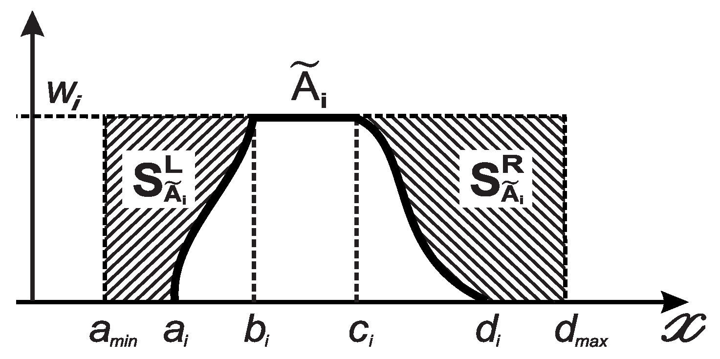
(Left-Right areas) The left area of $A_i$, $S_{A_i}^L$, which is from the $a_{min}$ to $g_{A_i}^L\left(y\right)$, can be defined as

$$S_{A_i}^L={\int }_0^{w_i}\left[g_{A_i}^L\left(y\right)-a_{min}\right]dy.$$

(15)

and its right area, $S_{A_i}^R$, which goes from $g_{A_i}^R\left(y\right)$ to $d_{max}$, can be set as

$$S_{A_i}^R={\int }_0^{w_i}\left[d_{max}-g_{A_i}^R\left(y\right)\right]dy.$$

(16)

The $S_{A_i}^L$ and $S_{A_i}^R$ are visually plotted on Figure 1 [32,33,34,35,36].

Definition 2.

An expectation value of centroid of $A_i$, denoted by $E{C}_i$, is defined [32,33,37,38,39,40] as

$$E{C}_i=\frac{{\int }_{a_i}^{d_i}x{\xi }_{A_i}\left(x\right)dx}{{\int }_{a_i}^{d_i}{\xi }_{A_i}\left(x\right)dx}.$$

(17)

From the statistical point of view, $E{C}_i$ is the weighted mean of $A_i$. It implies that when $A_i=(a,a,a,a;w_i)$, we can have $C{V}_i=a$.

From the above definitions, Nguyen and Hien [27] proposed a ranking index for $A_i=(a_i,b_i,c_i,d_i;w_i)$ $(i=\overline{1,n})$ at each level of $\beta$, denoted by $LRA{C}_i^{\beta }$.

$$LRA{C}_i^{\beta }=\left[\beta S_{A_i}^R+(1-\beta )S_{A_i}^L\right]E{C}_i$$

(18)

where $\beta \in [0,1]$ is called “level of optimism” that presents the decision-maker’s attitude towards risk. The $\beta =0$ indicates “the decision-maker with a totally pessimistic attitude towards risk”, $\beta =1$ indicates “the decision-maker with a totally optimistic attitude towards risk”, and $\beta =0.5$ indicates “the decision-maker with a neutral attitude towards risk”.

Two fuzzy numbers $A_i$ and $A_j$ can be ranked by applying the following rules:

• $A_i\succ A_j$ at the optimism level of $\beta$ if and only if $LRA{C}_i^{\beta }>LRA{C}_j^{\beta }$.
• $A_i\prec A_j$ at the optimism level of $\beta$ if and only if $LRA{C}_i^{\beta }<LRA{C}_j^{\beta }$.
• $A_i\approx A_j$ at the optimism level of $\beta$ if and only if $LRA{C}_i^{\beta }=LRA{C}_j^{\beta }$.

Notably, Nguyen and Hien [27] showed that the expectation value of the centroid $E{C}_i$ for the $LRAC$ index magnifies the ranking discriminatory power; hence, the method has more efficient results in many cases than that of Yu & Dat [34].

4.2. Our Extended Ranking Rules

Now, let’s consider $D{S}_{i-j}^{\beta }$, the disparity amount of $A_i$’s and $A_j$’s ranking indexes at the optimism level of $\beta$.

$$\begin{array}{ccc}\hfill D{S}_{i-j}^{\beta }& =& LRA{C}_i^{\beta }-LRA{C}_j^{\beta }\hfill \\ & =& \beta \left(S_{A_i}^{R}E{C}_i-S_{A_j}^{R}E{C}_j\right)+(1-\beta )\left(S_{A_i}^{L}E{C}_i-S_{A_j}^{L}E{C}_j\right)\hfill \\ \hfill D{S}_{i-j}^{\beta }& =& \beta ▵SE{C}_{i-j}^R+(1-\beta )▵SE{C}_{i-j}^L\hfill \end{array}$$

(19)

where $▵SE{C}_{i-j}^R=S_{A_i}^{R}E{C}_i-S_{A_j}^{R}E{C}_j$ and $▵SE{C}_{i-j}^L=S_{A_i}^{L}E{C}_i-S_{A_j}^{L}E{C}_j$.

With Equation (19), the ranking rules mentioned in Section 4.1 can be rewritten as

• $A_i\succ A_j$ at the optimism level of $\beta$ if and only if $D{S}_{i-j}^{\beta }>0$.
• $A_i\prec A_j$ at the optimism level of $\beta$ if and only if $D{S}_{i-j}^{\beta }<0$.
• $A_i\approx A_j$ at the optimism level of $\beta$ if and only if $D{S}_{i-j}^{\beta }=0$.

Because $D{S}_{i-j}^{\beta }$, expressed in Equation (19), is a monotonous function of $\beta$, then $D{S}_{i-j}^{\beta }=0$ can only occur in the following two cases

• $▵SE{C}_{i-j}^R<0$ and $▵SE{C}_{i-j}^L>0$; or,
• $▵SE{C}_{i-j}^R>0$ and $▵SE{C}_{i-j}^L<0$.

Furthermore, to sufficiently represent the fuzziness information residing in the collected data, we propose an alternative approach. This approach is capable of comparing two fuzzy numbers into four linguistic-sense consequences that include larger “≻”, rather larger “⪰”, rather smaller “⪯”, and smaller “≺”.

To achieve this, we first define three new terms, namely “benchmark level ${\beta }_0$”, “step of change in the optimism level $▵\beta$” and “unit ranking”.

Definition 3.

The benchmark level ${\beta }_0\in (0,1)$ is an optimism level at which $D{S}_{i-j}^{{\beta }_0}$ is equal to 0.

Definition 4.

The step of change in the optimism level ($▵\beta$) is the fixed difference between two consecutive optimism levels. The $▵\beta ={\beta }_{i+1}-{\beta }_i$ is a constant for the n optimism levels ${\beta }_1,{\beta }_2,\cdots ,{\beta }_n$.

Definition 5.

The unit disparity is the disparity of ranking indexes of $A_i$ and $A_j$ caused by the step of change of the optimism level.

In addition, in consideration of the difference of $D{S}_{i-j}^{\beta }$ at $▵\beta$, the Definition 5 can be further derived as

$$\begin{array}{ccc}\hfill ▵D{S}_{i-j}^{{\beta }_2-{\beta }_1}& =& |D{S}_{i-j}^{{\beta }_2}-D{S}_{i-j}^{{\beta }_1}|\hfill \\ & =& ({\beta }_2-{\beta }_1)|▵SE{C}_{i-j}^R-▵SE{C}_{i-j}^L|\hfill \\ \hfill ▵D{S}_{i-j}^{▵\beta }& =& ▵\beta |▵SE{C}_{i-j}^R-▵SE{C}_{i-j}^L|\hfill \end{array}$$

(20)

Here $▵D{S}_{i-j}^{▵\beta }$ represents a change difference of the disparity obtained from $A_i$’s and $A_j$’s ranking indexes. For a given $▵\beta$, the $▵D{S}_{i-j}^{▵\beta }$ can be easily acquired.

Therefore, two arbitrarily chosen fuzzy numbers $A_i$ and $A_j$ can be ranked according to the following rules

(1)

$A_1\succ A_2$ if and only if one of the conditions below occurs

$$\left[\begin{array}{c}D{S}_{i-j}^{\beta }>0\forall \beta \in [0,1];\hfill \\ \left(D{S}_{i-j}^{\beta }-D{S}_{i-j}^{{\beta }_0}\right)>▵D{S}_{i-j}^{▵\beta }>0.\hfill \end{array}\right.$$

(2)

$A_i\prec A_j$ if and only if one of the below conditions holds

$$\left[\begin{array}{c}D{S}_{i-j}^{\beta }<0\forall \beta \in [0,1];\hfill \\ \left(D{S}_{i-j}^{\beta }-D{S}_{i-j}^{{\beta }_0}\right)<-▵D{S}_{i-j}^{▵\beta }<0.\hfill \end{array}\right.$$

(3)

$A_i⪰A_j$ at the optimism level $\beta$ if and only if

$$\left\{\begin{array}{c}▵SE{C}_{i-j}^R\times ▵SE{C}_{i-j}^L<0\hfill \\ 0<D{S}_{i-j}^{\beta }\le ▵D{S}_{i-j}^{▵\beta }\hfill \end{array}\right.$$

(4)

$A_i⪯A_j$ at the optimism level $\beta$ if and only if

$$\left\{\begin{array}{c}▵SE{C}_{i-j}^R\times ▵SE{C}_{i-j}^L<0\hfill \\ -▵D{S}_{i-j}^{▵\beta }\le D{S}_{i-j}^{\beta }\le 0.\hfill \end{array}\right.$$

4.3. Proposed Classification

By integrating the aforementioned fuzzy u-chart and fuzzy ranking approach, we are able to categorize the online manufacturing conditions.

Based on $F{U}_i$, a fuzzy average number obtained from Section 3, we further develop condition-based classification rules with respect to a certain optimism level $\beta$, where the process conditions can be discriminated into intermittent states between in-control and out-of-control.

(1)

The process is in-control if one of the below situations holds

$\left(a\right)\left\{\begin{array}{ccc}D{S}_{{\widetilde{up}}_{F{U}_i}-F{U}_i}^{\beta }\hfill & >\hfill & 0\forall \beta \in [0,1]\hfill \\ D{S}_{F{U}_i-{\widetilde{lo}}_{F{U}_i}}^{\beta }\hfill & >\hfill & 0\forall \beta \in [0,1]\hfill \end{array}\right.$

$\left(b\right)\left\{\begin{array}{ccc}D{S}_{{\widetilde{up}}_{F{U}_i}-F{U}_i}^{\beta }\hfill & >\hfill & ▵D{S}_{{\widetilde{up}}_{F{U}_i}-F{U}_i}^{▵\beta }\hfill \\ ▵SE{C}_{{\widetilde{up}}_{F{U}_i}-F{U}_i}^L\times ▵SE{C}_{{\widetilde{up}}_{F{U}_i}-F{U}_i}^R\hfill & <\hfill & 0\hfill \\ D{S}_{F{U}_i-{\widetilde{lo}}_{F{U}_i}}^{\beta }\hfill & >\hfill & ▵D{S}_{F{U}_i-{\widetilde{lo}}_{F{U}_i}}^{▵\beta }\hfill \\ ▵SE{C}_{F{U}_i-{\widetilde{lo}}_{F{U}_i}}^L\times ▵SE{C}_{F{U}_i-{\widetilde{lo}}_{F{U}_i}}^R\hfill & <\hfill & 0\hfill \end{array}\right.$

$\left(c\right)\left\{\begin{array}{ccc}D{S}_{{\widetilde{up}}_{F{U}_i}-F{U}_i}^{\beta }\hfill & >\hfill & 0\forall \beta \in [0,1]\hfill \\ D{S}_{F{U}_i-{\widetilde{lo}}_{F{U}_i}}^{\beta }\hfill & >\hfill & ▵D{S}_{F{U}_i-{\widetilde{lo}}_{F{U}_i}}^{▵\beta }\hfill \\ ▵SE{C}_{F{U}_i-{\widetilde{lo}}_{F{U}_i}}^L\times ▵SE{C}_{F{U}_i-{\widetilde{lo}}_{F{U}_i}}^R\hfill & <\hfill & 0\hfill \end{array}\right.$

$\left(d\right)\left\{\begin{array}{ccc}D{S}_{F{U}_i-{\widetilde{lo}}_{F{U}_i}}^{\beta }\hfill & >\hfill & 0\forall \beta \in [0,1]\hfill \\ D{S}_{{\widetilde{up}}_{F{U}_i}-F{U}_i}^{\beta }\hfill & >\hfill & ▵D{S}_{{\widetilde{up}}_{F{U}_i}-F{U}_i}^{▵\beta }\hfill \\ ▵SE{C}_{{\widetilde{up}}_{F{U}_i}-F{U}_i}^L\times ▵SE{C}_{{\widetilde{up}}_{F{U}_i}-F{U}_i}^R\hfill & <\hfill & 0\hfill \end{array}\right.$

(2)

The process is out of control if one of the following conditions is true

$\left(a\right)\begin{array}{c}D{S}_{{\widetilde{up}}_{F{U}_i}-F{U}_i}^{\beta }<0\forall \beta \in [0,1].\hfill \end{array}$

$\left(b\right)\left\{\begin{array}{ccc}D{S}_{{\widetilde{up}}_{F{U}_i}-F{U}_i}^{\beta }\hfill & >\hfill & 0\forall \beta \in [0,1]\hfill \\ D{S}_{F{U}_i-{\widetilde{lo}}_{F{U}_i}}^{\beta }\hfill & \le \hfill & -▵D{S}_{F{U}_i-{\widetilde{lo}}_{F{U}_i}}^{▵\beta }\hfill \\ ▵SE{C}_{F{U}_i-{\widetilde{lo}}_{F{U}_i}}^L\times ▵SE{C}_{F{U}_i-{\widetilde{lo}}_{F{U}_i}}^R\hfill & <\hfill & 0\hfill \end{array}\right.$

$\left(c\right)\begin{array}{c}D{S}_{F{U}_i-{\widetilde{lo}}_{F{U}_i}}^{\beta }<0\forall \beta \in [0,1].\hfill \end{array}$

$\left(d\right)\left\{\begin{array}{ccc}D{S}_{F{U}_i-{\widetilde{lo}}_{F{U}_i}}^{\beta }\hfill & >\hfill & 0\forall \beta \in [0,1]\hfill \\ D{S}_{{\widetilde{up}}_{F{U}_i}-F{U}_i}^{\beta }\hfill & \le \hfill & -▵D{S}_{{\widetilde{up}}_{F{U}_i}-F{U}_i}^{▵\beta }\hfill \\ ▵SE{C}_{{\widetilde{up}}_{F{U}_i}-F{U}_i}^L\times ▵SE{C}_{{\widetilde{up}}_{F{U}_i}-F{U}_i}^R\hfill & <\hfill & 0\hfill \end{array}\right.$

(3)

The process is rather in-control if one of the below situations occurs

$\left(a\right)\left\{\begin{array}{ccc}D{S}_{{\widetilde{up}}_{F{U}_i}-F{U}_i}^{\beta }\hfill & >\hfill & 0\forall \beta \in [0,1]\hfill \\ D{S}_{F{U}_i-{\widetilde{lo}}_{F{U}_i}}^{\beta }\hfill & \le \hfill & ▵D{S}_{F{U}_i-{\widetilde{lo}}_{F{U}_i}}^{▵\beta }\hfill \\ D{S}_{F{U}_i-{\widetilde{lo}}_{F{U}_i}}^{\beta }\hfill & >\hfill & 0\hfill \\ ▵SE{C}_{F{U}_i-{\widetilde{lo}}_{F{U}_i}}^L\times ▵SE{C}_{F{U}_i-{\widetilde{lo}}_{F{U}_i}}^R\hfill & <\hfill & 0\hfill \end{array}\right.$

$\left(b\right)\left\{\begin{array}{ccc}D{S}_{F{U}_i-{\widetilde{lo}}_{F{U}_i}}^{\beta }\hfill & >\hfill & 0\forall \beta \in [0,1]\hfill \\ D{S}_{{\widetilde{up}}_{F{U}_i}-F{U}_i}^{\beta }\hfill & \le \hfill & ▵D{S}_{{\widetilde{up}}_{F{U}_i}-F{U}_i}^{▵\beta }\hfill \\ D{S}_{{\widetilde{up}}_{F{U}_i}-F{U}_i}^{\beta }\hfill & >\hfill & 0\hfill \\ ▵SE{C}_{{\widetilde{up}}_{F{U}_i}-F{U}_i}^L\times ▵SE{C}_{{\widetilde{up}}_{F{U}_i}-F{U}_i}^R\hfill & <\hfill & 0\hfill \end{array}\right.$

$\left(c\right)\left\{\begin{array}{ccc}D{S}_{{\widetilde{up}}_{F{U}_i}-F{U}_i}^{\beta }\hfill & \le \hfill & ▵D{S}_{{\widetilde{up}}_{F{U}_i}-F{U}_i}^{▵\beta }\hfill \\ D{S}_{{\widetilde{up}}_{F{U}_i}-F{U}_i}^{\beta }\hfill & >\hfill & 0\hfill \\ ▵SE{C}_{{\widetilde{up}}_{F{U}_i}-F{U}_i}^L\times ▵SE{C}_{{\widetilde{up}}_{F{U}_i}-F{U}_i}^R\hfill & <\hfill & 0\hfill \\ D{S}_{F{U}_i-{\widetilde{lo}}_{F{U}_i}}^{\beta }\hfill & \le \hfill & ▵D{S}_{F{U}_i-{\widetilde{lo}}_{F{U}_i}}^{▵\beta }\hfill \\ D{S}_{F{U}_i-{\widetilde{lo}}_{F{U}_i}}^{\beta }\hfill & >\hfill & 0\hfill \\ ▵SE{C}_{F{U}_i-{\widetilde{lo}}_{F{U}_i}}^L\times ▵SE{C}_{F{U}_i-{\widetilde{lo}}_{F{U}_i}}^R\hfill & <\hfill & 0\hfill \end{array}\right.$

(4)

The process is rather out-of-control if one of the following conditions is fulfilled

$\left(a\right)\left\{\begin{array}{ccc}D{S}_{{\widetilde{up}}_{F{U}_i}-F{U}_i}^{\beta }\hfill & >\hfill & 0\forall \beta \in [0,1]\hfill \\ D{S}_{F{U}_i-{\widetilde{lo}}_{F{U}_i}}^{\beta }\hfill & >\hfill & -▵D{S}_{F{U}_i-{\widetilde{lo}}_{F{U}_i}}^{▵\beta }\hfill \\ D{S}_{F{U}_i-{\widetilde{lo}}_{F{U}_i}}^{\beta }\hfill & \le \hfill & 0\hfill \\ ▵SE{C}_{F{U}_i-{\widetilde{lo}}_{F{U}_i}}^L\times ▵SE{C}_{F{U}_i-{\widetilde{lo}}_{F{U}_i}}^R\hfill & <\hfill & 0\hfill \end{array}\right.$

$\left(b\right)\left\{\begin{array}{ccc}D{S}_{{\widetilde{up}}_{F{U}_i}-F{U}_i}^{\beta }\hfill & >\hfill & 0\hfill \\ ▵SE{C}_{{\widetilde{up}}_{F{U}_i}-F{U}_i}^L\times ▵SE{C}_{{\widetilde{up}}_{F{U}_i}-F{U}_i}^R\hfill & <\hfill & 0\hfill \\ D{S}_{F{U}_i-{\widetilde{lo}}_{F{U}_i}}^{\beta }\hfill & >\hfill & -▵D{S}_{F{U}_i-{\widetilde{lo}}_{F{U}_i}}^{▵\beta }\hfill \\ D{S}_{F{U}_i-{\widetilde{lo}}_{F{U}_i}}^{\beta }\hfill & \le \hfill & 0\hfill \\ ▵SE{C}_{F{U}_i-{\widetilde{lo}}_{F{U}_i}}^L\times ▵SE{C}_{F{U}_i-{\widetilde{lo}}_{F{U}_i}}^R\hfill & <\hfill & 0\hfill \end{array}\right.$

$\left(c\right)\left\{\begin{array}{ccc}D{S}_{F{U}_i-{\widetilde{lo}}_{F{U}_i}}^{\beta }\hfill & >\hfill & 0\forall \beta \in [0,1]\hfill \\ D{S}_{{\widetilde{up}}_{F{U}_i}-F{U}_i}^{\beta }\hfill & >\hfill & -▵D{S}_{{\widetilde{up}}_{F{U}_i}-F{U}_i}^{▵\beta }\hfill \\ D{S}_{{\widetilde{up}}_{F{U}_i}-F{U}_i}^{\beta }\hfill & \le \hfill & 0\hfill \\ ▵SE{C}_{{\widetilde{up}}_{F{U}_i}-F{U}_i}^L\times ▵SE{C}_{{\widetilde{up}}_{F{U}_i}-F{U}_i}^R\hfill & <\hfill & 0\hfill \end{array}\right.$

$\left(d\right)\left\{\begin{array}{ccc}D{S}_{F{U}_i-{\widetilde{lo}}_{F{U}_i}}^{\beta }\hfill & >\hfill & 0\hfill \\ ▵SE{C}_{F{U}_i-{\widetilde{lo}}_{F{U}_i}}^L\times ▵SE{C}_{F{U}_i-{\widetilde{lo}}_{F{U}_i}}^R\hfill & <\hfill & 0\hfill \\ D{S}_{{\widetilde{up}}_{F{U}_i}-F{U}_i}^{\beta }\hfill & >\hfill & -▵D{S}_{{\widetilde{up}}_{F{U}_i}-F{U}_i}^{▵\beta }\hfill \\ D{S}_{{\widetilde{up}}_{F{U}_i}-F{U}_i}^{\beta }\hfill & \le \hfill & 0\hfill \\ ▵SE{C}_{{\widetilde{up}}_{F{U}_i}-F{U}_i}^L\times ▵SE{C}_{{\widetilde{up}}_{F{U}_i}-F{U}_i}^R\hfill & <\hfill & 0\hfill \end{array}\right.$

Remark 1.

The procedure to conduct our fuzzy u-chart and evaluate the process performance is briefly generalized as follows:

Step 1:

From the collected data, we first construct the fuzzy control limits as presented in Section 3.

Step 2:

With each ${\widetilde{up}}_{F{U}_i}$, ${\widetilde{lo}}_{F{U}_i}$, and $F{U}_i$, calculate its left area, right area and expected centroid as shown in Definition 1 and 2.

Step 3:

For each β, calculate $D{S}^{\beta }$, $▵SE{C}^L$, and $▵SE{C}^R$ for each pair (${\widetilde{up}}_{F{U}_i}$, $F{U}_i$) and ($F{U}_i$, ${\widetilde{lo}}_{F{U}_i}$) from Equation (19).

Step 4:

With a given $▵\beta$, calculate $▵D{S}^{▵\beta }$ for each pair (${\widetilde{up}}_{F{U}_i}$, $F{U}_i$) and ($F{U}_i$, ${\widetilde{lo}}_{F{U}_i}$) from Equation (20).

Step 5:

The results obtained from Step 3 and 4 are used in the classification mechanism presented in Section 4.3.

5. Practical Application

The recent advances in science, technology, and global integration have led to profound competition amongst businesses. As customers nowadays have a stronger negotiating power, providing them better quality products/services with a reasonable price becomes ever so critical to the survival and development of every business organization [41,42]. Lee et al. [43] indicated that a failure in achieving customers’ expected quality will lead to a long production cycle time, an increase in production and warranty cost, as well as a significant defection in the number of customers.

In practice, there are several controllable and uncontrollable factors affecting the quality of industrial products. In several labor-intensive industries, for example, textile/garment and footwear industries, workmanship is identified as one of the key factors. The importance of workmanship is derived from major parts of the processes being handled by workers practical working experience, which directly influences the quality of the products manufactured. In such industries, the quality of final products practically depends on the subjective perception, knowledge, mood and behavior of the inspectors, also known as quality controllers or assurers who check individual parts, semi-products and final products at different stages in the processes to make sure that their products meet certain specifications set by customers [41]. Consequently, with the manual inspection of random samples, certain limitations in terms of inaccuracy, inconsistency and inefficiency, are obviously inevitable; hence, the recorded data are considered fuzzy [4,41,44]. To have more objective evaluation, automatic inspection systems have been preferably installed despite of their high cost [42].

Literally, Wong et al. [41] provided a critical review of several approaches in detecting different defects and found that their focus was mainly on defect detection instead of defect diagnosis to identify root causes of defects and implement corrective actions. Lee et al. [43] further pinpointed that the existing detection methods treat defects individually without considering their relationships. As a consequence, the general performance of manufacturing processes fails to be appropriately monitored to implement proper adjustments to improve the product quality. To fulfill the gap in the fuzzy environment, this paper proposes using the fuzzy u-chart with the classification mechanism discussed in Section 4.3. To evaluate the performance of our proposed fuzzy u-chart, we employed the chart in a typical example of monitoring the defects in dyed cloth in textile industry.

5.1. Construction of Fuzzy u-Chart

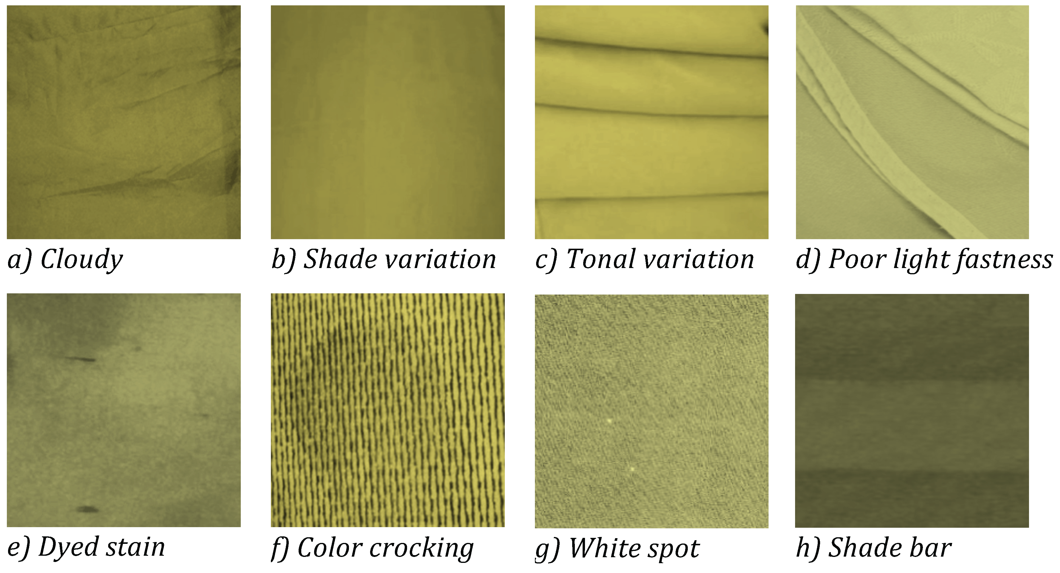
This study investigates dyeing defects in eleven large textile dyeing companies with strong brands located in the South of Vietnam. In each company, we worked with experienced quality controllers who were asked to identify defects/nonconformities occurring in several rolls of dyed cloth based on their practical experience and knowledge of customer’s expectation. Figure 2 shows the common nonconformities in the dyeing industry.

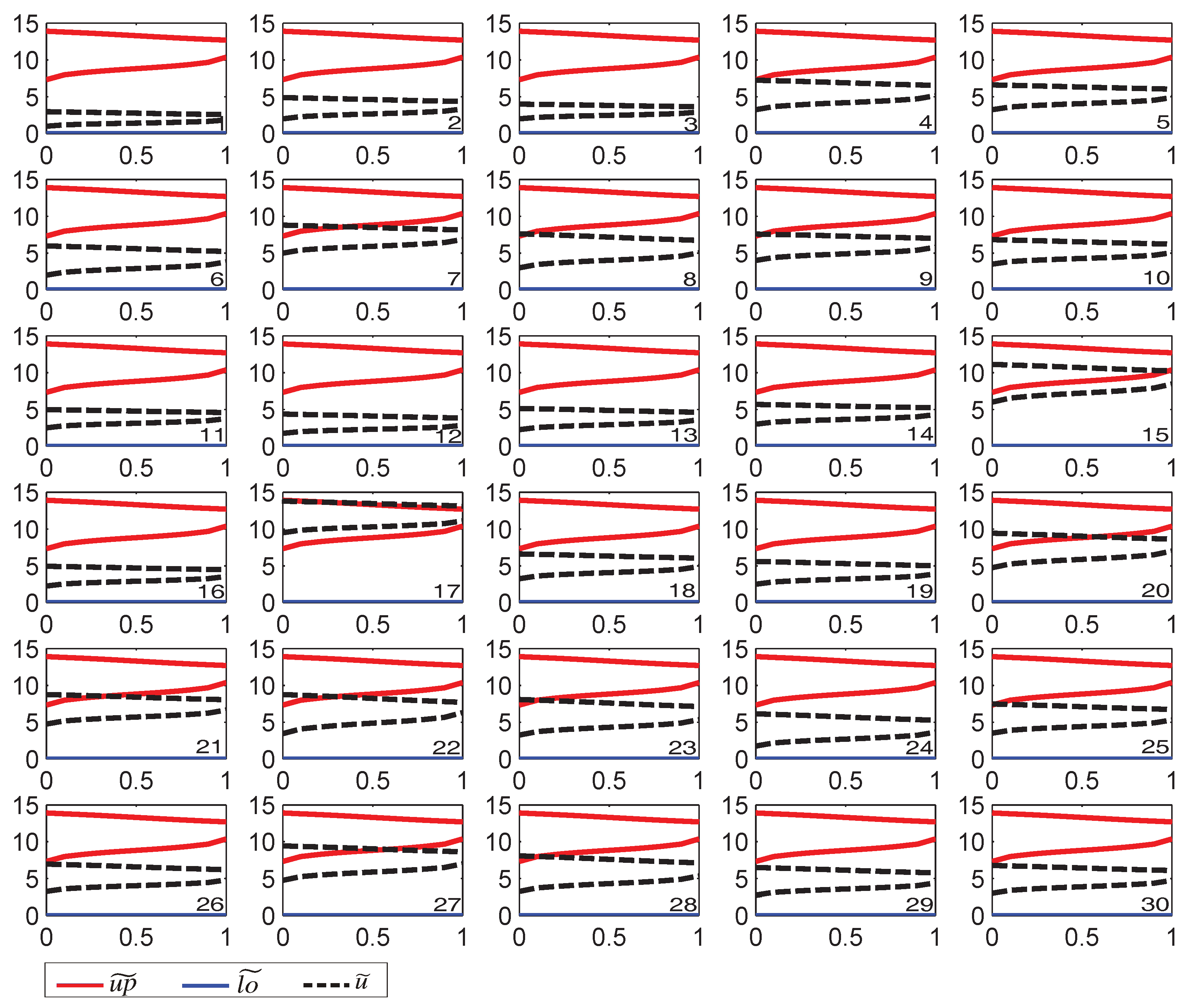
In each sample, four to five rolls of 50 square meters were randomly selected for inspection; and the number of non-conformists of thirty actual observations were recorded.

Table 1. The number of white spots detected.

Sub.	Size		${\mathit{FO}}_{\mathit{i}}$		Sub.	Size		${\mathit{FO}}_{\mathit{i}}$
1	5	1	2	3	16	5	3	4	5
2	4	2	4	5	17	5	10	13	14
3	4	2	3	4	18	4	4	5	6
4	5	3	6	7	19	5	4	5	6
5	5	3	5	6	20	4	5	8	10
6	4	2	5	6	21	4	5	7	8
7	5	5	7	9	22	5	6	7	9
8	4	4	6	7	23	5	4	7	8
9	5	4	6	7	24	5	2	5	6
10	5	4	5	6	25	5	4	6	7
11	5	3	4	5	26	5	4	5	7
12	4	2	3	4	27	5	5	8	9
13	4	3	4	5	28	5	4	6	8
14	5	3	4	5	29	4	3	5	6
15	5	6	10	11	30	4	3	5	7

shows a typical example of white spot data collected from one of the eleven companies. Specifically, each subgroup was appropriately labeled and each quality controller inspected two certain subgroups randomly three times at different intervals. It was found that the number of nonconformists detected each time in the same subgroup was different, indicating that the human subjectivity obviously affects the counting of the dyed defects; thus, the recorded data are considered as fuzzy numbers.

From the data in Table 1, relevant u-chart is constructed as in Figure 3.

5.2. Comparative Analysis

Apparently, the categorization rules shown in Section 4.3 are identical to those of Shu et al. [44]. Here, we perform a comparative analysis between two approaches.

Based on the proposed classification mechanism, the performance of the current dyeing process can be effectively monitored with a u-chart. For brevity, this section displays the classifying results for only five different values $\beta$ = 0.5, 0.6, 0.7, 0.8 as shown in

Table 2. u-Chart classification based on Shu et al.’s [44] approach.

Sub.	0.5	0.6	0.7	0.8	$\mathbf{▵}{\mathit{S}}^{*}$	0.5	0.6	0.7	0.8
1	2.6312	2.6459	2.6606	2.6753	0.0147	In	In	In	In
2	2.2522	2.2657	2.2792	2.2927	0.0135	In	In	In	In
3	2.3114	2.3228	2.3342	2.3456	0.0114	In	In	In	In
4	1.4553	1.4699	1.4845	1.4991	0.0146	In	In	In	In
5	1.6654	1.6739	1.6824	1.6909	0.0085	In	In	In	In
6	1.9181	1.9316	1.9451	1.9586	0.0135	In	In	In	In
7	1.1658	1.1871	1.2084	1.2297	0.0213	In	In	In	In
8	1.4466	1.4641	1.4816	1.4991	0.0175	In	In	In	In
9	1.4144	1.4241	1.4338	1.4435	0.0097	In	In	In	In
10	1.5025	1.5128	1.5231	1.5334	0.0103	In	In	In	In
11	2.2784	2.2999	2.3214	2.3429	0.0215	In	In	In	In
12	2.8702	2.8820	2.8938	2.9056	0.0118	In	In	In	In
13	2.2506	2.2569	2.2632	2.2695	0.0063	In	In	In	In
14	1.9564	1.9685	1.9806	1.9927	0.0121	In	In	In	In
15	0.9199	0.9961	1.0723	1.1485	0.0762	In	In	In	In
16	2.1772	2.1829	2.1886	2.1943	0.0057	In	In	In	In
17	−0.0083	0.0015	0.0113	0.0211	0.0098	R-Out	R-In	In	In
18	1.3923	1.4051	1.4179	1.4307	0.0128	In	In	In	In
19	1.8529	1.8666	1.8803	1.8940	0.0137	In	In	In	In
20	1.1172	1.1283	1.1394	1.1505	0.0111	In	In	In	In
21	1.1382	1.1449	1.1516	1.1583	0.0067	In	In	In	In
22	1.2306	1.2371	1.2436	1.2501	0.0065	In	In	In	In
23	1.4805	1.4894	1.4983	1.5072	0.0089	In	In	In	In
24	1.9884	1.9959	2.0034	2.0109	0.0075	In	In	In	In
25	1.8368	1.8447	1.8526	1.8605	0.0079	In	In	In	In
26	1.8165	1.8217	1.8269	1.8321	0.0052	In	In	In	In
27	1.0131	1.0229	1.0327	1.0425	0.0098	In	In	In	In
28	1.3446	1.3507	1.3568	1.3629	0.0061	In	In	In	In
29	1.4602	1.4695	1.4788	1.4881	0.0093	In	In	In	In
30	1.4558	1.4625	1.4692	1.4759	0.0067	In	In	In	In

Notes: $▵S^{*}=▵D{S}_{i-j}^{▵\beta =0.1}$.

and

Table 3. u-Chart classification based on Nguyen & Hien’s [27] approach.

Sub.	0.5	0.6	0.7	0.8	$\mathbf{▵}{\mathit{N}}^{*}$	0.5	0.6	0.7	0.8
1	3.2995	3.3180	3.3365	3.355	0.0185	In	In	In	In
2	2.8243	2.8415	2.8587	2.8759	0.0172	In	In	In	In
3	2.8985	2.9129	2.9273	2.9417	0.0144	In	In	In	In
4	1.8249	1.8433	1.8617	1.8801	0.0184	In	In	In	In
5	2.0884	2.0991	2.1098	2.1205	0.0107	In	In	In	In
6	2.4053	2.4224	2.4395	2.4566	0.0171	In	In	In	In
7	1.4619	1.4887	1.5155	1.5423	0.0268	In	In	In	In
8	1.8142	1.8363	1.8584	1.8805	0.0221	In	In	In	In
9	1.7737	1.7859	1.7981	1.8103	0.0122	In	In	In	In
10	1.8841	1.8972	1.9103	1.9234	0.0131	In	In	In	In
11	2.8571	2.8842	2.9113	2.9384	0.0271	In	In	In	In
12	3.5992	3.6139	3.6286	3.6433	0.0147	In	In	In	In
13	2.8223	2.8302	2.8381	2.846	0.0079	In	In	In	In
14	2.4533	2.4685	2.4837	2.4989	0.0152	In	In	In	In
15	1.1536	1.2495	1.3454	1.4413	0.0959	In	In	In	In
16	2.7302	2.7374	2.7446	2.7518	0.0072	In	In	In	In
17	−0.0384	−0.0281	−0.0178	−0.0075	0.0103	Out	Out	Out	R-Out
18	1.7459	1.7621	1.7783	1.7945	0.0162	In	In	In	In
19	2.3235	2.3407	2.3579	2.3751	0.0172	In	In	In	In
20	1.4012	1.4154	1.4296	1.4438	0.0142	In	In	In	In
21	1.4273	1.4357	1.4441	1.4525	0.0084	In	In	In	In
22	1.5432	1.5514	1.5596	1.5678	0.0082	In	In	In	In
23	1.8565	1.8677	1.8789	1.8901	0.0112	In	In	In	In
24	2.4935	2.5029	2.5123	2.5217	0.0094	In	In	In	In
25	2.3033	2.3131	2.3229	2.3327	0.0098	In	In	In	In
26	2.2779	2.2844	2.2909	2.2974	0.0065	In	In	In	In
27	1.2704	1.2828	1.2952	1.3076	0.0124	In	In	In	In
28	1.6861	1.6938	1.7015	1.7092	0.0077	In	In	In	In
29	1.8311	1.8428	1.8545	1.8662	0.0117	In	In	In	In
30	1.8256	1.8340	1.8424	1.8508	0.0084	In	In	In	In

Notes: $▵N^{*}=▵D{S}_{i-j}^{▵\beta =0.1}$.

. We can observe that twenty-nine out of the thirty subgroups investigated are considered in-control at these optimism levels. For a comparative analysis between Shu et al. [44] and Nguyen and Hien [27] in this case, both approaches all show a warning signal at the 17th subgroup. While the former classifies the sample as rather out-of-control at the optimism level of 0.5, rather in-control at 0.6 and in-control if the optimism level is larger than 0.6, the latter classifies it as out-of-control for the optimism level less than 0.8 and rather out-of-control at the level of 0.8. It implies that in this case Nguyen and Hien’s [27] approach provides a more discriminatory power.

These results also indicate that for more optimistic decision-makers, the process is more likely to be considered in statistical control. This finding shows that the evaluation of the dyed quality or the process status is critically affected by human behavior, i.e., the level of optimism. More importantly, an investigation is also conducted to look for the assignable causes occurred in the production of the mentioned sample. Once the significant causes are found, having proper corrective actions undertaken to either eliminate or reduce their negative impacts can greatly improve the cloth dyeing quality.

6. Conclusions

In several industrial manufacturing industries, the existence of errors in measurement systems and the human subjectivity in decision-making process makes the collected data imprecise, also called fuzzy data. Consequently, in the fuzzy environment, traditional Shewhart-type control charts turn out to be inappropriate because they require crisp data to categorize manufacturing process conditions.

In this paper, the fuzzy u-chart is constructed to monitor the fuzzy average number of nonconformities per unit. Its fuzzy control limits are first obtained based on the results of the resolution-identity theorem. Moreover, in order to monitor the process based on the fuzzy control chart, we first extend a recent developed fuzzy ranking method proposed by Nguyen and Hien [27]. The ranking strategy is based on the quantity of fuzzy numbers’ left-right areas and centroids to provide more satisfactory reasoning. Then thorough evaluation rules are established to classify the manufacturing process with four different linguistic states, including In-control, Out-of-control, Rather out-of control and Rather in-control. Basically, the incorporation of optimism level into the ranking index provides critical flexibility in decision-making procedure, so decision-makers can exert their savvy experiences in implementing proper actions to fully control the quality of manufactured products. In the empirical case study of Vietnam textile dyeing industry, the results show that the deployment of our proposed fuzzy u-chart can be of great benefit in early detecting the occurrence of assignable causes.

Finally, as to some extent of anomalous conditions is monitored, this intermediate classification mechanism can provide critical information to determine whether a further action taken is required by contemplating the intervention cost as opposed to the quality gain. Thus, this approach can obviously avoid not only unnecessary adjustment to the current process but also the potential loss in their business. As such, our proposed fuzzy u-chart can fulfill the current literature of the conventional u-chart in terms of effectiveness when fuzzy data is inevitably present in the manufacturing process.

References

- Montgomery, D.C. Statistical Quality Control—A Modern Introduction; Wiley & Sons: Singapore, 2013. [Google Scholar]
- Walpole, R.E.; Myers, R.H.; Myers, S.L.; Ye, K. Probability and Statistics for Engineers and Scientists, 9th ed.; Prentice Hall: Boston, MA, USA, 2012. [Google Scholar]
- Evans, J.R.; Lindsay, W.M. The Management and Control of Quality, 8th ed.; South-Western College Publishing: New York, NY, USA, 2011. [Google Scholar]
- Shu, M.H.; Nguyen, T.L.; Hsu, B.M. Fuzzy MaxGWMA chart for identifying abnormal variations of on-line manufacturing processes with imprecise information. Expert Syst. Appl. 2014, 41, 1342–1356. [Google Scholar] [CrossRef]
- Lu, K.P.; Chang, S.T.; Yang, M.S. Change-point detection for shifts in control charts using fuzzy shift change-point algorithms. Comput. Ind. Eng. 2016, 93, 12–27. [Google Scholar] [CrossRef]
- Ghobadi, S.; Noghodarian, K.; Noorossana, R.; Mirhosseini, S.M. Developing a multivariate approach to monitor fuzzy quality profiles. Qual. Quant. 2012. [Google Scholar] [CrossRef]
- Gülbay, M.; Kahraman, C.; Ruan, D. α-cut fuzzy control charts for linguistic data. Int. J. Intell. Syst. 2004, 19, 1173–1196. [Google Scholar] [CrossRef]
- Hsieh, C.S.; Chen, Y.W.; Wu, C.H. Characteristics of fuzzy synthetic decision methods for measuring student achievement. Qual. Quant. 2012, 46, 523–543. [Google Scholar] [CrossRef]
- Senturk, S.; Erginel, N. Development of fuzzy and control charts using α-cuts. Inf. Sci. 2009, 179, 1542–1551. [Google Scholar] [CrossRef]
- Faraz, A.; Shapiro, A.F. An application of fuzzy random variables to control charts. Fuzzy Sets Syst. 2010, 161, 2684–2694. [Google Scholar] [CrossRef]
- Faraz, A.; Moghadam, M.B. Fuzzy control chart a better alternative for Shewhart average chart. Qual. Quant. 2007, 41, 375–385. [Google Scholar] [CrossRef]
- Gülbay, M.; Kahraman, C. Development of fuzzy process control charts and fuzzy pattern analyses. Comput. Stat. Data Anal. 2006, 51, 434–451. [Google Scholar] [CrossRef]
- Gülbay, M.; Kahraman, C. An alternative approach to c-fuzzy control charts: direct fuzzy approach. Inf. Sci. 2007, 177, 1463–1480. [Google Scholar] [CrossRef]
- Shu, M.H.; Wu, H.C. Fuzzy and R control charts: Fuzzy dominance approach. Comput. Ind. Eng. 2011, 61, 676–685. [Google Scholar] [CrossRef]
- Nguyen, T.L.; Hsu, B.M.; Shu, M.H. New quantitative approach based on index of optimism for fuzzy judgement of online manufacturing process. Mater. Res. Innov. 2014, 18, 2–4. [Google Scholar] [CrossRef]
- Morabia, Z.S.; Owliaa, M.S.; Bashirib, M.; Doroudyana, M.H. Multi-objective design of control charts with fuzzy process parameters using the hybrid epsilon constraint PSOs. Appl. Soft Comput. 2015, 30, 390–399. [Google Scholar] [CrossRef]
- Wang, J.H.; Raz, T. On the construction of control charts using linguistic variables. Int. J. Prod. Res. 1990, 28, 477–487. [Google Scholar] [CrossRef]
- Kanagawa, A.; Tamaki, F.; Ohta, H. Control charts for progress average and variability based on linguistic data. Int. J. Prod. Res. 1993, 31, 913–922. [Google Scholar] [CrossRef]
- Laviolette, M.; Seaman, J.W.; Barrett, J.D.; Woodall, W.H. A probabilistic and statistical view of fuzzy methods, with discussions. Technometrics 1995, 37, 249–292. [Google Scholar] [CrossRef]
- Asai, K. Fuzzy Systems for Management; IOS Press: Amsterdam, The Netherlands, 1995. [Google Scholar]
- Woodall, W.; Tsui, K.L.; Tucker, G.L. A Review of statistical and fuzzy control charts based on categorical data. In Frontiers in Statistical Quality Control 5; Lenz, H.J., Wilrich, P.T., Eds.; Physica: Heidelberg, Germany, 1997. [Google Scholar]
- Cheng, C.B. Fuzzy process control: Construction of control charts with fuzzy numbers. Fuzzy Sets Syst. 2005, 154, 287–303. [Google Scholar] [CrossRef]
- Guo, R.; Zhao, R.; Cheng, C. Quality control charts for random fuzzy manufacturing environments. J. Qual. 2008, 15, 101–115. [Google Scholar]
- Grzegorrzewski, P.; Hryniewicz, O. Soft methods in statistical quality control. Control Cybern. 2000, 29, 119–140. [Google Scholar]
- Chien, C.F.; Chen, J.H.; Wei, C.C. Constructing a comprehensive modular fuzzy ranking framework and illustrations. J. Qual. 2011, 18, 333–349. [Google Scholar]
- Nguyen, T.L.; Shu, M.H.; Huang, Y.F.; Hsu, B.M. Fuzzy and s charts: Left & Right dominance approach. In Advanced Methods for Computing Collective Intelligence; Nguyen, N.T., Trawiński, B., Katarzyniak, R., Jo, G.S., Eds.; Springer: Berlin/Heidelberg, Germany, 2013; pp. 355–366. [Google Scholar]
- Nguyen, T.L.; Hien, L.T. Innovatively ranking fuzzy numbers with left-right areas and centroids. J. Inf. Math. Sci. 2016, 8, 167–174. [Google Scholar]
- Shu, M.H.; Dang, D.C.; Nguyen, T.L.; Hsu, B.M. Fuzzy and s control charts: A data-adaptability and human-acceptance approach. Complexity 2017. [Google Scholar] [CrossRef]
- Zadeh, L.A. Fuzzy sets. Inf. Control 1965, 8, 338–353. [Google Scholar] [CrossRef]
- Wu, H.C. Evaluate fuzzy Riemann integrals using the Monte Carlo method. J. Math. Anal. Appl. 2001, 264, 324–343. [Google Scholar] [CrossRef]
- Wu, H.C. Fuzzy estimation on lifetime data. Comput. Stat. 2004, 19, 613–633. [Google Scholar] [CrossRef]
- Yu, V.F.; Chi, H.T.X.; Chen, C.W. Ranking fuzzy numbers based on epsilon-deviation degree. Appl. Soft Comput. 2013, 13, 3621–3627. [Google Scholar] [CrossRef]
- Yu, V.F.; Chi, H.T.X.; Dat, L.Q.; Phuc, P.N.K.; Chen, C.W. Ranking generalized fuzzy numbers in fuzzy decision making based on left and right transfer coefficients and areas. Appl. Math. Model. 2013, 37, 8106–8117. [Google Scholar] [CrossRef]
- Yu, V.F.; Dat, L.Q. An improved ranking method for fuzzy numbers with integral values. Appl. Soft Comput. 2014, 14, 603–608. [Google Scholar] [CrossRef]
- Nejad, A.M.; Mashinchi, M. Ranking fuzzy numbers based on the areas on the left and the right sides of fuzzy number. Comput. Math. Appl. 2011, 61, 431–442. [Google Scholar] [CrossRef]
- Wang, Y.M.; Luo, Y. Area ranking of fuzzy numbers based on positive and negative ideal points. Comput. Math. Appl. 2009, 58, 1769–1779. [Google Scholar] [CrossRef]
- Singh, P. A new approach for the ranking of fuzzy sets with different heights. J. Appl. Res. Technol. 2012, 10, 941–949. [Google Scholar]
- Phuc, P.N.K.; Yu, V.F.; Chou, S.Y.; Dat, L.Q. Analyzing the ranking method for L-R fuzzy numbers based on deviation degree. Comput. Ind. Eng. 2012, 63, 1220–1226. [Google Scholar] [CrossRef]
- Chu, T.C.; Tsao, C.T. Ranking fuzzy numbers with an area between the centroid point and original point. Comput. Math. Appl. 2002, 43, 111–117. [Google Scholar] [CrossRef]
- Mitchell, H.B.; Schaefer, P.A. On ordering fuzzy numbers. Int. J. Intell. Syst. 2000, 15, 981–993. [Google Scholar] [CrossRef]
- Wong, W.K.; Yuen, C.W.M.; Fan, D.D.; Chan, L.K.; Fung, E.H.K. Stitching defect detection and classification using wavelet transform and BP neural network. Expert Syst. Appl. 2009, 36, 3845–3856. [Google Scholar] [CrossRef]
- Yuen, C.W.M.; Wong, W.K.; Qian, S.Q.; Chan, L.K.; Fung, E.H.K. A hybrid model using genetic algorithm and neural network for classifying garment defects. Expert Syst. Appl. 2009, 36, 2037–2047. [Google Scholar] [CrossRef]
- Lee, C.K.H.; Choy, K.L.; Ho, G.T.S.; Chin, K.S.; Law, K.M.Y.; Tse, Y.K. A hybrid OLAP-association rule mining based quality management system for extracting defect patterns in the garment industry. Expert Syst. Appl. 2013, 40, 2435–2446. [Google Scholar] [CrossRef]
- Shu, M.H.; Chiu, C.C.; Nguyen, T.L.; Hsu, B.M. A demerit-fuzzy rating system, monitoring scheme and classification for manufacturing processes. Expert Syst. Appl. 2014, 41, 7878–7888. [Google Scholar] [CrossRef]
Figure 1.
Left and right areas of .
Figure 2.
Common defects in dyed cloth. (a) Cloudy; (b) Shade variation; (c) Tonal variation; (d) Poor light fastness; (e) Dyed stain; (f) Color crocking; (g) White spot; (h) White spot.
Figure 3.
u-Chart for monitoring the white spots in dyed cloth.