Single Image Super-Resolution by Non-Linear Sparse Representation and Support Vector Regression

Abstract

Sparse representations are widely used tools in image super-resolution (SR) tasks. In the sparsity-based SR methods, linear sparse representations are often used for image description. However, the non-linear data distributions in images might not be well represented by linear sparse models. Moreover, many sparsity-based SR methods require the image patch self-similarity assumption; however, the assumption may not always hold. In this paper, we propose a novel method for single image super-resolution (SISR). Unlike most prior sparsity-based SR methods, the proposed method uses non-linear sparse representation to enhance the description of the non-linear information in images, and the proposed framework does not need to assume the self-similarity of image patches. Based on the minimum reconstruction errors, support vector regression (SVR) is applied for predicting the SR image. The proposed method was evaluated on various benchmark images, and promising results were obtained.

1. Introduction

Single image super-resolution (SISR) techniques try to enhance the resolution of an image with low resolution (LR) to obtain an image with high resolution (HR). Meanwhile, SISR also tries to alleviate the effects brought by visual artifacts. There are three types of SISR techniques: interpolation-based, reconstruction-based and learning-based. The interpolation-based techniques [1] are fast. However, the drawback of these types of techniques is that they tend to blur the fine details in images. For the reconstruction-based techniques [2,3], the self-similarity of image patches are often required. Each patch of the HR image can then be synthesized by similar patches in the LR image(s). The learning-based methods [4,5,6] (also called example-based methods) model image details from a training dictionary of LR/HR images or patch pairs. Nevertheless, these types of methods tend to strongly rely on the trained dictionary in order to obtain satisfactory results.

In recent years, sparse representation of signals has become an important tool in computer vision. In many applications in computer vision, such as image denoising, image super-resolution and object recognition, sparse representations have produced remarkable performance [7,8,9]. It has also been verified that sparse representation or sparse coding can achieve good outcomes in many image classification tasks [10,11,12]. The reason for the success of sparse coding is that a signal Y can be well represented by a linear combination of a sparse vector x and a given dictionary D, namely, if x and D can be properly found, then Y can be well approximated as: $Y\approx Dx$.

There are two methods to help obtain a dictionary for sparse representation: using an existing dictionary and dictionary learning. Using an existing dictionary means to choose a pre-computed basis such as a wavelet basis and a curvelet basis. However, in different computer vision tasks, better image representations can be expected with task-specific dictionaries learnt from given sample images [13].

Many algorithms have been proposed to tackle the problem of dictionary learning, the method of optimal directions (MOD) [14] and the KSVD algorithm [15] are two of the most well-known methods. The dictionaries learned by MOD and KSVD are linear representations of the data. However, in many computer vision applications, one has to face non-linear distributions of the data, using a linear dictionary learning model often leads to poor performance. Therefore, several non-linear dictionary learning methods have been proposed. Among them, a recently proposed method kernel KSVD (KKSVD) [16] has shown its ability to obtain better image description than the linear models. The kernel KSVD includes two steps: sparse coding and dictionary update. In a sparse coding stage, the Kernel Orthogonal Matching Pursuit (KOMP) is used for seeking the sparse coefficients. Once the sparse coefficients are obtained, the kernerlized KSVD is then used in the second stage for a dictionary update. It is demonstrated that the kernel KSVD can provide better image classification performance than the traditional linear dictionary learning models.

Although the kernel KSVD can outperform its linear counterparts by introducing the non-linear learning procedure, the learned sparse vector and the dictionary still comprise both additive and subtractive interactions. From the perspective of biological modeling, the existence of both the additive and subtractive elements in the sparse representations of signals is contrary to the non-negativity of neural firing rates [17,18]. Moreover, the negative and positive elements in the representations may induce the ‘cancel each other out’ phenomenon, which is contrary to the intuitive notion of combining non-negative representations [19]. Therefore, many researchers have claimed to use non-negative sparse representations in vision-related applications [20,21]. The non-negative sparse representations are based on the constraints that the input data Y, the dictionary D, and the sparse vector x are all non-negative.

The non-negative sparse representation has been successfully applied in many computer vision applications, such as face recognition [20,22], motion extraction [22,23], image classification and retrieval [24,25]. Nevertheless, these non-negative sparse representations are all based on linear learning models. Therefore, their ability to capture the non-linear distributions of data is limited.

Inspired by the success of sparse coding in signal processing applications, sparse coding has also recently been used for single image super-resolution. In many existing sparsity-based SR methods such as [5,26], it is assumed that the sparse representation of high resolution image patches can be recovered from the low resolution image patches. However, the training image patches must be carefully selected, which means that their methods only work for images that have similar statistical nature.

Motivated by this drawback of the existing sparse representation models, in this paper, we propose using a non-linear sparse representation model for single image super-resolution. The non-linear sparse model is first used to learn non-linear dictionaries from low resolution images, and then support vector regression (SVR) is applied for predicting the pixels in the target high resolution image. Unlike the aforementioned sparsity-based SR methods, the non-linear sparse model is used here for dictionary learning.

In our proposed method, we employ the same scheme in [27,28], in which the input image is down-sampled by several different scales. For each image in every scale, the image patches are separated into the ‘low-frequency’ and ‘high-frequency’ categories, and then sparse representation methods are used to describe image patches. Different from the existing sparsity-based methods, in this paper, a novel non-negative and non-linear sparse representation model is proposed and used for describing the image patches.

In the proposed sparse model, in the sparse coding stage, a kernerlized iterative rule is proposed to obtain the coefficient matrix. In the dictionary learning stage, the kernel KSVD algorithm is used to learn the dictionary. In order to keep the non-negativity, a simple method is proposed to update the learned dictionary elements.

Once the sparse representation of an image patch in the input image is obtained, it can be used to reconstruct the corresponding image patches in different scales. The image patch which produces the minimum reconstruction error is more appropriate for the refinement of the image patch, i.e., it will be used for the super-resolution. The support vector regression is used here for this patch selecting procedure.

The rest of the paper is organized as follows. In Section 2, related work in SR is introduced. Section 3 details our proposed single image super-resolution framework. Experimental results and discussion are given in Section 4. Finally, Section 5 concludes the paper.

2. Related Work

In the past few years, the sparse representation based SR methods have received much attention. The sparse representation technique was first utilized in SR by Yang et al. [26]. The authors suggested that the sparse representation of high resolution images can be recovered from the low resolution image patches. However, their method usually suffers from inconsistency between neighboring patches. Therefore, priors of image self-similarities and local/nonlocal regularities were proposed to produce more robust prediction. In [4], the authors investigated the non-local self-similarity within and across spatial scales. Once similar patches are found in different scaled versions, the SR image can be synthesized by classical SR methods such as [2]. Later, Yang et al. [29] extended the framework of [4]. In their work, the high and low-resolution image pairs from the image pyramid are concatenated, and the sparse representation of the pairs is jointly learned. For an LR image patch, similar patches are searched in the image pyramid, and the jointly learned sparse representation is used for estimating the final SR result. A learning-based single image SR method is proposed in [5], and the high resolution image is obtained by using sparse regression and natural image priors. However, additional techniques are required to remove the blurring and ringing effects near the edges in the SR result image.

Recently, there has been a trend in SR to combine the example-based and reconstruction-based methods for producing more compelling results [30,31]. In the combined methods, the mapping from LR images to HR images is viewed as a regression problem: the reconstruction-based techniques are used to learn the bases (dictionaries) from the input LR image itself, and a regression model is then used for predicting pixels in the corresponding HR image.

Many methods have been applied to obtain an appropriate dictionary. Traditional options are some pre-computed methods such as wavelet or curvelet bases. However, these pre-designed bases often lack flexibility to a randomly given image. Instead, people propose using dictionaries learned from images. The techniques used for learning a dictionary include methods such as PCA [31], KSVD [15,32] and MOD [14]. The dictionaries learned by these methods are linear representations of the data. However, in many computer vision applications, one has to face non-linear distributions of the data. Using a linear dictionary learning model often leads to poor performance. Therefore, several non-linear dictionary learning methods have been proposed and have outperformed their linear counterparts in some computer vision tasks such as image classification [16]. It gives a hint that using a non-linear dictionary learning model in SR tasks may also produce better performance than linear models.

In terms of regression models, many have been utilized in SR tasks. Examples include Gaussian process regression (GPR) [6], kernel ridge regression (KRR) [5] and SVR [33]. Among them, SVR is a widely used regression method in SR, which exhibits excellent generalization ability in predicting functional outputs without any prior knowledge or assumption on the training data [30]. This property of SVR fits our proposed method well, as, in our method, we do not need to train LR and HR image pairs in advance.

3. Proposed Method

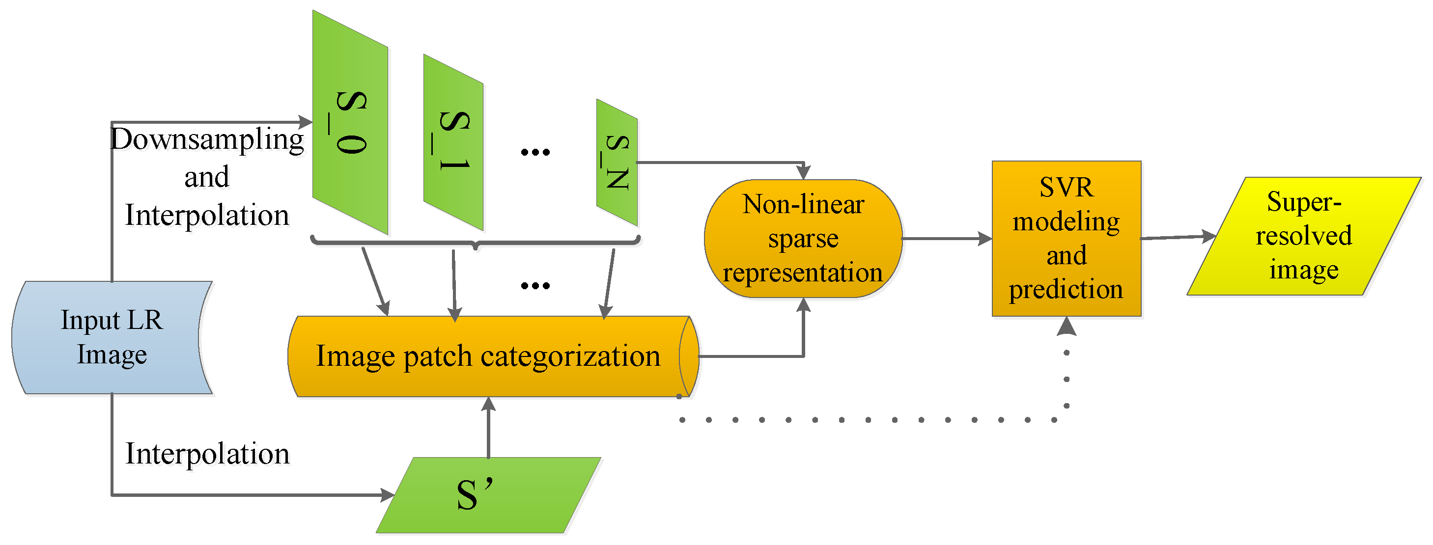
The proposed single image SR method is presented in this section. The main framework of our proposed method can be seen in Figure 1, where the input LR image is first downsampled with several factors to obtain several images in different scales. Then, a classical interpolation method such as bicubic interpolation can be used for each image to produce the $S_0$,…,$S_N$ in the figure. For each image of {$S_0$,…,$S_N$}, image patches are extracted and categorized as ‘high frequency’ or ‘low frequency’. Then, the non-linear sparse representation is utilized to represent each image patch. Meanwhile, the original input image is directly interpolated to produce a high resolution image $S^{\prime }$. The image patches extracted from $S^{\prime }$ will later be used for predicting the final SR result (the dot line in Figure 1).

In previous sparsity-based methods such as [8,10], the sparse model is trained by using a small number of randomly selected image patches, and this indicates that their methods may only be effective on those images that contain similar structures. Example-based methods such as [5,29] may produce artifacts around the edges. To tackle the problem, further processing techniques are needed. To solve the aforementioned problems, some researchers proposed treating the salient regions (especially edge regions) and the smooth regions separately. Using image segmentation techniques such as widely used edge detectors, image patches can be labelled as different types such as ‘high frequency’ (patches contain edge pixels) and ‘low frequency’ (smooth patches). Different learning models thus can be built for different types of image patches. During the image refinement stage, different models then can be selected for different types of image patches in the input image. The technique of categorization of image patches obtained promising results in some SISR tasks [28,30,34]. In this paper, the technique of categorization of image patches is also used.

The learned non-linear sparse representation of image patches is then used to establish the SVR models. Finally, the obtained SVR models are used for selecting the best candidate patch in {$S_0$,…,$S_N$} for the refinement of each image patch in $S^{\prime }$ to generate the final SR image.

It can be noted that the proposed method employs the same scheme in [27,28,30], in which the ‘low-frequency’ and ‘high-frequency’ image patches are used for learning, and support vector regression is used for image refinement. However, in our method, a novel non-negative and non-linear sparse representation model is proposed and used for describing the image patches.

3.1. Non-Linear Sparse Representation

The non-negative sparse coding (NNSC) stresses both the non-negativity and sparseness for data representation. Therefore, given a set of data Y, the NNSC can be defined as the following minimization problem:

$$\begin{array}{cc}& \underset{D,X}{argmin}{\parallel Y-DX\parallel }^{2}s.t.,\hfill \\ & \parallel x_i{\parallel }_0\le T,\parallel d_j{\parallel }_2=1.D_{ij}\ge 0,X_{ij}\ge 0,\forall i,j,\hfill \end{array}$$

(1)

where X is the sparse matrix containing sparse vectors, and D is the dictionary.

In an NNSC data representation procedure, the first stage is to optimize the sparse matrix X. The global minimization can be obtained by quadratic programming or gradient descent. In [19], a multiplicative algorithm was proposed for obtaining the sparse matrix. The algorithm can be described as the following iterative update rule:

$$X^{t+1}=X^t\odot \left(D^{T}Y\right)./(D^{T}D{X}^t+\lambda ),$$

(2)

where ⊙ and $./$ denote element-wise multiplication and division, respectively. λ is the tradeoff between sparseness and accurate reconstruction, and a typical choice is $\lambda =\left|x\right|$, where x is a vector in the sparse matrix X. The scalar λ is added to every element of the matrix $D^{T}D{X}^t$.

In the second stage, the dictionary D is learned. The obtained sparse matrix X is fixed here. Then, D can be obtained by dictionary learning algorithms. For example, Hoyer [19] proposed a gradient descent based algorithm to learn the dictionary with a non-negative constraint. Other dictionary learning algorithms can also be used for updating D. However, the non-negative constraints must be considered to keep the non-negativity of the learned dictionary. The aforementioned two stages of NNSC are iteratively processed in turn for updating the sparse matrix and the dictionary, respectively.

Unlike the prior sparsity-based SR methods, the non-linear sparse representation is used here. The main idea of the kernel KSVD is briefly introduced in this section. The kernelized KSVD [16] is used for image patch feature representation, as it was investigated in [16], that the kernelized KSVD outperforms kernelized MOD and kernel PCA in the experimental image analysis applications.

The goal of kernel dictionary learning is to obtain a non-linear dictionary $D=[d_1,\dots ,d_k]$ in a Hilbert space $\mathcal{F}$. Define $\varphi :{\mathbb{R}}^n\to \mathcal{F}\in {\mathbb{R}}^m$ as a non-linear mapping from ${\mathbb{R}}^n$ to a Hilbert space $\mathcal{F}$, where $m\gg n$. To obtain the non-linear dictionary D, one has to solve the following optimization problem:

$$\underset{D,X}{argmin}{\parallel \varphi \left(Y\right)-DX\parallel }_F^{2}s.t.\parallel x_i{\parallel }_0\le T,\parallel d_j{\parallel }_2=1,\forall i,j,$$

(3)

where $\parallel ·{\parallel }_F$ is the Frobenius norm of a matrix, for a matrix M has the dimension of $m\times n$, and it can be obtained as: $\parallel M{\parallel }_F={({\sum }_{i=1}^m{\sum }_{j=1}^{n}M{(i,j)}^2)}^{\frac{1}{2}}$. $\varphi \left(Y\right)=[\varphi \left(Y_1\right),\varphi \left(Y_2\right),\dots ,\varphi \left(Y_n\right)]$. $X\in {\mathbb{R}}^{k\times n}$ is a sparse matrix, and each column $x_i$ in X is a sparse vector that has a maximum of T non-zero elements.

The dimension of the Hilbert space $\mathcal{F}$ can possibly be infinite. Therefore, the traditional dictionary learning methods such as KSVD and MOD are incapable of the optimization task. In order to tackle the optimization problem in Equation (3), the kernel KSVD (KKSVD) dictionary learning [16] was proposed. KKSVD consists of two stages. First, the kernel orthogonal matching pursuit (KOMP) is used for sparse coding. Then, the kernel KSVD is used for a dictionary update.

In the sparse coding stage, by introducing kernel mapping, the problem in Eqquation (3) can be rewritten as:

$$\parallel \varphi \left(Y\right)-\varphi \left(Y\right)AX{\parallel }_F^2=\sum _{i=1}^N\parallel \varphi \left(y_i\right)-\varphi \left(Y\right)A{x}_i{\parallel }_2^2.$$

(4)

Note the dictionary D in Equation (3) is changed to a coefficient matrix, A, as it is proved that there exists an optimal solution $D^{*}$, which has the form $D^{*}=\varphi \left(Y\right)A$. [16].

Therefore, now the problem in Equation (4) can be solved by any pursuit algorithms. For example, a kernelized version of the orthogonal matching pursuit algorithm (OMP) [35] is used in [16]. In the sparse coding stage, the coefficient matrix A is fixed and the KOMP algorithm can be used to search for the sparse matrix X. The details of the KOMP algorithm can be found in [16].

In the dictionary update stage, the kernel KSVD is used. Let $a_k$ and $x_T^j$ represent the k-th column and the j-th row of A and X, respectively. The approximation error:

$$\parallel \varphi \left(Y\right)-\varphi \left(Y\right)AX{\parallel }_F^2$$

(5)

can be written as:

$$\begin{array}{cc}\hfill & {∥\varphi \left(Y\right)-\varphi \left(Y\right)\sum _{j=1}^K{\alpha }_j{x}_T^j∥}_F^2\hfill \\ \hfill =& {∥\varphi \left(Y\right)\left(I-\sum _{j\ne k}{\alpha }_j{x}_T^j\right)-\varphi \left(Y\right)\left({\alpha }_k{x}_T^k\right)∥}_F^2\hfill \\ \hfill =& \parallel \varphi \left(Y\right)E_k-\varphi \left(Y\right)M_k{\parallel }_F^2,\hfill \end{array}$$

(6)

where $E_k=(I-{\sum }_{j\ne k}{a}_j{x}_T^j)$, $M_k=a_k{x}_T^k$. $\varphi \left(Y\right)E_k$ demonstrates the distance between the true signals and the estimated signals when removing the k-th dictionary atom, while $\varphi \left(Y\right)M_k$ specifies the contribution of the k-th dictionary atom to the estimated signals.

In the dictionary update stage, as $E_k$ is a constant for each k, the minimization of Equation (6) is indeed to find the best $a_k$ and $x_T^k$ for the rank-1 matrix $\varphi \left(Y\right)M_k$ to produce the best approximation of $\varphi \left(Y\right)E_k$. Using a singular value decomposition (SVD), one can obtain the solution. However, it is impossible to directly use SVD in this scenario. Using SVD here may greatly increase the number of non-zero elements in X. Moreover, the matrix may have infinitely large row dimensions, which is computationally prohibitive.

Instead of working on all columns of $M_k$, one can only work on a subset of columns, as there is a fact that the columns of $M_k$ associated with the zero-elements in $x_T^k$ are all zero, and these columns do not affect the objective function. Therefore, these zero columns can be discarded and only the non-zero elements in $x_T^k$ are allowed to vary. Therefore, the sparsities are preserved [15].

Let $S_k$ be the set of indices of the signals $\left\{\varphi \left(y_i\right)\right\}$ that use the dictionary atom ${\left(\varphi \left(Y\right)A\right)}_k$. Then, $S_k$ can be defined as:

$$S_k=\left\{i\right|1\le i\le N,x_T^k\ne 0\}.$$

(7)

Denote ${\Gamma }_k$ as a matrix of size $N\times |S_k|$. It has ones on the $(S_k\left(i\right),i)$-th entries and zeroes elsewhere. Using $x_T^k$ multiplies ${\Gamma }_k$, by discarding zeroes, $x_T^k$ will have the length of $|S_k|$. Then, the $E_k$ and $M_k$ in Equation (6) are changed to:

$$E_k^R=E_k{\Gamma }_k;M_k^R=M_k{\Gamma }_k.$$

(8)

By applying SVD decomposition, one can get:

$${\left(E_k^R\right)}^T\mathcal{K}(Y,Y)\left(E_k^R\right)=V\Delta V^T,$$

(9)

where $\mathcal{K}(Y,Y)$ is a positive semidefinite matrix $\left[{\mathcal{K}}_{ij}\right]=\left[\kappa (y_i,y_j)\right]$, and $\kappa (·,·)$ is a mercer kernel defined as $\kappa (x,y)=<\varphi \left(x\right),\varphi \left(y\right)>$. $\Delta ={\Sigma }^T\Sigma$, ${\sigma }_1=\sqrt{\Delta (\mathbf{1},\mathbf{1})}$. Using an iterative procedure, in each iteration, $a_k$ can be updated as:

$$a_k={\sigma }_1^{-1}{E}_k^R{v}_1,$$

(10)

where $v_1$ is the first vector of V corresponding to the largest singular value ${\sigma }_1^2$ in Δ.

The coefficient vector $x_R^k$ is updated as:

$$x_R^k={\sigma }_1{v}_1^T.$$

(11)

For the overall procedure, in the first stage, the KOMP algorithm is used for sparse coding. Then, the KSVD is used in the second stage for dictionary update. The aforementioned two stages are repeated until a stopping criterion is met.

3.2. Non-Negative Kernel KSVD Model

Based on the introduced kernel KSVD model, in this section, the proposed non-negative kernel KSVD model is discussed.

For some applications such as image recognition, using sparse representations and overcomplete dictionaries together with forcing non-negativity on both the dictionary and the coefficients, the learned sparse vectors and the dictionary still comprise only additive elements. This may lead to the ‘ingredient’ form, and all of the training samples are built as an ‘ingredient’ of image contents [18]. With the non-negative constraint, the dictionary atoms become sparser and converge to the building blocks of the training samples [36]. However, the existing non-negative sparse models are all based on linear learning algorithms, and their inability to capture the non-linear data distribution inspires us to embed the non-negativity into the non-linear sparse models.

Although there are other non-linear dictionary learning models such as kernel MOD or kernel PCA can be selected for our task, we prefer to use the kernel KSVD, as in [16], and the authors have demonstrated that the kernel KSVD outperforms other non-linear models in image classification tasks. As we try to make the kernel KSVD produce the non-negative dictionaries and coefficient matrices, it is necessary to vary the original kernel KSVD model. With the non-negative and non-linear constraints, the goal of the sparse coding is now changed to:

$$\underset{X}{min}\parallel \varphi \left(Y\right)-\varphi \left(Y\right)AX\parallel s.t.X\ge 0.$$

(12)

In the sparse coding stage, a pursuit algorithm should be used in order to keep the coefficients non-negative. In [18], an iterative method for non-negative sparse coding is introduced:

$$x^{t+1}=x^t.\odot \left(D^{T}y\right)./(D^{T}D{x}^t+\lambda ),$$

(13)

where t represents the iteration number. $.\odot$ and $./$ represent entry-wise multiplication and division. However, this iterative rule is designed for linear coding. In order to use it in the non-linear scenarios, using the kernel trick, Equation (13) can be varied as:

$$\begin{array}{ccc}{x}^{t+1}\hfill & =\hfill & x^t.\odot ({\left(\varphi \left(Y\right)A\right)}^T\varphi \left(Y\right))./({(\varphi \left(Y\right)A)}^T\left(\varphi \left(Y\right)A\right)x^t+\lambda )\hfill \\ & =\hfill & x^t.\odot \left(A^T\mathcal{K}(Y,Y)\right)./(A^T\mathcal{K}(Y,Y)A{x}^t+\lambda ).\hfill \end{array}$$

(14)

It can also be proven that using the iterative update rule in Equation (14), the objective Equation (12) is non-increasing. Moreover, it is guaranteed that x can still be non-negative using this update rule, as the elements in x are updated by simply multiplying with some non-negative factors.

In the dictionary update stage, the dictionary atoms must be kept non-negative as well. Using the same techniques of the kernel KSVD, under the non-negative constraint, the minimization problem in Equation (6) now has been changed to:

$$\underset{a_k,x_R^k}{min}\parallel \varphi \left(Y\right)E_k^R-\varphi \left(Y\right)a_k{x}_R^k{\parallel }_F^2,s.t.a_k,x_R^k\ge 0.$$

(15)

In Equation (15), one can see that it has the same nature with KSVD, and we try to find the best rank-1 matrix that can approximate the error matrix $E_k^R$. However, in order to keep the non-negativity and to reach the local minima, the KSVD cannot be used here directly. An iterative algorithm is used here, as illustrated in Algorithm 1.

Algorithm 1 Iterative algorithm for non-negative approximation for $E_k^R$.

Initialization:  Set $$a_k=\left\{\begin{array}{cc}0\hfill & \mathrm{if}u\left(i\right)<0\hfill \\ u\left(i\right)& \mathrm{otherwise}\end{array}\right.,x_R^k=\left\{\begin{array}{cc}0\hfill & \mathrm{if}v\left(i\right)<0\hfill \\ v\left(i\right)& \mathrm{otherwise}\end{array}\right.,$$ where $u={\sigma }_1^{-1}{E}_k^R{v}_1$, $v={\sigma }_1{v}_1^T$, as has been introduced in Equation (10) and Equation (11).

Repeat step 1 to 2 for J times:

1: Update $a_k=\frac{E_k^R{x}_R^k}{{\left(x_R^k\right)}^T{x}_R^k}$. If $a_k\left(i\right)<0$, set $a_k\left(i\right)=0$. Otherwise, keep $a_k\left(i\right)$ unchanged. i runs for the every entry of the vector.

2: Update $x_R^k=\frac{{\left(a_k\right)}^T{E}_k^R}{{\left(a_k\right)}^T{a}_k}$. If $x_R^k\left(i\right)<0$, set $x_R^k\left(i\right)=0$. Otherwise, keep $x_R^k\left(i\right)$ unchanged. i runs for every entry of the vector.

Output:  $a_k$, $x_R^k$.

Given this non-negative approximation algorithm for the dictionary and the coefficient matrix, now the proposed non-negative kernel KSVD (NNK-KSVD) algorithm for learning the dictionary A and the sparse coefficient matrix X is given in Algorithm 2:

Algorithm 2 The NNK-KSVD algorithm.

Input: Training sample set Y, kernel function κ.

Initialization: Find a random position in each column of $A^{\left(0\right)}$, and set the corresponding element to 1. Normalize each column of $A^{\left(0\right)}$ to a unit norm. Set the iteration number to $J=1$.

1: Sparse coding: Use the iterative update rule in Equation (14) to obtain the sparse coefficient matrix $X\left(J\right)$ with the dictionary $A^{(J-1)}$ fixed.

2: Dictionary update: Use the kernel KSVD algorithm to obtain $a_k^{\left(J\right)}$ and $x_R^k\left(J\right)$.

3: Update $a_k^{\left(J\right)}$ and $x_R^k\left(J\right)$ with Algorithm 1.

4: Set $J=J+1$ and repeat step 1 to 4 until a stopping criterion is met.

Output: A, X.

In Algorithm 2, at the dictionary update stage (step 2), the Kernel KSVD is used to obtain the elements in the dictionary (rank-1 approximation to solve Equation (15)). However, in order to keep the non-negativity, Algorithm 1 is then used to update the values. The proposed Algorithm 2 is from kernel KSVD, which is a rank-1 approximation. Although some elements in the results were forced to be non-negative, we believe this does not change its nature as a rank-1 approximation. The theoretical analysis on the convergence of Algorithm 2 has not been investigated. However, during the experiments, the effectiveness of the algorithm is illustrated.

3.3. Support Vector Regression for SR

In Figure 1, the input LR image I is first downsampled to produce a set of images with different scales. Let us name them {$I_0,\dots ,I_N$}. Each image in this set is then interpolated by bicubic interpolation to generate another set of images {$S_0,\dots ,S_N$}. Now, the SVR is used to establish relationships between images of two image pyramids $I_i$ and $S_i$. For each scale, an SVR regression model can be learned. Therefore, we now have an SVR models set {$SV{R}_0,\dots ,SV{R}_N$}. With the non-linear sparse representation $A_{ij}$ of the j-th image patch in image $S_i$, the j-th patch in image $I_i$ can be reconstructed as $I_{ij}^{\prime }=SV{R}_i\left(A_{ij}\right)$, where i is the scale label from 0 to N. The reconstruction error $e_{ij}$ can be obtained by:

$$e_{ij}=\left|\right|I_{ij}-I_{ij}^{{}^{\prime }}\left|\right|.$$

(16)

Once the reconstruction errors of all image patches in scale i are obtained, denoted as $E_i$, another SVR model $ESV{R}_i$ can be established between the image $S_i$ and $E_i$. Then, for each image scale i, an $ESV{R}_i$ is trained. The $ESV{R}_i$ indicates that, for an input, the image patch needs to be super-resolved for which image patch in which scale should be used for the final refinement. In other words, for an input image patch, each $ESV{R}_i$ is used for final prediction, and the one that gives the minimum reconstruction error will be selected for the final refinement. It has been theoretically proved in [30] that this choosing scheme can guarantee a smallest reconstruction error for each image patch and is thus a large PSNR value.

Note that the image patches in the input low resolution image are also divided into ‘high frequency’ and ‘low frequency’ patches. Therefore, for a ‘high frequency’ input, the image patch needs to be super-resolved, and its refinement is performed by the regressors trained from the ’high frequency’ training patches. The regressor that gives the minimum reconstruction error will be selected for the final output. The same scheme is also used for the ‘low frequency’ input patches.

4. Experiments

In this section, we compare our method with several state-of-the-art SR algorithms. The quantitative results are carried out in terms of the metrics of PSNR (Peak Signal to Noise Ratio). In all experiments, the image patch size is set as $5\times 5$, and the upsampling factor is set as 2. The Gaussian blur kernel ($\sigma =1$) is used to blur the input image for evaluating the robustness of the compared SR methods. The image in each scale is segmented by the Sobel edge detector to divide the high frequency (edge pixels) and low frequency (smooth areas) patches. A simple method is used for classifying the image patches: the mean value ω of all training patches is calculated in advance, and, for an image patch, if its mean value is above or equal to ω, then it will be classified as a ‘high frequency’ patch. Otherwise, it is a ‘low frequency’ patch.

The LIBSVM [37] is used for our support vector regression. The kernel KSVD with a polynomial kernel $\kappa (x,y)={(<x,y>+c)}^d$ is used for non-linear dictionary learning, the size of the dictionary is set as 100, and the sparsity number is set as 5. The degree of the polynomial kernel is set as 4.

The proposed method was evaluated on several popular-used benchmark images. The color images were converted to the YUV color space, the proposed super-resolution method was applied only on the luminance channel, and the other color channels were simply up-sampled by the bicubic interpolation.

Table 1. Comparisons of SR methods on benchmark images with blur in terms of PSNR.

Method	Lena	Boat	Baboon	Baby	Butterfly	Pepper	Flag	Man
Bicubic	31.22	26.60	20.80	32.48	24.43	29.88	27.08	27.45
Yang et al. [26]	28.89	26.27	20.47	32.78	26.94	26.12	24.23	24.05
LLE [38]	28.86	25.25	20.34	31.65	26.88	26.85	25.99	27.83
Glasner et al. [4]	28.34	25.04	20.23	32.13	27.10	24.87	24.41	27.92
Self-learning [30]	32.04	27.88	20.86	33.76	26.89	29.96	27.48	28.32
Proposed	31.93	28.11	20.93	34.64	27.15	30.48	27.67	28.88

shows the quantitative performance of our method with blur. The methods compared in the experiments are traditional bicubic interpolation, locally linear embedding (LLE) based SR proposed in [38], the sparse representation based method in [26], the work of Glasner et al. [4], and the self learning SR method proposed in [30], which also used sparse representation and SVR for single image SR. However, the linear sparse representation is used in their work.

As one can see in Table 1, with the Gaussian blur, the proposed method outperformed other methods in most of the cases. This illustrates the robustness of our method. The improvements of PSNR brought by our method indicate that using a non-linear sparse representation can obtain better image patch description.

Figure 2, Figure 3, Figure 4 and Figure 5 show example SR results of different SR approaches on images of ‘pepper’, ‘baby’, ‘flag’ and ‘man’, respectively, in which a portion of the SR image is enlarged for detailed comparisons.

In order to evaluate the effect of different image patch sizes on the proposed sparse learning method, different values of Gaussian blur kernel on input images were tested. For each value, different image patch sizes were used for sparse learning. The size of the dictionary is kept as 100, and the sparsity level is set as 5. The results on images of ‘baby’ and ’man’ can be seen in

Table 2. Results (PSNR) of different blur levels and different image patch sizes on ‘baby’.

Blur level	$3\times 3$	$5\times 5$	$7\times 7$	$9\times 9$	$21\times 21$
$\sigma =1$	32.47	34.64	34.56	34.48	32.60
$\sigma =2$	31.67	33.72	33.45	33.67	31.78
$\sigma =3$	31.08	33.06	32.67	32.76	31.24
$\sigma =4$	30.54	32.18	31.89	31.32	30.43

and

Table 3. Results (PSNR) of different blur levels and different image patch sizes on ‘man’.

Blur level	$3\times 3$	$5\times 5$	$7\times 7$	$9\times 9$	$21\times 21$
$\sigma =1$	27.16	28.88	28.67	28.32	26.89
$\sigma =2$	26.45	28.12	28.06	27.78	26.24
$\sigma =3$	25.32	27.23	27.14	26.56	25.13
$\sigma =4$	24.12	26.17	25.88	25.56	24.07

.

One may notice that, in Figure 3, our proposed method is not the most visually appealing result. Our proposed method, however, obtained the best PSNR value. The reason is that as the original image was blurred by the Gaussian blur kernel, a good super-resolution method also needs to eliminate the effect of this kind of ’noise’ as much as possible. The most visually appealing result does not always guarantee the best noise removal performance. Namely, our proposed method can obtain an appealing super-resolution with a better noise removal performance simultaneously.

In Figure 2, Figure 3, Figure 4 and Figure 5, for the self-learning approach [30], we directly used the authors’ implementation to produce the results. However, for the images of ‘pepper’ and ‘baby’ (Figure 3, better results were obtained in our experiment compared to the ones listed in [30]. The reason is, in [30], the authors set the magnification factor for these two images as 4, as, in our experiments, and the magnification factor is set as 2.

In order to illustrate the capability of the proposed method, the images listed in Table 1 were used. A white Gaussian noise with standard deviation of $\sigma =25$ was added to all images, and, for all of the compared methods, the up-scaling factor was set to 1 to keep the size of the output images as the original one. Figure 6 shows the results of the compared methods on ‘Lena’, and the PSNR is used for evaluation. The results of all images can be seen in

Table 4. Comparison of SR methods on benchmark images with noise ($\sigma =25$) in terms of PSNR.

Method	Lena	Boat	Baboon	Baby	Butterfly	Pepper	Flag	Man
Yang et al. [26]	23.67	22.35	16.78	26.65	21.52	15.63	20.16	21.12
LLE [38]	21.34	23.21	16.34	26.55	21.68	15.70	20.08	21.03
Glasner et al. [4]	23.56	23.76	16.23	27.46	22.34	16.86	21.26	21.64
Self-learning [30]	24.22	23.90	17.86	27.80	23.76	17.54	22.67	22.68
Proposed	25.45	24.11	17.93	28.14	24.22	18.28	22.78	23.48

.

The run-time of the proposed method was also evaluated and compared to the similar method of [30]. The run-time of the compared methods are obtained on an Intel octa-core PC with 2.50 GHz processor and 4 G RAM. The Matlab R2014a was used for implementation. The results are listed in

Table 5. Comparisons of run-time (in seconds) estimates on benchmark images between the proposed method and the Self-learning method [30]. The sizes of the images vary from 255 × 256 pixels to 512 × 512 pixels. The average run-time results are the mean running time of five executions of the methods on each image.

Method	Run-Time	Lena	Baby	Butterfly	Pepper	Flag	Man
	(in Seconds)	(512×512)	(512×512)	(256×256)	(512×512)	(480×320)	(512×512)
[30]	average	3268.47	3334.18	233.54	3348.62	729.92	3363.46
	min	3244.78	3312.30	227.80	3326.92	713.05	3348.26
	max	3291.22	3356.83	239.58	3374.53	746.31	3387.75
Ours	average	1656.32	1697.77	231.41	1678.45	711.65	1641.86
	min	1637.64	1688.21	224.42	1652.40	706.24	1627.64
	max	1678.55	1713.09	236.56	1698.17	716.52	1662.57

.

In Table 5, it can be noted that the proposed method has less running time than the Self-learning method. The main reason is that the proposed sparse model builds a sparser representation of an image compared with the traditional sparse model used in [30]. In addition, a more sparse representation also makes the learning of the support vector regression faster. When the sizes of the input images increase, this advantage becomes considerable, as can be seen in Table 5, for the images with a size of $512\times 512$. The proposed method only costs about half of the running time compared with the method in [30].

The listed experimental results illustrate the effectiveness of the proposed method. However, the proposed method has a requirement for the size of the input low resolution image: the size of an input LR image cannot be too small. When the original input image is rather small, for example, as $20\times 20$, the proposed method will get limited image patches and the number of image patches used for dictionary learning will also be decreased. In such a sparsity-based single image super-resolution method, at least the number of learning samples should be bigger than the size of the dictionary, and the very limited learning samples also may induce overfitting. Meanwhile, if we reduce the size of the dictionary to fit the number of the learning samples, the nature of sparse learning is lost. The sparsity-based methods try to choose the most representative information from a number of candidate descriptions, not to use all of them. In our current implementation, the size of the dictionary is set as 100 for the benchmark images used in our experiments, and promising results were obtained.

5. Conclusions

In this paper, we propose a novel method for single image super-resolution. Unlike most prior sparsity-based SR methods, the proposed method uses non-linear sparse representation to enhance the description of the non-linear information in images, and the proposed framework does not need to assume the self-similarity of image patches. Based on the minimum reconstruction errors, support vector regression is applied for predicting the SR image. The proposed method was evaluated on various benchmark images, and promising results were obtained.

References

1. Li, X.; Orchard, M.T. New edge-directed interpolation. IEEE Trans. Image Process. 2001, 10, 1521–1527. [Google Scholar] [PubMed]
2. Nguyen, N.; Milanfar, P.; Golub, G.H. A computationally efficient superresolution image reconstruction algorithm. IEEE Trans. Image Process. 2001, 10, 573–583. [Google Scholar] [CrossRef] [PubMed]
3. Farsiu, S.; Robinson, D.; Elad, M.; Milanfar, P. Fast and robust multiframe super-resolution. IEEE Trans. Image Process. 2004, 13, 1327–1344. [Google Scholar] [CrossRef] [PubMed]
4. Glasner, D.; Bagon, S.; Irani, M. Super-resolution from a single image. In Proceedings of the International Conference on Computer Vision (ICCV), Kyoto, Japan, 27 September–4 October 2009; pp. 349–356.
5. Kim, K.I.; Kwon, Y. Single-image super-resolution using sparse regression and natural image prior. IEEE Trans. Pattern Anal. Mach. Intell. 2010, 32, 1127–1133. [Google Scholar] [PubMed]
6. He, H.; Siu, W.C. Super-resolution from a single image. In Proceedings of the IEEE Conference on Computer Vision and Pattern Recognition (CVPR), Colorado Springs, CO, USA, 20–25 June 2011; pp. 449–456.
7. Elad, M.; Aharon, M. Image denoising via sparse and redundant representations over learned dictionaries. IEEE Trans. Image Process. 2006, 15, 3736–3745. [Google Scholar] [CrossRef] [PubMed]
8. Yang, J.; Wright, J.; Huang, T.; Ma, Y. Image super-resolution as sparse representation of raw image patches. In Proceeding of IEEE Conference on Computer Vision and Pattern Recognition (CVPR’08), Anchorage, AK, USA, 23–28 June 2008; pp. 1–8.
9. Wright, J.; Yang, A.Y.; Ganesh, A.; Sastry, S.; Ma, Y. Robust face recognition via sparse representation. IEEE Trans. Pattern Anal. Mach. Intell. 2009, 31, 210–227. [Google Scholar] [CrossRef] [PubMed]
10. Yang, J.; Yu, K.; Gong, Y.; Huang, T. Linear spatial pyramid matching using sparse coding for image classification. In Proceeding of the IEEE Conference on Computer Vision and Pattern Recognition (CVPR’09), Miami, FL, USA, 20–25 June 2009; pp. 1794–1801.
11. Huang, J.; Nie, F.; Huang, H.; Ding, C. Supervised and projected sparse coding for image classification. In Proceedings of the Twenty-Seventh Association for the Advancement of Artificial Intelligence (AAAI) Conference on Artificial Intelligence (AAAI’13), Washington, DC, USA, 14–18 July 2013; pp. 438–444.
12. Zhang, Y.; Jiang, Z.; Davis, L. Learning structured low-rank representations for image classification. In Proceedings of the 2013 IEEE Conference on Computer Vision and Pattern Recognition (CVPR), Portland, OR, USA, 23–28 June 2013; pp. 676–683.
13. Mairal, J.; Bach, F.; Ponce, J. Task-driven dictionary learning. IEEE Trans. Pattern Anal. Mach. Intell. 2012, 34, 791–804. [Google Scholar] [CrossRef] [PubMed]
14. Engan, K.; Aase, S.O.; Husoy, J.H. Method of optimal directions for frame design. In Proceedings of the IEEE International Conference on Acoustics, Speech, and Signal Processing, Phoenix, AZ, USA, 15–19 March 1999; Volume 5, pp. 2443–2446.
15. Aharon, M.; Elad, M.; Bruckstein, A.M. The K-SVD: An algorithm for designing of overcomplete dictionaries for sparse representation. IEEE Trans. Signal Process. 2006, 54, 4311–4322. [Google Scholar] [CrossRef]
16. Nguyen, H.V.; Patel, V.; Nasrabadi, N.; Chellappa, R. Design of non-linear kernel dictionaries for object recognition. IEEE Trans. Image Process. 2013, 22, 5123–5135. [Google Scholar] [CrossRef] [PubMed]
17. Lee, D.D.; Seung, H.S. Learning the parts of objects by non-negative matrix factorization. Nature 1999, 401, 788–791. [Google Scholar] [PubMed]
18. Hoyer, P.O.; Hyvärinen, A. A multi-layer sparse coding network learns contour coding from natural images. Vision Res. 2002, 42, 1593–1605. [Google Scholar] [CrossRef]
19. Hoyer, P.O. Non-negative sparse coding. In Proceedings of the IEEE Workshop on Neural Networks for Signal Processing, Martigny, Switzerland, 4–6 September 2002; pp. 557–565.
20. Hoyer, P.O. Non-negative matrix factorization with sparseness constraints. J. Mach. Learn. Res. 2004, 5, 1457–1469. [Google Scholar]
21. Zass, R.; Shashua, A. Nonnegative sparse PCA. In Proceedings of the Neural Information Processing Systems, Vancouver, BC, Canada, 3–6 December 2007; pp. 1–7.
22. Vollmer, C.; Hellbach, S.; Eggert, J.; Gross, H.M. Sparse coding of human motion trajectories with non-negative matrix factorization. Neurocomputing 2014, 124, 22–32. [Google Scholar] [CrossRef]
23. Guthier, T.; Willert, V.; Schnall, A.; Kreuter, K.; Eggert, J. Non-negative sparse coding for motion extraction. In Proceedings of the 2013 International Joint Conference on Neural Networks (IJCNN), Dallas, TX, USA, 4–9 August 2013; pp. 1–8.
24. Zhang, C.; Liu, J.; Liang, C.; Xue, Z.; Pang, J.; Huang, Q. Image classification by non-negative sparse coding, correlation constrained low-rank and sparse decomposition. Comput. Vision . Image Underst. 2014, 123, 14–22. [Google Scholar] [CrossRef]
25. Zou, F.; Feng, H.; Ling, H.; Liu, C.; Yan, L.; Li, P.; Li, D. Nonnegative sparse coding induced hashing for image copy detection. Neurocomputing 2013, 105, 81–89. [Google Scholar] [CrossRef]
26. Yang, J.; Wright, J.; Huang, T.S.; Ma, Y. Image super-resolution as sparse representation of raw image patches. In Proceedings of the IEEE Conference on Computer Vision and Pattern Recognition (CVPR), Anchorage, AK, USA, 23–28 June 2008; pp. 1–8.
27. Kang, L.W.; Chuang, B.C.; Hsu, C.C.; Lin, C.W.; Yeh, C.H. Self-learning-based single image super-resolution of a highly compressed image. In Proceedings of the 2013 IEEE 15th International Workshop on Multimedia Signal Processing (MMSP), Pula, Italy, 30 September–2 October 2013; pp. 224–229.
28. Xu, J.; Deng, C.; Gao, X.; Tao, D.; Li, X. Image super-resolution using multi-layer support vector regression. In Proceedings of the 2014 IEEE International Conference on Acoustic, Speech and Signal Processing (ICASSP), Florence, Italy, 4–9 October 2014; pp. 224–229.
29. Yang, C.Y.; Huang, J.B.; Yang, M.H. Exploiting self-similarities for single frame super-resolution. In Computer Vision–ACCV 2010. Asian Conference on Computer Vision (ACCV); Springer: Berlin/Heidelberg, Germany, 2010; pp. 497–510. [Google Scholar]
30. Yang, M.C.; Wang, Y.C.F. A self-learning approach for single image super-resolution. IEEE Trans. Multimed. 2013, 15, 498–508. [Google Scholar] [CrossRef]
31. Dong, W.; Zhang, L.; Shi, G. Centralized sparse representation for image restoration. In Proceedings of the International Conference on Computer Vision (ICCV), Barcelona, Spain, 6–13 November 2011; pp. 1259–1266.
32. Mairal, J.; Elad, M.; Sapiro, G. Sparse representation for color image restoration. IEEE Trans. Image Process. 2008, 17, 53–69. [Google Scholar] [CrossRef] [PubMed]
33. Ni, K.; Nguyen, T. Image superresolution using support vector regression. IEEE Trans. Image Process. 2007, 16, 1596–1610. [Google Scholar] [CrossRef] [PubMed]
34. Yang, S.; Liu, J.; Yang, W.; Guo, Z. Sparse representation based super resolution using saliency and edge information. In Proceedings of the 2014 Annual Summit and Conference Asia-Pacific Signal and Information Processing Association (APSIPA), 9–12 December 2014; pp. 1–4.
35. Chen, S.; Donoho, D.; Saunders, M. Atomic decomposition by basis pursuit. SIAM J. Sci. Comput. 1998, 20, 33–61. [Google Scholar] [CrossRef]
36. Aharon, M.; Elad, M.; Bruckstein, A.M. K-SVD and its non-negative variant for dictionary design. In Proceedings of the International Society for Optical Engineering (SPIE) Wavelets XI, San Diego, CA, USA, 31 July 2005; Volume 5914, pp. 327–339.
37. Chang, C.C.; Lin, C.J. LIBSVM: A library for support vector machines. ACM Trans. Intell. Syst. Technol. 2011, 2, 389–396. [Google Scholar] [CrossRef]
38. Chang, H.; Yeung, D.Y.; Xiong, Y. Super-resolution through neighbor embedding. In Proceedings of the IEEE Conference on Computer Vision and Pattern Recognition (CVPR), Washington, DC, USA, 27 June–2 July 2004; pp. 275–282.
Figure 1. Main framework of the proposed single image super-resolution (SR) method.
Symmetry 09 00024 g001
Figure 2. Example SR results and their PSNR values on ‘pepper’. Top row: ground truth HR image, bicubic interpolation (PSNR: 29.88), LLE [38] (PSNR: 26.85). Bottom row: Yang et al. [26] (PSNR: 26.12), Glasner et al. [4] (PSNR: 24.87), Self-learning [30] (PSNR: 29.96), and ours (PSNR: 30.48).
Symmetry 09 00024 g002
Figure 3. Example SR results and their PSNR values on ‘baby’. Top row: ground truth HR image, bicubic interpolation (PSNR: 32.48), LLE [38] (PSNR: 31.65). Bottom row: Yang et al. [26] (PSNR: 32.78), Glasner et al. [4] (PSNR: 32.13), Self-learning [30] (PSNR: 33.76), and ours (PSNR: 34.64).
Symmetry 09 00024 g003
Figure 4. Example SR results and their PSNR values on ‘flag’. Top row: ground truth HR image, bicubic interpolation (PSNR: 27.08), LLE [38] (PSNR: 25.99). Bottom row: Yang et al. [26] (PSNR: 24.23), Glasner et al. [4] (PSNR: 24.41), Self-learning [30] (PSNR: 27.48), and ours (PSNR: 27.67).
Symmetry 09 00024 g004
Figure 5. Example SR results and their PSNR values on ‘man’. Top row: ground truth HR image, bicubic interpolation (PSNR: 27.45), LLE [38] (PSNR: 27.83). Bottom row: Yang et al. [26] (PSNR: 24.05), Glasner et al. [4] (PSNR: 27.92), Self-learning [30] (PSNR: 28.32), and ours (PSNR: 28.88).
Symmetry 09 00024 g005
Figure 6. Performance of different super-resolution methods on denoising are compared in this experiment. Top row: ground truth image (Lena), noisy image ( σ = 25 ), LLE [38] (PSNR: 21.34). Bottom row: Yang et al. [26] (PSNR: 23.67), Glasner et al. [4] (PSNR: 23.56), Self-learning [30] (PSNR: 24.22), and ours (PSNR: 25.45).
Symmetry 09 00024 g006