A Design for Genetically Oriented Rules-Based Incremental Granular Models and Its Application


Department of Control and Instrumentation Engineering, Chosun University, 61452 Gwangju, Korea
*
Author to whom correspondence should be addressed.
Symmetry 2017, 9(12), 324; https://doi.org/10.3390/sym9120324
Submission received: 28 November 2017
/
Revised: 17 December 2017
/
Accepted: 18 December 2017
/
Published: 20 December 2017
Abstract
:In this paper, we develop a genetically oriented rule-based Incremental Granular Model (IGM). The IGM is designed using a combination of a simple Linear Regression (LR) model and a local Linguistic Model (LM) to predict the modeling error obtained by the LR. The IGM has been successfully applied to various examples. However, the disadvantage of IGM is that the number of clusters in each context is determined, with the same number, by trial and error. Moreover, a weighting exponent is set to the typical value. In order to solve these problems, the goal of this paper is to design an optimized rule-based IGM with the use of a Genetic Algorithm (GA) to simultaneously optimize the number of cluster centers in each context, the number of contexts, and the weighting exponent. The experimental results regarding a coagulant dosing process in a water purification plant, an automobile mpg (miles per gallon) prediction, and a Boston housing data set revealed that the proposed GA-based IGM showed good performance, when compared with the Radial Basis Function Neural Network (RBFNN), LM, Takagi–Sugeno–Kang (TSK)-Linguistic Fuzzy Model (LFM), GA-based LM, and IGM itself.
1. Introduction
A considerable number of studies have been performed regarding Fuzzy Models (FM), along with a rapid growth in the variety of real-world applications [1]. It has now been realized that real-world problems with complex and nonlinear characteristics require hybrid intelligent models that integrate methodologies, architecture, and techniques from various models. In confronting real-world application problems, it is advantageous to integrate several computing techniques synergistically rather than exclusively, resulting in the design of complementary hybrid intelligent systems. The representative method frequently used in conjunction with hybrid intelligent systems is neuro-fuzzy inference modeling [2]. Neural Networks (NN) adapt themselves to cope with changing environments and have learning characteristics. Fuzzy inference systems incorporate the knowledge of human expertise and perform fuzzy reasoning and knowledge-based decision-making. Miranian [3] proposed a local neuro-fuzzy approach based on least-squares support vector machines. This method is powerful for predicting time series as local models, and employs a hierarchical binary tree learning approach for efficient parameter estimation. Li [4] proposed a neuro-fuzzy system for fatigue tracking and classification, and applied this method to classify fatigue degrees for manual wheelchair users. Tsai [5] proposed an Adaptive Neuro-Fuzzy Inference System (ANFIS) using a Taguchi-based Genetic Algorithm (TGA) to optimize the microstructure parameters of backlight modules in liquid-crystal displays. Siminski [6] proposed an interval type-2 neuro-fuzzy system, with interval type-2 fuzzy sets in both the premise and consequence parts. Shvetcov [7] designed a model for a fundamental intelligent agent, on the basis of known models of neuro-fuzzy agents operating in a dynamic heterogeneous information environment. Jelusic [8] defined a soft constraint using an ANFIS. This soft constraint was applied to discrete optimization for obtaining optimal solutions. Ramos [9] proposed to screen candidate reservoirs using a neuro-fuzzy model for enhanced oil recovery projects in Angolan oilfields.
Several studies have been conducted regarding the integration of these two complementary approaches, together with evolutionary optimization techniques such as Genetic Algorithms (GA) and Particle Swarm Optimization (PSO). Chen [10] presented ensemble data mining techniques, which involve an adaptive neuro-fuzzy inference system with a GA, differential evolution, and PSO for landslide spatial modeling. Shihabudheen [11] proposed a regularized extreme learning adaptive neuro-fuzzy algorithm for regression and classification. This system has the advantages of reduced randomness, reduced computational complexity, and better generalization. Kumaresan [12] performed optimal control for a stochastic linear quadratic singular neuro Takagi–Sugeno–Kang (TSK)-type fuzzy system with singular cost using genetic programming. Lin [13] proposed an efficient immune-based symbiotic PSO learning algorithm for the design of TSK-type neuro-fuzzy networks. Oh [14] proposed a polynomial-based Radial Basis Function Neural Network (RBFNN), realized with the aid of PSO.
On the other hand, other studies have concentrated on a category of fuzzy modeling that uses the underlying ideas of fuzzy clustering, and leads to the concept of Granular Models (GM). The essence of these models is to represent relations between information granules, that is, fuzzy sets produced both in the input and output variables. Information granules are produced by using Context-based Fuzzy C-means (CFCM) clustering. In contrast to context-free clustering, such as Fuzzy C-Means (FCM) clustering, the CFCM clustering technique estimates clusters connecting homogeneity between the input and output spaces. Once the contexts have been generated, this clustering is achieved within the provided contexts. Because of the straightforward design process, GM is particularly useful in rapid system prototyping. System modeling methods using CFCM clustering have been successfully applied. Pedrycz [15,16,17] proposed methods for designing the hidden layer and weights of RBFNN, Linguistic Models (LM), and dynamic data granulation based on CFCM clustering, respectively. Chalmers [18] applied this clustering in the design of fuzzy model for scoliosis treatment. Reyes and Galaviz [19] proposed granular fuzzy models based on the interval information granules formed in the output space. Kim [20] presented a new design methodology for constructing incremental fuzzy rules using CFCM clustering.
However, for problems with complex and nonlinear characteristics, both good approximation and generalization abilities have not been demonstrated. In order to solve this problem, evolutionary approaches such as GA and PSO have been adopted to optimize these models. Kwak [21,22] proposed a method for designing a genetically optimized Linguistic Model (LM) with the aid of fuzzy granulation. Several studies have been carried out on the optimization of granular models based on evolutionary approaches [23,24,25,26]. Although several studies have been conducted on the design of various models based on information granules [15,16,17,18,19,20], a method to predict for modeling errors has not been considered. In order to predict modeling errors, Pedrycz [27] proposed an Incremental Granular Model (IGM) based on the combination of linear regression (LR) as a global model and the LM as a local granular model. First, after designing an LR, the modeling error obtained by the LR was predicted by the LM using local fuzzy if-then rules to capture the remaining localized nonlinearities of the system. Li [28] proposed a concept of incremental fuzzy models in which fuzzy rules aim to compensate for discrepancies resulting from the use of a certain global—yet simple—model of a general nature. However, this method encounters the problem that the number of cluster centers in each context is equal, although the properties and size of the data in each context differ. Furthermore, a weighting exponent is set to a common fixed value, although this design parameter exhibits a significant impact on the character of nonlinearity being developed.
Therefore, we propose a method for the design of a genetically oriented rule-based IGM. In contrast to general rule-based fuzzy models, the underlying concept is to develop two stages of fuzzy models. We first design a well-known simple LR model, which could be considered as a preliminary model to capture the linear characteristics of the data. In the next stage, the modeling errors are predicted by fuzzy if-then rules with knowledge representation based on CFCM clustering. Here, the weighting exponent and number of cluster centers in each context are optimized using GA, which are derivative-free stochastic optimization methods based on the concepts of evolutionary processes. The evolutionary optimization in the design of the IGM has never been previously studied. Therefore, we develop the design for a genetically oriented rules-based IGM and its application. The performance of the GA-based IGM for a coagulant dosing process in a water purification plant is compared with that of LM, IGM, GA-based LM, and so on.
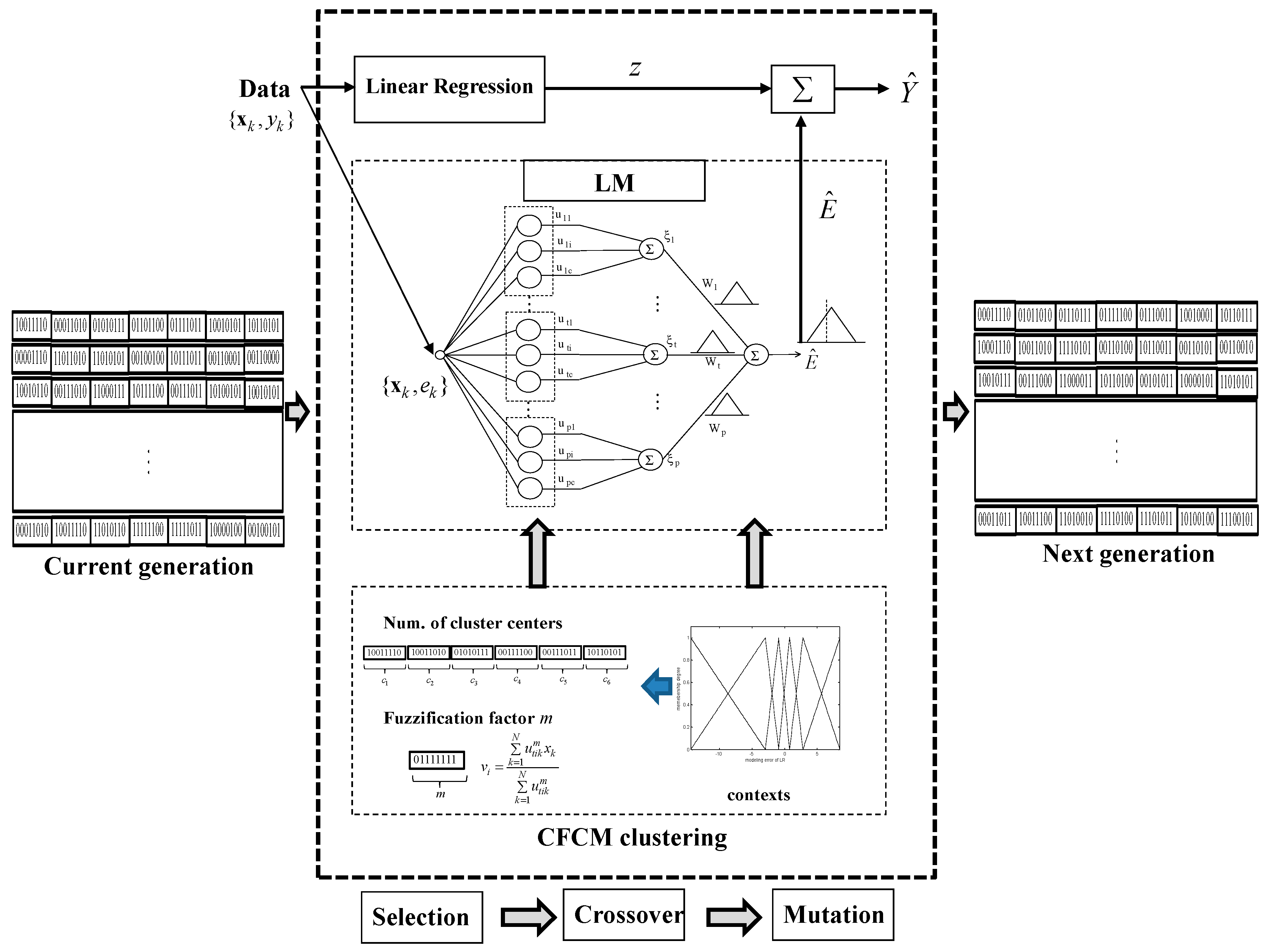
This paper is organized as follows. Section 2 gives an overview, architecture, and fundamental idea of the IGM. The IGM consists of several computing paradigms, including LR, CFCM clustering, and LM. Section 3 provides the optimization procedure and major components of the GA-based IGM. In Section 4, the experiments are performed on a coagulant dosing process in a water purification plant, automobile mpg (miles per gallon) prediction, and Boston housing data set, and results are discussed. Concluding comments are provided in Section 5.
2. Incremental Granular Model (IGM)
The IGM constituents consist of an LR as a global model, Context-based Fuzzy C-Means (CFCM) clustering [29], and a Linguistic Model (LM) [16] as a local model. Each of these constituent methodologies has its own strengths. The seamless integration of these methodologies forms the core of the IGM design.
2.1. Linear Regression (LR) as a Global Model
We suppose that the experimental data under discussion consists of two-dimensional input and output pairs for simplicity. These data points come in the form Here is the kth input vector and is the kth output. The LR model is given in the standard form as follows:
where the coefficients of the regression are denoted here by and . These coefficients are determined through the standard least-square error method, as encountered in statistics. Here is a vector with two coefficients . The enhancement of the model, for which the granular part comes into play, is based on the transformed data , where the residual part manifests through the expression , which denotes the error of the linear model. These data pairs are used to develop the incremental granular rule-based part of the model. Given the characteristics of the data, this rule-based model associates an input data point with the modeling error produced by the LR model. The rules and information granules are constructed using CFCM clustering.
2.2. CFCM Clustering with the Use of Information Granules
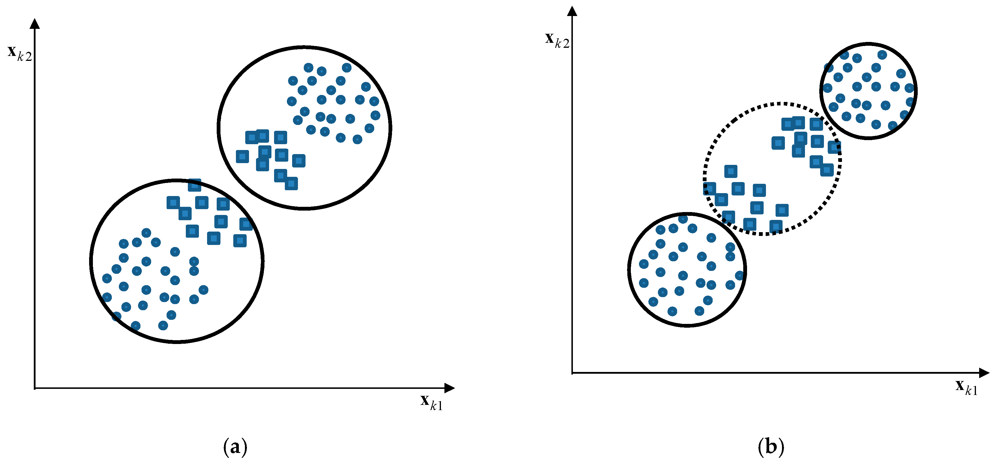
CFCM clustering [29] is an effective approach to estimating the cluster centers such that homogeneity is preserved, and is based on fuzzy granulation. To illustrate this clustering, let us briefly describe it for a simple training set as shown in Figure 1. The small circle and square of the data points reflect the corresponding values assumed by the dependent variable Figure 1a shows two evident clusters generated by the context-free fuzzy clustering algorithm. However, these clusters change when we reflect the corresponding output value. Figure 1b shows an extra cluster to preserve homogeneity with respect to the output variable. We can recognize from Figure 1 that the clusters obtained from CFCM clustering have better homogeneity than those produced by context-free fuzzy clustering.
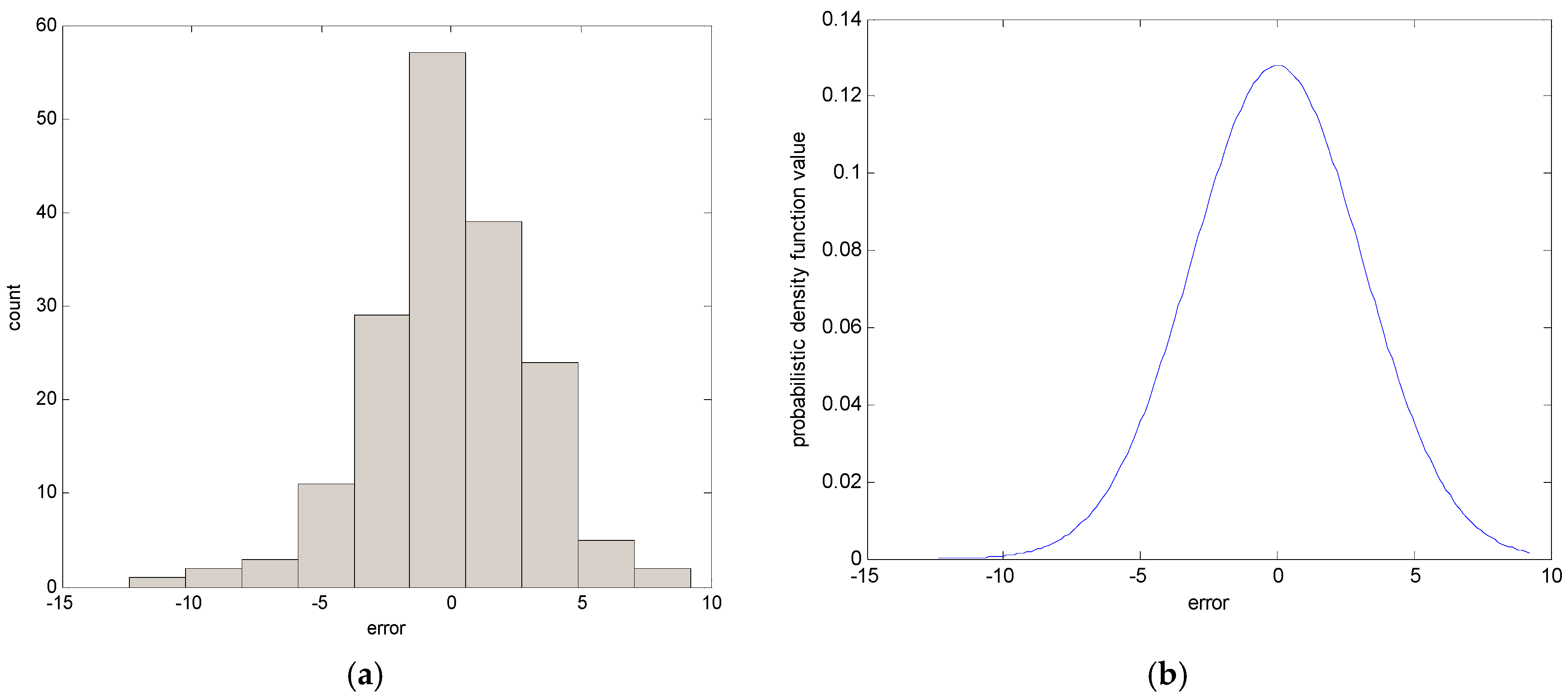
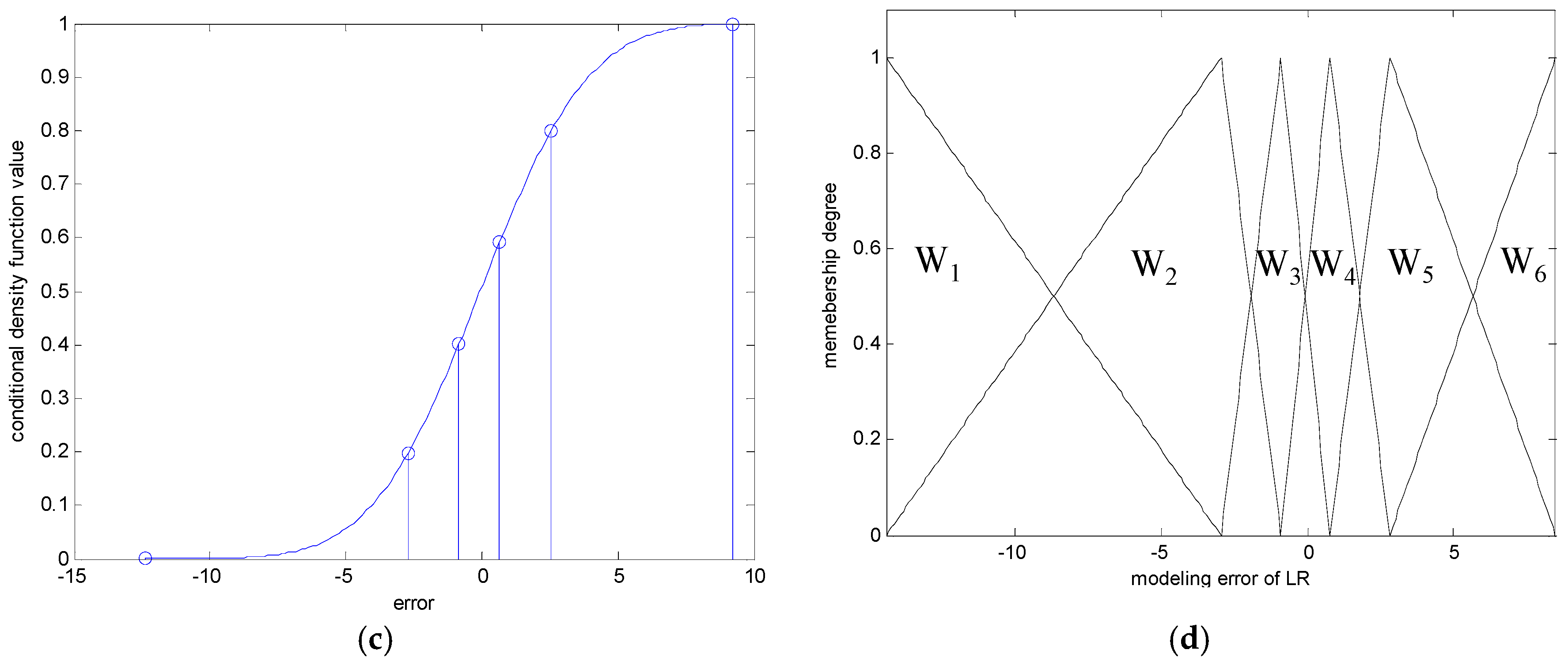
In the following, we briefly recall the essence of CFCM clustering. This clustering is realized for individual contexts by a statistical distribution in the output space. In the conventional LM as a granular model [16], these contexts are generated through a series of triangular fuzzy sets that are equally spaced along the domain of an output variable. However, it may be difficult to obtain the cluster centers in each context, because we may encounter a data scarcity problem resulting from scarce data being included in some contexts. Thus, this problem makes it difficult to obtain fuzzy rules from the CFCM clustering. Therefore, we use a probabilistic distribution for the output variables to produce flexible contexts. Figure 2 illustrates the automatic generation of linguistic contexts based on a histogram, probability density function, and conditional density function, in order [30,31]. First, we obtain a histogram from the error values. Second, we obtain a Gaussian distribution from the histogram, as shown in Figure 2b. Next, the accumulation of probabilities is performed. When p = 6, the centers of each context are located at the cumulative values [0 0.2 0.4 0.6 0.8 1], as shown in Figure 2c. Finally, the contexts with triangular fuzzy sets are generated in Figure 2d. Here, the obtained contexts are assigned a linguistic label, such as small error or large error. As shown in Figure 2, the x-axis is error obtained using the LR model mentioned in Section 2.1. These error values are used as the output data when CFCM clustering is performed.
Let us introduce the partition matrices induced by the tth context as follows [29]:
where denotes the membership degree of the kth data point and the tth context. Figure 3 shows the tth context and cluster centers obtained by .
In Equation (2), is the membership degree corresponding to kth data point and ith cluster center. The cost function can be expressed as follows:
where is the ith cluster center, and denotes the Euclidean distance between the kth input and the ith cluster center. The typical value of the weighting exponent m is set to 2. The minimization of the cost function is performed by updating the membership degrees of the partition matrix and the cluster centers corresponding to each context. The updating of the partition matrix is calculated as follows [29]:
where represents the element of the partition matrix by the ith cluster center and kth data point in the tth context. The cluster center is calculated in the form
This value yields a gradual transition between the rules and identifies smooth nonlinearities of the input–output relationships of the model. Thus, this value plays an important role in the system modeling because the characteristics of the model are represented differently for different values of the cluster centers. In this paper, the weighting exponent will be optimized using GA. The computations of the cluster centers are the same as for the original FCM clustering algorithm. Moreover, the convergence conditions for this method are the same as those discussed for the original FCM clustering algorithm [29]. Figure 4 shows a detailed view of the case of three contexts and two clusters per context.
2.3. Linguistic Model (LM) as a Local Model
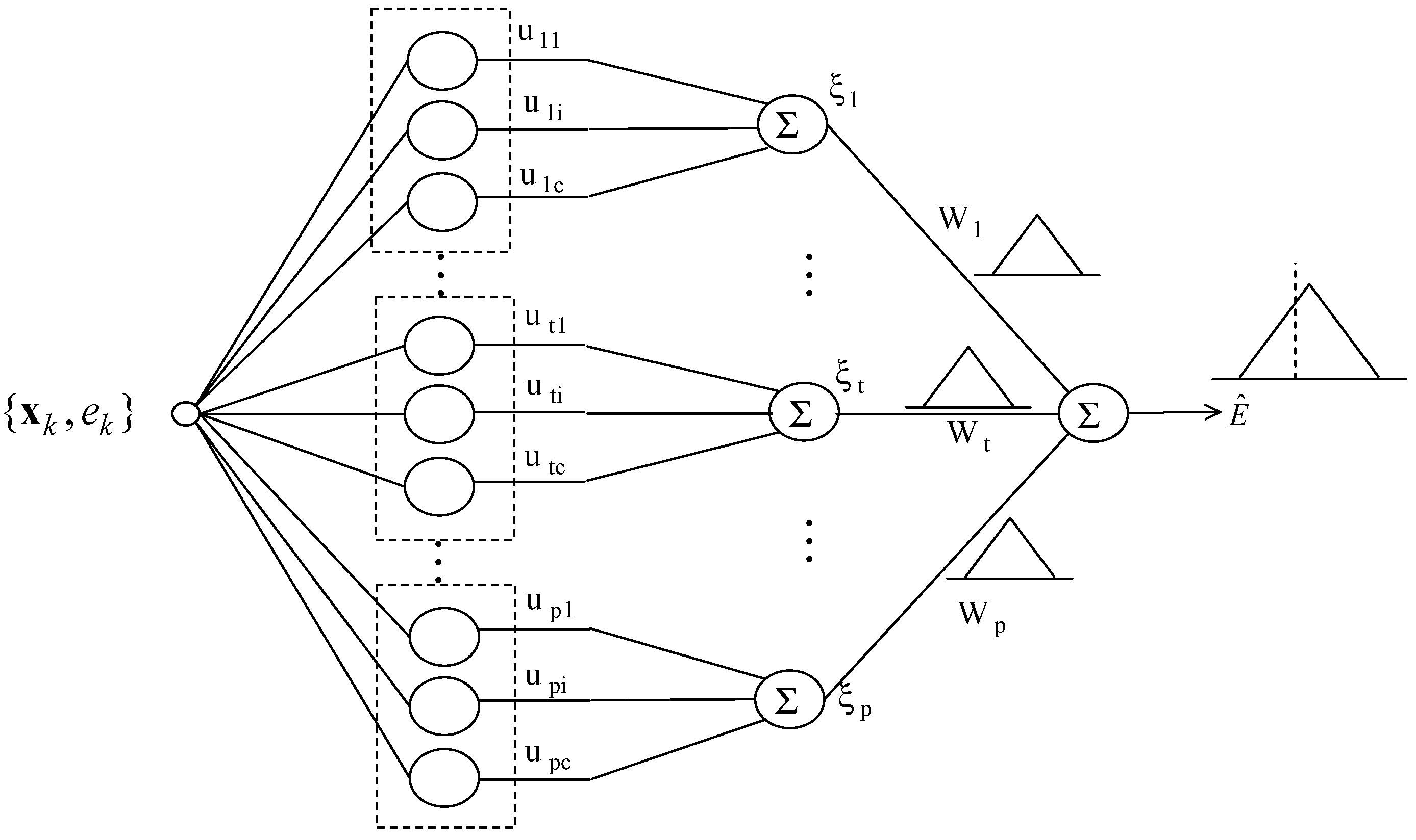
Figure 5 illustrates the architecture of the LM. As shown in Figure 5, the activation levels are afterwards summed up. The output of the LM represents the triangular fuzzy number showing a fuzzy set. That is, the model output is completely characterized by its three parameters, which are a modal value, the lower bound, and the upper bound .
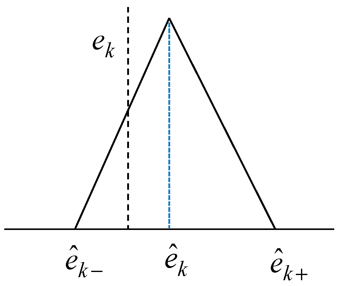
Figure 6 shows the triangular fuzzy number for the kth data point. Here, denotes the actual error for a given input . As shown in Figure 6, the predicted value is represented as triangular fuzzy number.
Assuming the triangular fuzzy sets for the contexts, a triangular fuzzy number is expressed as [16]
where the algebraic operations denoted by and are used to emphasize that the underlying computations operate on a collection of fuzzy numbers, and is the total sum of activation-level values produced at the kth context. The activation-level values in each context are calculated from Equation (4). We use the numeric bias term to eliminate possible systematic errors as follows:
where represents the modeling error obtained from LR as a global model. The numeric bias term could be obtained by augmenting the summation node. This term is computed in a straightforward manner, to eliminate potential systematic errors [16]. The resulting granular output admits the following characterization for its three parameters representing the lower bound, modal value, and upper bound:
2.4. Incremental Granular Model (IGM)
The fundamental scheme of the IGM design is illustrated in Figure 7. As shown in Figure 7, we perform the development of the Linear Regression (LR), followed by the construction of the local granular-based constructs that attempt to eliminate errors produced by the regression part of the model.
In the following, we recount the main design procedure for the IGM. The design procedure for the IGM is described in the following steps [27].
- [Step 1]
- Perform prediction using LR for the original input–output data pairs. Then, we obtain the modeling errors between the actual output and the model output of LR. From the original data set, a collection of input-error pairs is obtained.
- [Step 2]
- Generate the contexts in the error space. The contexts are obtained by the statistical characteristics of data distribution.
- [Step 3]
- Perform the CFCM clustering in the input space associated with the contexts generated in the error space. In the design of a conventional LM, we obtain clusters for contexts with clusters in each context. However, we need to determine the number of clusters that reflect the inherent characteristics of some input data pairs assigned from each context. Thus, we find the optimized number of cluster centers based on an evolutionary algorithm such as GA, described in the next section.
- [Step 4]
- Obtain the activation levels of the clusters produced by the corresponding contexts, and compute the overall aggregation by weighting through fuzzy sets of contexts. As a result, the IGM output yields a triangular fuzzy number, as shown in Figure 7.
- [Step 5]
- Combine the output of LR with the granular result of LM. Consequently, the final prediction is obtained as .
3. Genetically Optimized Incremental Granular Model
In this section, we present the optimization procedure based on a GA in the design of the IGM. Thus, we develop a genetically optimized IGM approach. As a result, the number of clusters in each context and the weighting exponent are optimized using a derivative-free stochastic optimization method, in contrast to using a fixed number of clusters in each context and adopting a typical weighting factor, as in the design of a conventional IGM.
The GA encodes each parameter to be optimized into a binary bit string, and each parameter is related with a fitness value that is equal to the objective function computed at that parameter. The GA is composed of a set of individuals as a population. Here, the population evolves towards a better fitness value. In each generation, the GA produces a new population using genetic operators, such as crossover and mutation. The GA approach used in this paper includes an encoding scheme, fitness evaluation, parent selection, a crossover operator, elitism scheme, and a mutation operator [21,22].
Based on the concepts mentioned above, the GA procedure in the design of IGM is described in the following steps:
- [Step 1]
- Initialize a population with randomly generated individuals, and set the crossover and mutation rates and bit number. In this paper, we adopt a bit number of eight, because we limit the number of clusters to between two and nine in each context.
- [Step 2]
- Evaluate the fitness value for each individual for the fitness function. The GA simultaneously performs a parallel search through the populations, with the number of different contexts ranging from five to eight. Thus, the number of parameters to be optimized varies for each population.
- [Step 3]
- Select two individuals from the population with probabilities proportional to the fitness values in each population. The coding scheme involves arranging the numbers of clusters generated by each context and the weighting factor into a chromosome, such that the representation preserves certain good properties after recombination, as specified by the crossover and mutation operators.
- [Step 4]
- Apply crossover and mutation with a certain probability for crossover and mutation rates, respectively.
- [Step 5]
- Repeat Steps 2 to 4 until a stopping criterion is met.
The evaluation of fitness function involves calculating the fitness value for each individual in the population after creating a generation. The fitness value of each individual is computed by the objective function for a maximization problem. The fitness function should quantitatively measure how fit a given solution is in solving the problem. Here we use a simple and effective fitness function frequently used in conjunction with GA, among various methods, as follows:
where and are the desired outputs for the training and testing data sets, respectively; and and are the model outputs for the training and testing data sets, respectively. Here, we use the standard root mean square error (RMSE) to express the matching level of the output of the IGM. The selection process determines which parents participate in producing offspring for the next generation.
In the encoding scheme, we transform the cluster number and the weighting exponent in the parameter space into bit string representations. Figure 8 shows a representation of the encoding scheme for the cluster number and weighting exponent when the bit number is 8. For example, in the case of , these parameters can be represented by a concatenated binary string. Here, each coordinate value is encoded as a gene composed of eight bits using binary coding. As shown in Figure 8, the last row represents the ranges of the number of clusters and the weighting exponent to be optimized, respectively.
The selection operation determines which parents participate in producing offspring for the next generation. The crossover process is applied to selected pairs of parents with a probability determined by a given crossover rate. In this study, we use the most basic one-point crossover operator. The crossover point is randomly selected, and two parent chromosomes are interchanged at this point. The mutation process changes the selected bit with a probability determined by a given mutation rate. Thus, it can prevent the population from converging to any local optima. Furthermore, we choose the elitism principle of always keeping a certain number of best members when each new population is generated. Figure 9 visualizes a schematic diagram illustrating how to produce the next generation from the current one in the design of the GA-based IGM. As shown in Figure 9, this process is performed on encoding schemes, fitness evaluations, parent selection, the crossover operator, and the mutation operator to produce the next generation.
4. Experimental Results
In this section, we describe comprehensive experiments that were performed, and draw conclusions. We shall demonstrate the performance of the GA in the optimization design of the IGM. For this purpose, we apply the proposed GA-based IGM to a coagulant dosing process in a water purification plant, automobile mpg prediction, and a Boston housing data set as real-world problems.
4.1. Coagulant Dosing Process in a Water Purification Plant
The field test data for this process was obtained at the AMSA water purification plant, Seoul, Korea, with a water purification capacity of 1,320,000 ton/day. We used 346 successive samples from jar-test data during one year. The input variables are composed of the turbidity of the raw water, temperature, pH, and alkalinity. The output variable is PAC (poly-aluminum chloride), widely used as a coagulant in water purification plants. We divided the data sets into training and checking data sets to evaluate the resultant model. In this experiment, we used 173 training data pairs for the model design of the GA-based IGM, while the remaining testing data sets were used for model evaluation.
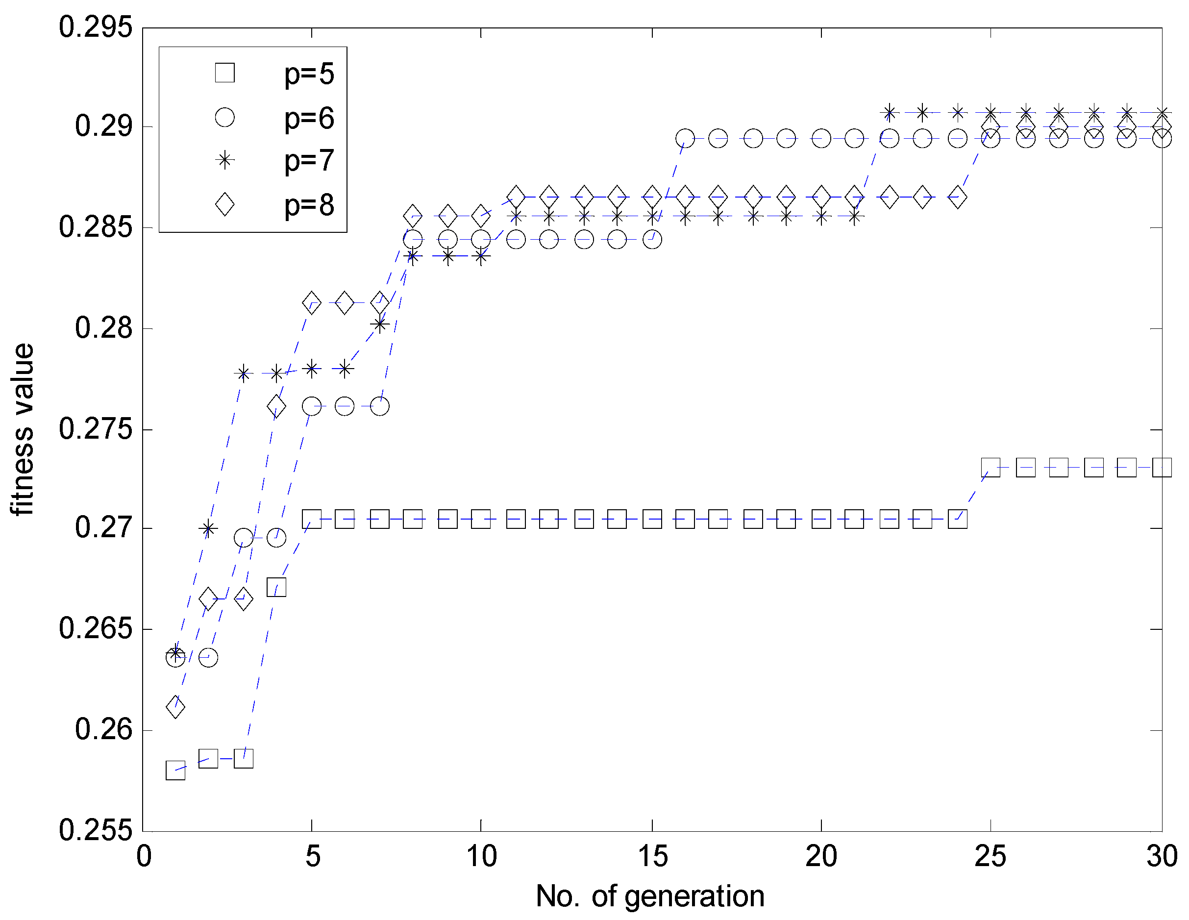
In order to optimize the parameters using the GA, we limit the search domain by setting the number of clusters to be between two and nine in each context and the weighting exponent to range from 1.5 to 3. Here, we adopt a new optimization strategy, because the number of chromosomes differs from the number of contexts. Thus, we perform parallel GA through four groups (populations) of LM, with the number of different contexts ranging from five to eight. We used eight-bit binary coding for each parameter of the cluster number and the weighting exponent. Each generation in the GA implementation contains 30 individuals. Moreover, we used a simple one-point crossover scheme, with the crossover rate equal to 0.97, and uniform mutation with the mutation rate equal to 0.01. We also applied elitism to keep the best two individuals across generations.
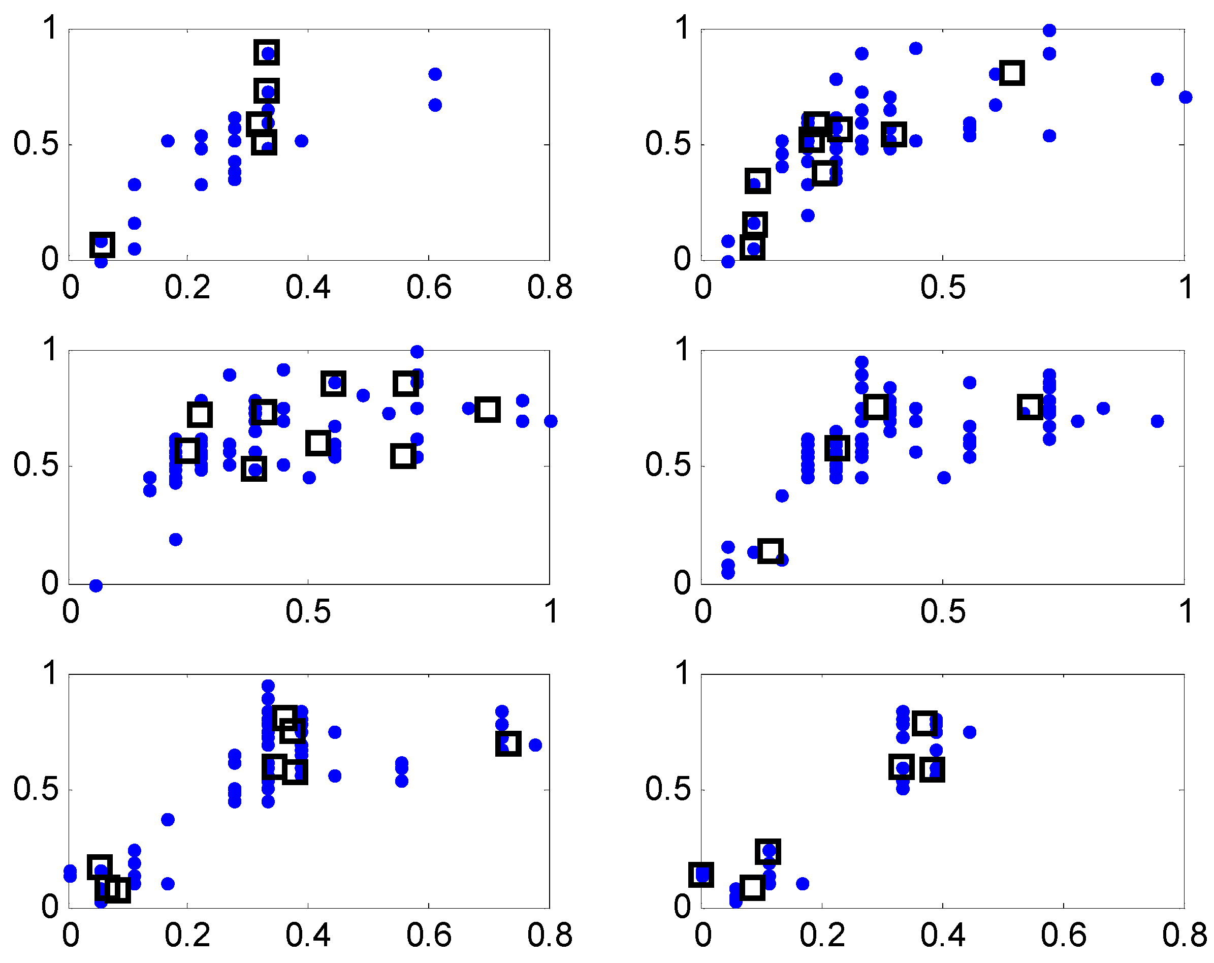
Figure 10 shows the contexts obtained from the error space when the number of contexts is from five to eight. Here, the error values are residuals obtained from the LR model. Figure 11 illustrates the distribution of data and cluster centers generated in six contexts after performing GA. These clusters build information granules in the form of fuzzy sets, and are used to produce fuzzy if-then rules. Figure 12 illustrates the performance of parallel GA across generations. Here, we finally obtained the best parameters (number of clusters: c = [3, 9, 4, 5, 9, 7, 6], weighting exponent: m = 1.9285) when the number of linguistic contexts is seven (p = 7). As shown in Figure 12, we determine the best case of the fitness value across 30 generations when the number of contexts varies from five to eight. In order to obtain the best model, we used the elitism scheme so that the solution quality obtained by the GA will not decrease from one generation to the next. The best curve is monotonically increasing with respect to the generation numbers, because we used elitism scheme to keep the best two individuals from each generation. Table 1 lists the parameters optimized by the GA for the coagulant dosing process example.
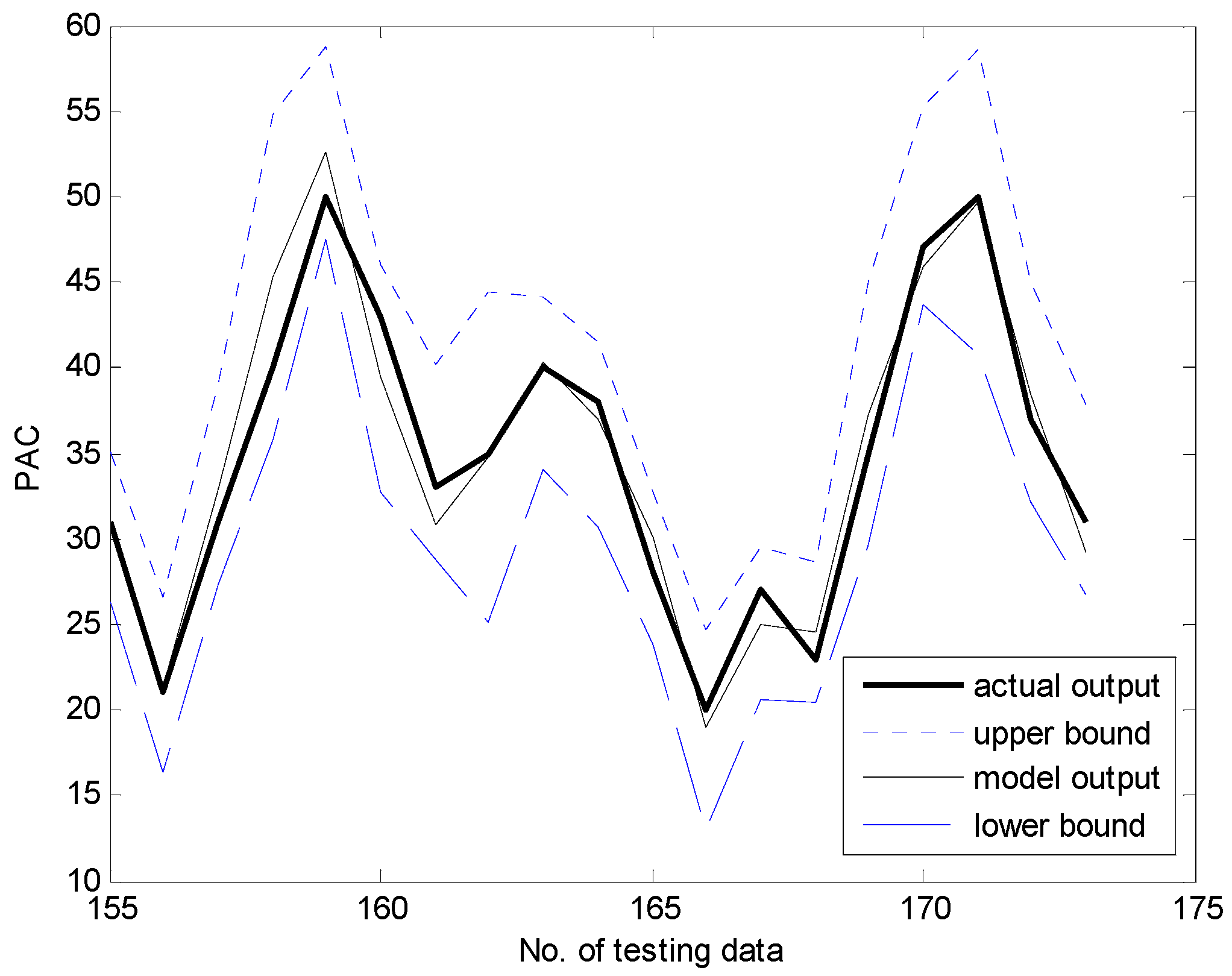
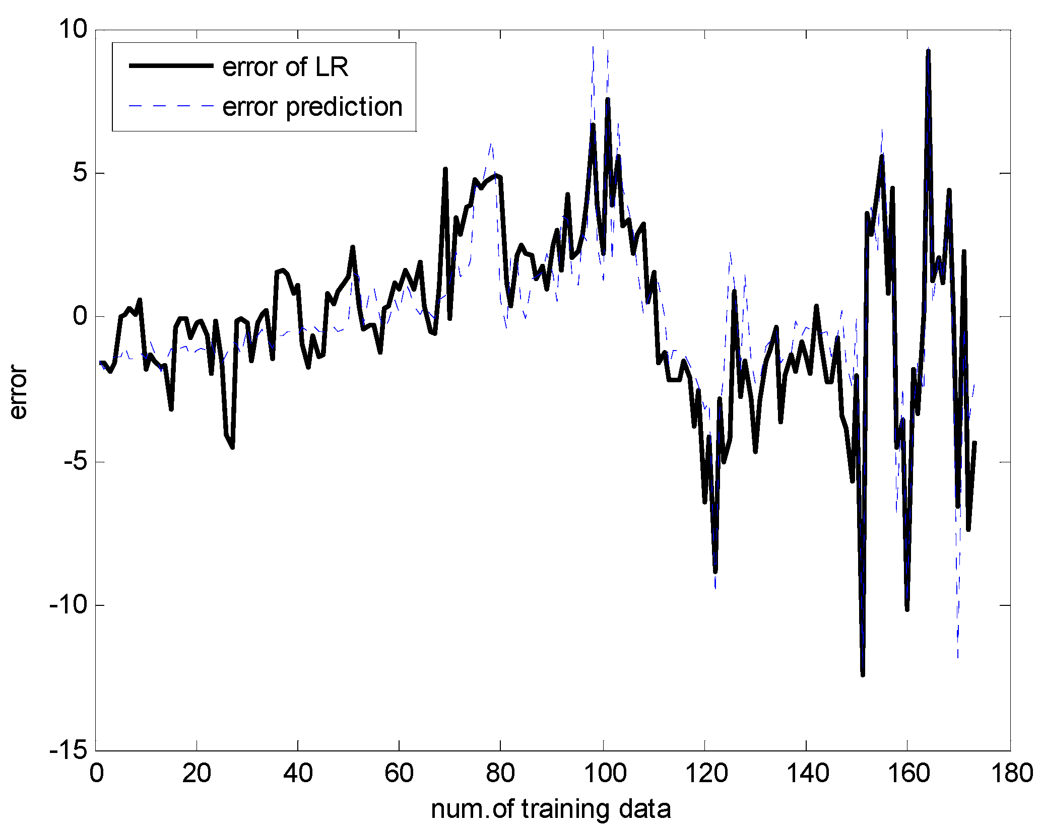
Figure 13 and Figure 14 present a comparison between the desired and model output for the training data and checking data, respectively. As shown in these figures, it is obvious that the proposed GA-based IGM approach achieved good approximation and generalization performance. In particular, it can be seen that the output data with strong nonlinearity is well predicted. Figure 15 illustrates the interval prediction performance represented by the lower bound, modal output, and upper bound for part of the testing data set. The interval prediction is generated by a triangular fuzzy number from the LM, forming a specific model output. Figure 16 shows the error prediction obtained from the local LM. In particular, it was found that the data with large errors was well predicted. As a result, the error prediction can compensate the residuals obtained from LR as a first-principle global model. Table 2 lists the comparison results of the RMSE for the training and testing data for the coagulant dosing process. These experiments were performed in the computer environment of and Intel Core i7-4790 CPU with MATLAB R2015A. The processing time of the IGM is 0.06 s (p = c = 6), while the average processing time of the proposed GA-based IGM is 2.06 s for one generation. In the case of 30 generations, the processing time of the GA-based IGM is 69.91 s. On the other hand, the processing time of the LM is 0.09 s (p = c = 6), while the average processing time of the proposed GA-based LM is 5.1 s for one generation. In the case of 30 generations, the processing time of GA-based LM is 153.04 s. As listed in Table 2, the experimental results revealed that the proposed GA-based IGM achieved good performance in comparison with previous methods such as LR, MLP, CFCM-RBFNN, LM, GA-based LM, and IGM itself. Here the proposed GA-based IGM achieved the best performance in terms of the generalization capability when the number of contexts and fuzzy rules are 7 and 43, respectively. The GA-based IGM obviously outperformed the conventional IGM. Moreover, it was found from the results that the GA-based IGM obtained the optimal fuzzy if-then rules and weighting exponent, in contrast to the method by trial and error.
4.2. Automobile mpg Prediction and Boston Housing Data Sets
The automobile mpg prediction data and Boston housing data sets are available from the UCI repository of machine learning databases [32]. First, we shall use the automobile mpg prediction. After removing instances with missing values, the data set was reduced to 392 data pairs. The input attributes consists of weight, acceleration, model year, cylinder number, displacement, and horsepower [18,19]. We divided the data set into training and testing data sets. In this experiment, we used 196 training data pairs for the model design of the GA-based IGM, while the remaining testing data sets were used for model evaluation. Table 3 lists the parameters optimized by GA for automobile mpg prediction. Table 4 lists the comparison results of the RMSE for the training and testing data for the automobile mpg prediction. As listed in Table 4, we finally obtained the best parameters (number of clusters: c = [6, 5, 8, 5, 9, 8, 8, 9], number of rules: 58, weighting exponent: m = 1.9285) when the number of linguistic contexts is seven (p = 8). The experimental results revealed that the proposed GA-based IGM achieved good performance in comparison with previous methods such as IGM itself.
Next, we shall use the Boston housing data set that deals with the problem of real estate price prediction. In this example, we used twelve input variables except for one binary attribute. The total data includes 506 data pairs. We divided the data set into training and testing data sets of equal size. In this study, we used 253 training data pairs for the model design of the GA-based IGM, while the remaining testing data sets were used for model evaluation. Table 5 lists the parameters optimized by GA for the Boston housing data. Table 6 lists the comparison results of the RMSE for the training and testing data for Boston housing data. As listed in Table 6, we finally obtained the best parameters (number of clusters: c = [4, 8, 9, 9, 5, 9, 2], number of rules: 46, weighting exponent: m = 1.5) when the number of linguistic contexts is seven (p = 7). The experimental results clearly showed that the proposed method was superior to the IGM.
5. Conclusions
We developed a design methodology using a genetically oriented rule-based IGM with the aid of information granulation. For this, we used parallel GA, which is a derivative-free stochastic optimization method based on the concepts of natural selection and evolutionary processes. Thus, we optimized the number of clusters and rules obtained from each context and the weighting exponent. To evaluate the performance of the proposed method, we applied it to a coagulant dosing process in a water purification plant, automobile mpg prediction, and Boston housing data as real-world application problems. The experimental results revealed that the GA-based IGM achieved a good performance in comparison with previous models. For further research, we will evaluate the quantifying performance of granular fuzzy models representing coverage and specificity characteristics. In addition, we will simultaneously optimize several parameters of the IGM using particle swarm optimization [33,34,35].
Author Contributions
Yeong-Hyeon Byeon suggested the idea for this work and performed the experiments. Keun-Chang Kwak designed the experimental method. Both authors wrote and critically revised the paper.
Conflicts of Interest
The authors declare no conflict of interest.
References
- Jang, J.S.R.; Sun, C.T.; Mizutani, E. Neuro-Fuzzy and Soft Computing: A Computational Approach to Learning and Machine Intelligence; Prentice Hall: Upper Saddle River, NJ, USA, 1997. [Google Scholar]
- Pedrycz, W.; Gomide, F. Fuzzy Systems Engineering: Toward Human-Centric Computing; IEEE Press: New York, NY, USA, 2007. [Google Scholar]
- Miranian, A.; Abdollahzade, M. Developing a local least-squares support vector machines-based neuro-fuzzy model for nonlinear and chaotic time series prediction. IEEE Trans. Neural Netw. Learn. Syst. 2013, 24, 207–218. [Google Scholar] [CrossRef] [PubMed]
- Li, W.; Hu, X.; Gravina, R.; Fortino, G. A neuro-fuzzy fatigue-tracking and classification system for wheelchair users. IEEE Access 2017, 5, 19420–19431. [Google Scholar] [CrossRef]
- Tsai, J.T.; Chou, J.H.; Lin, C.F. Designing micro-structure parameters for backlight modules by using improved adaptive neuro-fuzzy inference system. IEEE Access 2015, 3, 2626–2636. [Google Scholar] [CrossRef]
- Siminski, K. Interval type-2 neuro-fuzzy system with implication-based inference mechanism. Expert Syst. Appl. 2017, 79, 140–152. [Google Scholar] [CrossRef]
- Shvetcov, A. Models of neuro-fuzzy agents in intelligent environments. Procedia Comput. Sci. 2017, 103, 135–141. [Google Scholar] [CrossRef]
- Jelusic, P.; Zlender, B. Discrete optimization with fuzzy constraints. Symmetry 2017, 9, 87. [Google Scholar] [CrossRef]
- Ramos, G.A.R.; Akanji, L. Data analysis and neuro-fuzzy technique for EOR screening: Application in Angolan oilfields. Energies 2017, 10. [Google Scholar] [CrossRef]
- Chen, W.; Panahi, M.; Pourghasemi, H.R. Performance evaluation of GIS-based new ensemble data mining techniques of adaptive neuro-fuzzy inference system (ANFIS) with genetic algorithm (GA), differential evolution (DE), and particle swarm optimization (PSO) for landslide spatial modeling. CATENA 2017, 157, 310–324. [Google Scholar] [CrossRef]
- Shihabudheen, K.V.; Pillai, G.N. Regularized extreme learning adaptive neuro-fuzzy algorithm for regression and classification. Knowl.-Based Syst. 2017, 127, 100–113. [Google Scholar]
- Kumaresan, N.; Ratnavelu, K. Optimal control for stochastic linear quadratic singular neuro Takagi-Sugeno fuzzy system with singular cost using genetic programming. Appl. Soft Comput. 2014, 24, 1136–1144. [Google Scholar] [CrossRef]
- Lin, C.J. An efficient immune-based symbiotic particle swarm optimization learning algorithm for TSK-type neuro-fuzzy networks design. Fuzzy Sets Syst. 2008, 159, 2890–2909. [Google Scholar] [CrossRef]
- Oh, S.K.; Kim, W.D.; Pedrycz, W.; Park, B.J. Polynomial-based radial basis function neural networks (P-RBF NNs) realized with the aid of particle swarm optimization. Fuzzy Sets Syst. 2011, 163, 54–77. [Google Scholar] [CrossRef]
- Pedrycz, W. Conditional fuzzy clustering in the design of radial basis function neural networks. IEEE Trans. Neural Netw. 1998, 9, 601–612. [Google Scholar] [CrossRef] [PubMed]
- Pedrycz, W.; Kwak, K.C. Linguistic models as a framework of user-centric system modeling. IEEE Trans. Syst. Man Cybern. Part A Syst. Hum. 2006, 36, 727–745. [Google Scholar] [CrossRef]
- Pedrycz, W. A dynamic data granulation through adjustable fuzzy clustering. Pattern Recognit. Lett. 2008, 29, 2059–2066. [Google Scholar] [CrossRef]
- Chalmers, E.; Pedrycz, W.; Lou, E. Human experts’ and a fuzzy model’s predictions of outcomes of scoliosis treatment: A comparative analysis. IEEE Trans. Biomed. Eng. 2015, 62, 1001–1007. [Google Scholar] [CrossRef] [PubMed]
- Reyes-Galaviz, O.F.; Pedrycz, W. Granular fuzzy models: Analysis, design, and evaluation. Int. J. Approx. Reason. 2015, 64, 1–19. [Google Scholar] [CrossRef]
- Kim, E.H.; Oh, S.K.; Pedrycz, W. Reinforced rule-based fuzzy models: Design and analysis. Knowl.-Based Syst. 2017, 119, 44–58. [Google Scholar] [CrossRef]
- Kwak, K.C.; Pedrycz, W. A design of genetically oriented linguistic model with the aid of fuzzy granulation. In Proceedings of the 2010 IEEE World Congress on Computational Intelligence, Barcelona, Spain, 18–23 July 2010. [Google Scholar]
- Kwak, K.C. A design of genetically optimized linguistic models. IEICE Trans. Inf. Syst. 2012, E95D, 3117–3120. [Google Scholar] [CrossRef]
- Climino, M.G.C.A.; Lazzerini, B.; Marcelloni, F.; Pedrycz, W. Genetic interval neural networks for granular data regression. Inf. Sci. 2014, 257, 313–330. [Google Scholar] [CrossRef]
- Oh, S.K.; Kim, W.D.; Pedrycz, W.; Seo, K. Fuzzy radial basis function neural networks with information granulation and its parallel genetic optimization. Fuzzy Syst. 2014, 237, 96–117. [Google Scholar] [CrossRef]
- Pedrycz, W.; Song, M. A genetic reduction of feature space in the design of fuzzy models. Appl. Soft Comput. 2012, 12, 2801–2816. [Google Scholar] [CrossRef]
- Hu, X.; Pedrycz, W.; Wang, X. Development of granular models through the design of a granular output spaces. Knowl.-Based Syst. 2017, 134, 159–171. [Google Scholar] [CrossRef]
- Pedrycz, W.; Kwak, K.C. The development of incremental models. IEEE Trans. Fuzzy Syst. 2007, 15, 507–518. [Google Scholar] [CrossRef]
- Li, J.; Pedrycz, W.; Wang, X. A rule-based development of incremental models. Int. J. Approx. Reason. 2015, 64, 20–38. [Google Scholar] [CrossRef]
- Pedrycz, W. Conditional fuzzy c-mans. Pattern Recognit. Lett. 1996, 17, 625–631. [Google Scholar] [CrossRef]
- Kwak, K.C.; Kim, D.H. TSK-based linguistic fuzzy model with uncertain model output. IEICE Trans. Inf. Syst. 2006, E89D, 2919–2923. [Google Scholar] [CrossRef]
- Kwak, K.C.; Kim, S.S. Development of quantum-based adaptive neuro-fuzzy networks. IEEE Trans. Syst. Man Cybern. Part B 2010, 40, 91–100. [Google Scholar]
- UCI Machine Learning Repository. Available online: https://archive.ics.uci.edu/ml/datasets (accessed on 26 November 2017).
- Zhu, X.; Pedrycz, W.; Li, Z. Granular encoders and decoders: A study in processing information granules. IEEE Trans. Fuzzy Syst. 2017, 25, 1115–1126. [Google Scholar] [CrossRef]
- Huang, W.; Oh, S.K.; Pedrycz, W. Fuzzy wavelet polynomial neural networks: Analysis and design. IEEE Trans. Fuzzy Syst. 2017, 25, 1329–1341. [Google Scholar] [CrossRef]
- Ding, Y.; Cheng, L.; Pedrycz, W.; Hao, K. Global nonlinear kernel prediction for large data set with a particle swarm-optimized interval support vector regression. IEEE Trans. Neural Netw. Learn. Syst. 2015, 26, 2521–2534. [Google Scholar] [CrossRef] [PubMed]
Figure 1.
Clusters generated by context-free and context-based clustering: (a) context-free clustering; (b) context-based clustering.
Figure 1.
Clusters generated by context-free and context-based clustering: (a) context-free clustering; (b) context-based clustering.

Figure 2.
Generation of contexts by statistical distribution of data: (a) histogram; (b) probability density function; (c) conditional density function; (d) contexts.
Figure 2.
Generation of contexts by statistical distribution of data: (a) histogram; (b) probability density function; (c) conditional density function; (d) contexts.


Figure 3.
Distribution of data and cluster centers corresponding to the tth context .
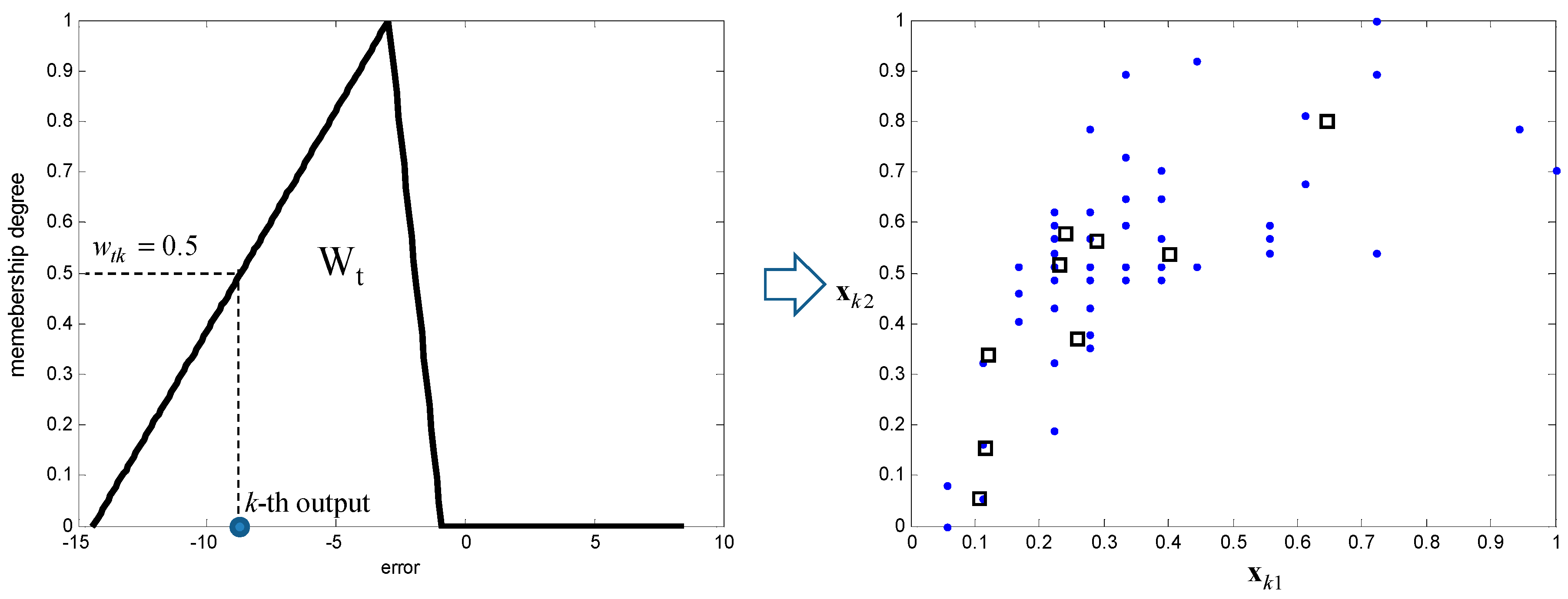
Figure 4.
Detailed view of the case of three contexts and two clusters per context.
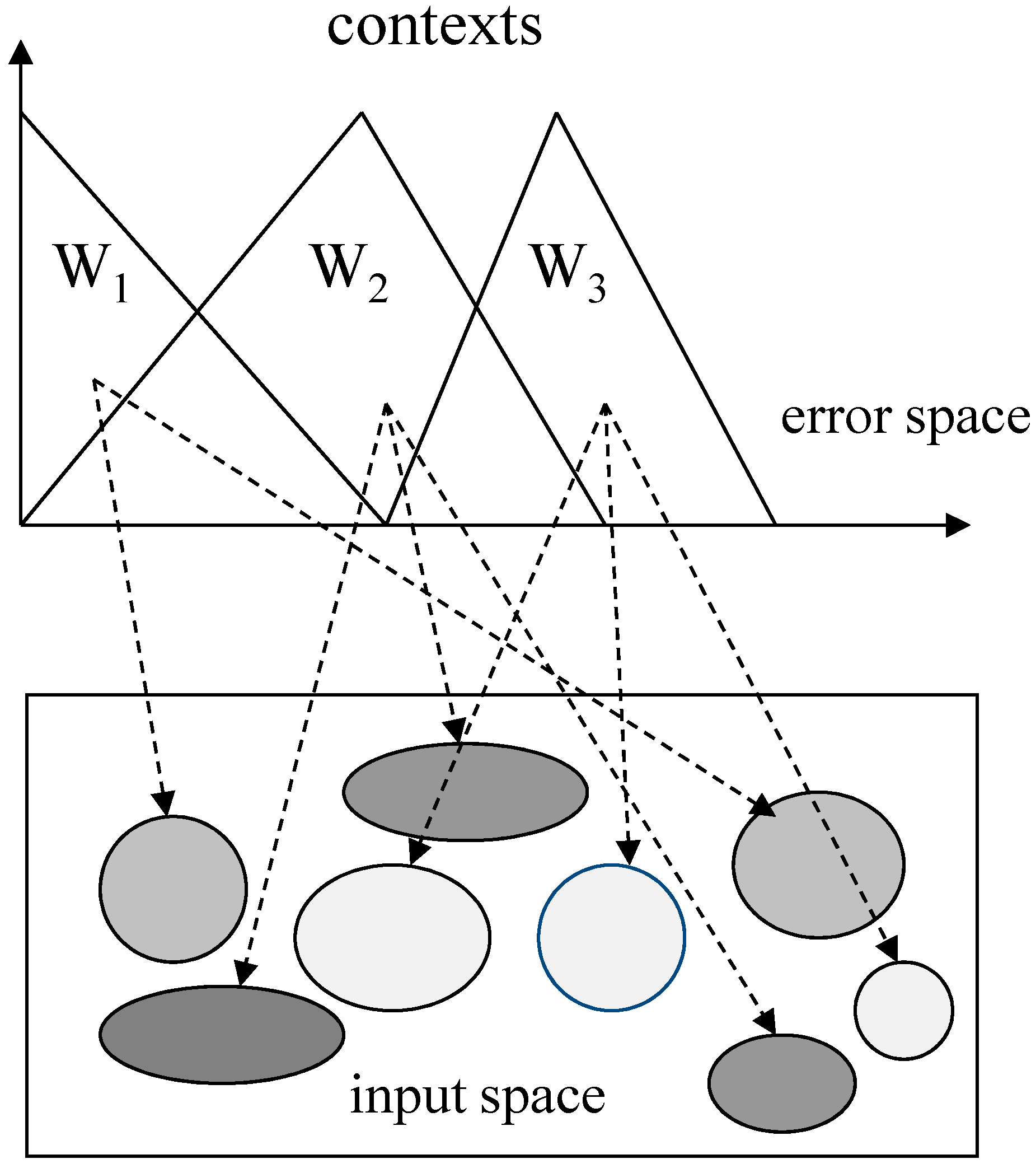
Figure 5.
Architecture of local Linguistic Model (LM).

Figure 6.
Actual error and the predicted fuzzy number .

Figure 7.
Architecture of the Incremental Granular Model (IGM). CFCM: Context-based Fuzzy C-Means.
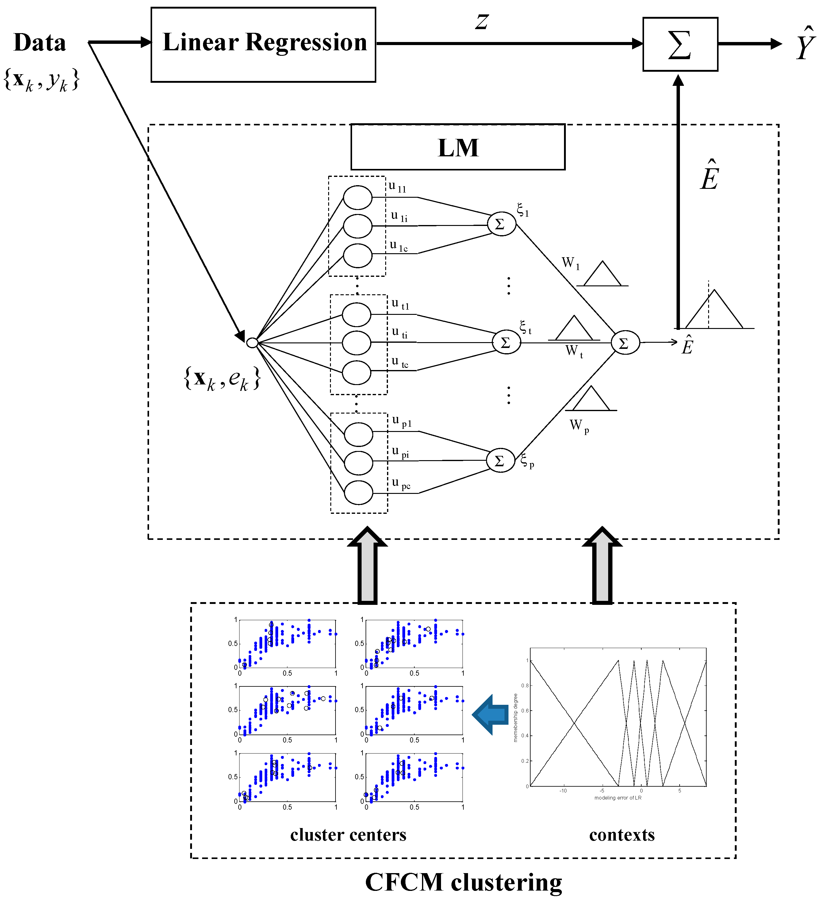
Figure 8.
Representation of encoding scheme (p = 6).
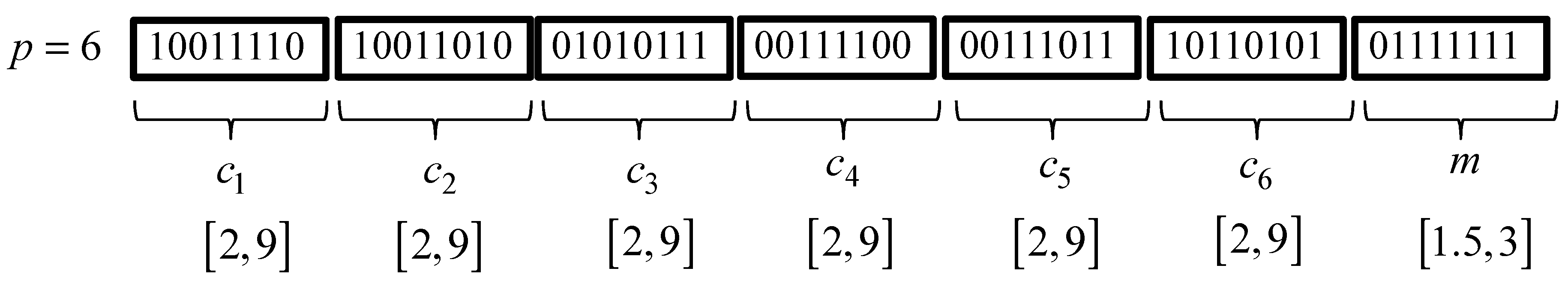
Figure 9.
Producing the next generation in the design of the Genetic Algorithms (GA)-based IGM.

Figure 10.
Contexts generated from the output space (x-axis: error). (a) p = 5; (b) p = 6; (c) p = 7; (d) p = 8.
Figure 10.
Contexts generated from the output space (x-axis: error). (a) p = 5; (b) p = 6; (c) p = 7; (d) p = 8.
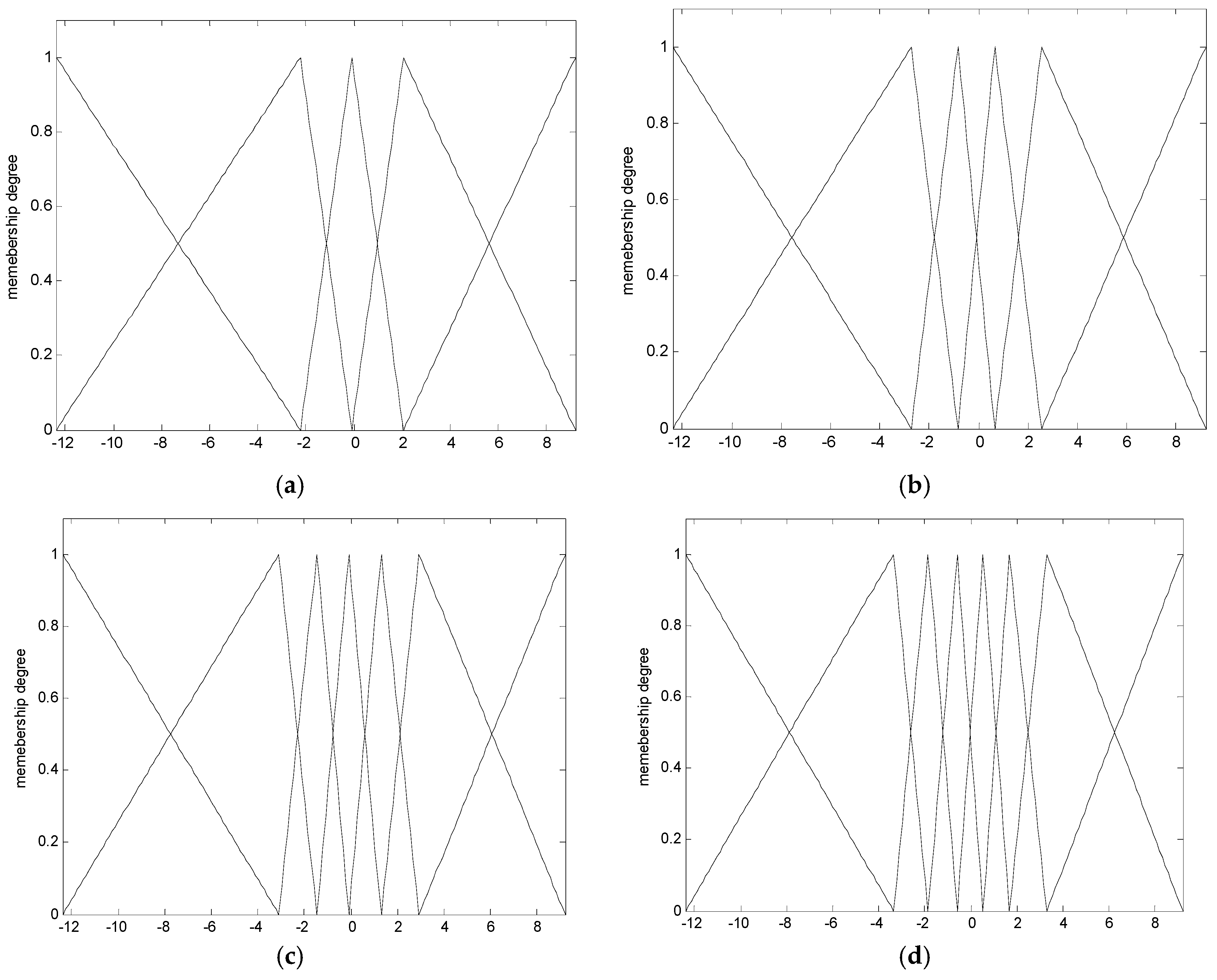
Figure 11.
Distribution of data and cluster center corresponding to six contexts (x-axis: y-axis: ).
Figure 11.
Distribution of data and cluster center corresponding to six contexts (x-axis: y-axis: ).

Figure 12.
Variation of fitness values by generation.

Figure 13.
Approximation capability for training data.
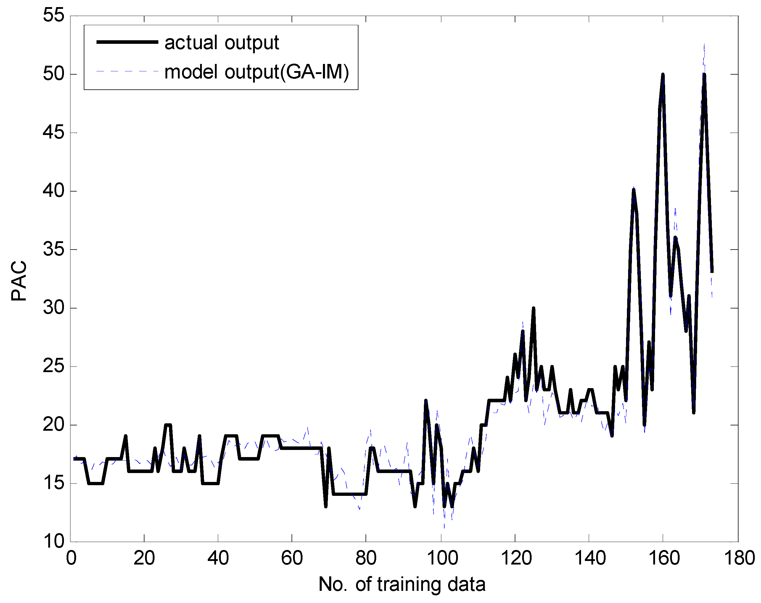
Figure 14.
Generalization capability for testing data.
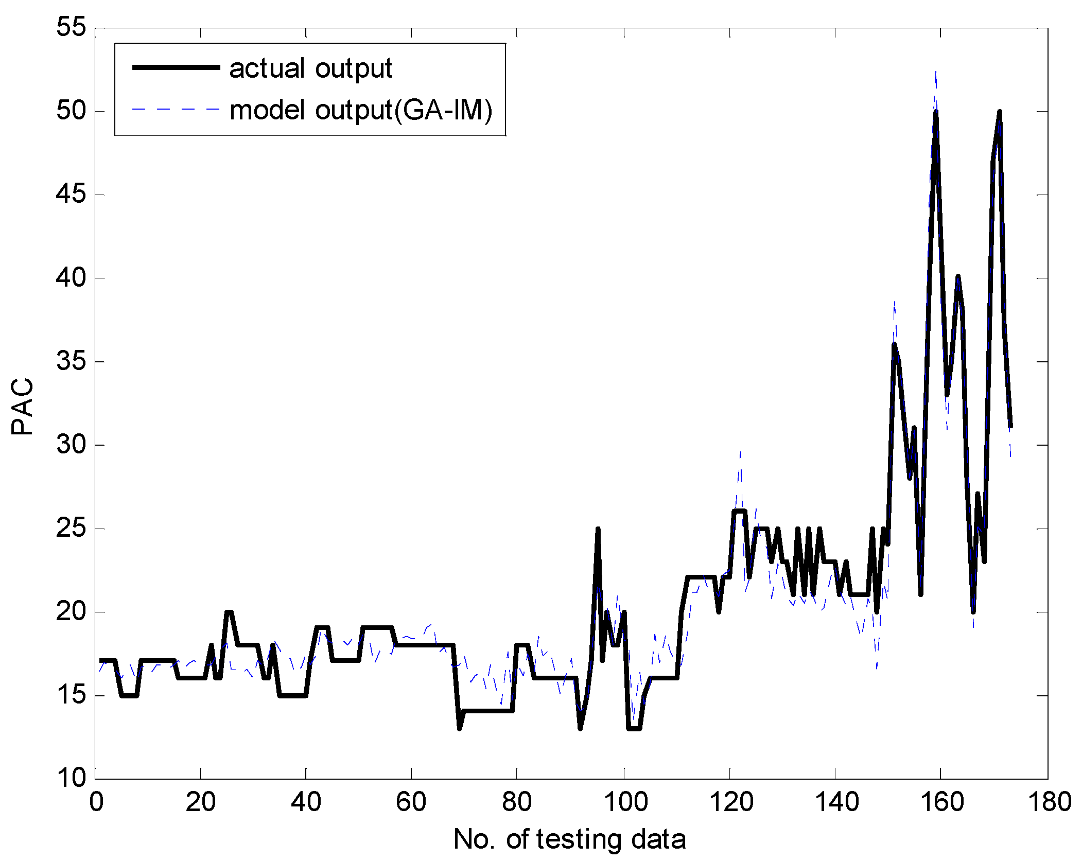
Figure 15.
Output of the GA-based IGM with interval prediction.

Figure 16.
Error values predicted by IGM as a local granular model.


Table 1.
Parameters optimized by the GA for the coagulant dosing process.
| p | No. of Cluster Center in Each Context | No. of Rule | Weighting Exponent |
|---|---|---|---|
| 5 | [5, 9, 2, 9, 7] | 32 | 2.1428 |
| 6 | [5, 9, 9, 4, 8, 6] | 41 | 1.9285 |
| 7 | [3, 9, 4, 5, 9, 7, 6] | 43 | 1.9285 |
| 8 | [3, 9, 8, 9, 7, 8, 9, 8] | 61 | 1.9285 |
Table 2.
Comparison results for RMSE (*: no. of nodes) for the coagulant dosing process. MLP: Multilayer Perceptron. RBFNN: Radial Basis Function Neural Network. TSK-LFM: Takagi-Sugeno-Kang-Linguistic Fuzzy Model.
Table 2.
Comparison results for RMSE (*: no. of nodes) for the coagulant dosing process. MLP: Multilayer Perceptron. RBFNN: Radial Basis Function Neural Network. TSK-LFM: Takagi-Sugeno-Kang-Linguistic Fuzzy Model.
| Method | No. of Rule | RMSE (Training) | RMSE (Testing) | |
|---|---|---|---|---|
| LR | - | 3.508 | 3.578 | |
| MLP | 45 * | 3.191 | 3.251 | |
| CFCM-RBFNN [15] | 45 * | 3.048 | 3.219 | |
| LM [16] (p = 8) | c = 6 | 48 | 2.549 | 2.820 |
| c = 7 | 56 | 2.526 | 2.835 | |
| c = 8 | 64 | 2.427 | 2.800 | |
| TSK-LFM [29] | 45 | 2.514 | 2.661 | |
| GA-based LM [22] | 47 | 2.060 | 2.290 | |
| IGM [27,28] | p = c = 6 | 36 | 2.228 | 2.364 |
| p = c = 7 | 49 | 1.971 | 2.117 | |
| p = c = 8 | 64 | 1.790 | 2.009 | |
| p = c = 9 | 81 | 1.855 | 2.084 | |
| GA-based IGM | p = 5 | 32 | 1.712 | 1.949 |
| p = 6 | 41 | 1.567 | 1.915 | |
| p = 7 | 43 | 1.607 | 1.832 | |
| p = 8 | 61 | 1.597 | 1.850 | |
Table 3.
Parameters optimized by GA for automobile mpg prediction.
| p | No. of Cluster Center in Each Context | No. of Rule | Weighting Exponent |
|---|---|---|---|
| 5 | [5, 6, 2, 9, 8] | 30 | 2.5714 |
| 6 | [5, 7, 8, 4, 9, 9] | 42 | 2.3571 |
| 7 | [5, 8, 9, 6, 5, 8, 9] | 50 | 2.1428 |
| 8 | [6, 5, 8, 5, 9, 8, 8, 9] | 58 | 1.9285 |
Table 4.
Comparison results for RMSE for automobile mpg prediction.
| Method | No. of Rule | RMSE (Training) | RMSE (Testing) | |
|---|---|---|---|---|
| LM [16] | 36 | 2.788 | 3.337 | |
| GA-based LM [22] | 52 | 2.328 | 3.120 | |
| IGM [27,28] | 36 | 2.418 | 3.175 | |
| GA-based IGM | p = 5 | 30 | 2.231 | 3.050 |
| p = 6 | 42 | 2.183 | 2.989 | |
| p = 7 | 50 | 2.108 | 2.964 | |
| p = 8 | 58 | 2.058 | 2.932 | |
Table 5.
Parameters optimized by GA for the Boston housing data set.
| p | No. of Cluster Center in Each Context | No. of Rule | Weighting Exponent |
|---|---|---|---|
| 5 | [7, 8, 2, 9, 2] | 28 | 1.9285 |
| 6 | [9, 9, 4, 5, 9, 7] | 43 | 1.9285 |
| 7 | [4, 8, 9, 9, 5, 9, 2] | 46 | 1.5000 |
| 8 | [6, 8, 8, 2, 4, 7, 9, 3] | 47 | 1.7142 |
© 2017 by the authors. Licensee MDPI, Basel, Switzerland. This article is an open access article distributed under the terms and conditions of the Creative Commons Attribution (CC BY) license (http://creativecommons.org/licenses/by/4.0/).
Share and Cite
MDPI and ACS Style
Byeon, Y.-H.; Kwak, K.-C. A Design for Genetically Oriented Rules-Based Incremental Granular Models and Its Application. Symmetry 2017, 9, 324. https://doi.org/10.3390/sym9120324
AMA Style
Byeon Y-H, Kwak K-C. A Design for Genetically Oriented Rules-Based Incremental Granular Models and Its Application. Symmetry. 2017; 9(12):324. https://doi.org/10.3390/sym9120324
Chicago/Turabian StyleByeon, Yeong-Hyeon, and Keun-Chang Kwak. 2017. "A Design for Genetically Oriented Rules-Based Incremental Granular Models and Its Application" Symmetry 9, no. 12: 324. https://doi.org/10.3390/sym9120324
Note that from the first issue of 2016, this journal uses article numbers instead of page numbers. See further details here.