Visualization of Thomas–Wigner Rotations


GFZ German Research Centre for Geosciences, Telegrafenberg, 14473 Potsdam, Germany
Symmetry 2017, 9(12), 292; https://doi.org/10.3390/sym9120292
Submission received: 1 November 2017
/
Revised: 7 November 2017
/
Accepted: 8 November 2017
/
Published: 27 November 2017
Abstract
:It is well known that a sequence of two non-collinear Lorentz boosts (pure Lorentz transformations) does not correspond to a Lorentz boost, but involves a spatial rotation, the Wigner or Thomas–Wigner rotation. We visualize the interrelation between this rotation and the relativity of distant simultaneity by moving a Born-rigid object on a closed trajectory in several steps of uniform proper acceleration. Born-rigidity implies that the stern of the boosted object accelerates faster than its bow. It is shown that at least five boost steps are required to return the object’s center to its starting position, if in each step the center is assumed to accelerate uniformly and for the same proper time duration. With these assumptions, the Thomas–Wigner rotation angle depends on a single parameter only. Furthermore, it is illustrated that accelerated motion implies the formation of a “frame boundary”. The boundaries associated with the five boosts constitute a natural barrier and ensure the object’s finite size.
1. Introduction
In 1926, the British physicist L. H. Thomas (1903–1992) resolved a discrepancy between observed line splittings of atomic spectra in an external magnetic field (Zeeman effect) and theoretical calculations at that time (see e.g., ref. [1]). Thomas’s analysis [2,3] explains the observed deviations in terms of a special relativistic [4] effect. He recognized that a sequence of two non-collinear pure Lorentz transformations (boosts) cannot be expressed as one single boost. Rather, two non-collinear boosts correspond to a pure Lorentz transformation combined with a spatial rotation. This spatial rotation is known as Wigner rotation or Thomas–Wigner rotation, the corresponding rotation angle is the Thomas–Wigner angle (see e.g., ref. [5,6,7,8,9,10,11,12,13,14,15,16,17,18,19,20,21], and references therein).
The prevalent approach to discuss Thomas–Wigner rotations employs passive Lorentz transformations. An object is simultaneously observed from N inertial reference frames, denoted by . Frame is related to the next frame by a pure Lorentz transformation, where . Now, for given non-collinear boosts from frame to frame and then from to , there exists a unique third boost from to , such that is at rest with respect to both, frame and frame . It turns out, however, that the combined transformation , is not the identity transformation, but involves a spatial rotation.
In the present paper, following Jonsson [22], an alternative route to visualize Thomas–Wigner rotations using active or “physical” boosts is attempted. is accelerated starting from zero velocity in frame , which is denoted by “laboratory frame” in the following. During its journey performs several acceleration and/or deceleration manoeuvres and finally returns to its starting position. The visual impression of moving through the series of acceleration phases and finally coming to rest in a rotated orientation (see Section 5) hopefully outweigh the mathematical technicalities of the present approach.
The paper is sectioned as follows. First, the general approach is described and basic assumptions are introduced. The second section recalls uniform accelerations of Born-rigid objects. Sequences of uniform, non-collinear accelerations for a given vertex point within a planar grid of vertices and the trajectories of its neighbouring vertices are addressed in the following section. The last two sections present the visualization results and discuss their implications. Appendix A examines the required number of boost steps, details of the computer algebraic calculations performed in this study are given in Appendix B, details on how to access the corresponding computer source code are provided in section “Supplementary Materials”.
For simplicity length units of light-seconds, abbreviated “ls” (roughly 300,000 km) are used with the speed of light taken to be unity.
2. Method
We consider the trajectory of a square-shaped grid consisting of M vertices. is assumed to be Born-rigid, i.e., the distance between any two grid points, as observed in the momentarily comoving inertial frame (MCIF) (see e.g., ref. [23], chapter 7) remains constant [24]. The grid’s central point R, which serves as the reference point, is uniformly accelerated for a given proper time period . In order to obtain a closed trajectory several of these sections with constant proper acceleration, but different boost directions are joined together.
In R’s MCIF, the directions and magnitudes of the vertices’ proper accelerations () change discontinuously at the switchover from one boost section to the next. In the MCIF, the vectors change simultaneously; in other frames, such as the laboratory frame, the change is asynchronous and , despite its Born-rigidity, appears distorted and twisted (see Section 5). On the other hand, ’s Born-rigidity implies that it is sufficient to calculate R’s trajectory, the motion of the reference point R uniquely determines the trajectories of the remaining vertices [25,26]. We note that the spacetime separations between individual switchover events, linking boost steps k and , are spacelike. Thus, these switchover events are causally disconnected and each vertex has to be “programmed” in advance to perform the required acceleration changes [27].
In the following, and denote the magnitude of the proper acceleration of ’s reference point R and the boost duration in terms of R’s proper time, respectively. To simplify the calculations, we impose the following four conditions on all N boosts:
- 〈1〉
- The grid is Born-rigid.
- 〈2〉
- At the beginning and after completion of the boost, is at rest in frame and R returns to its starting position.
- 〈3〉
- R’s proper acceleration and the boost’s proper duration are the same in all N sections.
- 〈4〉
- All boost directions and therefore all trajectories lie within the -plane.
Let the unit vector denote the direction of the first boost in frame . This first boost lasts for a proper time , as measured by R’s clock, when R attains the final speed with respect to frame . Frame is then defined as R’s MCIF at this instant of time. The corresponding Lorentz matrix transforming a four-vector from frame to frame is
Here, is the unit matrix, the superscript T denotes transposition, the Lorentz factor is
and, in turn, . Similarly, frame is R’s MCIF at the end of the second boost, etc. In general, the Lorentz transformation from frame to frame is given by Equation (1), with replaced by , the direction of the boost in frame .
Assumption 〈3〉 implies that the angles between consecutive boosts (“boost angles”)
are the only unknowns, since proper acceleration and boost duration are given parameters. In the following the “half-angle” parametrization,
is used; it allows us to write expressions involving
as polynomials in T.
We will find that, first, no solutions exist if the number of boosts N is four or less (see Appendix A), second, for , the solution is unique and, third, the boost angles depend solely on the selected value of . Changing and/or only affects the spatial and temporal scale of R’s trajectory (see below).
The derivation of is simplified by noting that the constraints 〈2〉, 〈3〉 and 〈4〉 imply time reversal invariance. This means that R’s trajectory from destination to start, followed backward in time, is a valid solution as well and therefore for . Thus, for , the number of unknowns reduces from four to two, with and .
3. Uniform Acceleration of a Born-Rigid Object
In the laboratory frame, we consider the uniform acceleration of the reference point R, initially at rest, and assume that the acceleration phase lasts for the proper time period . During , the reference point moves from location to location
with unit vector denoting the boost direction (see e.g., refs. [14,19,28,29,30,31]). The coordinate time duration corresponding to the proper time duration is
and R attains the final speed
Let G be an arbitrary vertex point of at location and
the projection of the distance vector from R to G onto the boost direction . The vertices G and R start to accelerate simultaneously. Since is Born-rigid (assumption 〈1〉) and analogous to Equations (6)–(8), we obtain for G’s trajectory
At the end of the first boost phase, all grid points move at the same speed with respect to the laboratory frame; however, in the laboratory frame, the boost phase does not end simultaneously for all vertices. Simultaneity is only observed in R’s MCIF. With and Equation (10), it follows that
’s Born-rigidity implies that the spatial distance between G and R at the end of the boost phase in R’s MCIF is the same as their distance at the beginning of the boost phase. A brief calculation leads to
which simplifies to
and, with Equation (11),
provided . Equation (13) expresses the well-known fact that the proper accelerations aboard a Born-rigid grid may differ from one vertex to the next. More specifically, at a location trailing the reference point R, the acceleration exceeds , vertex points leading R accelerate less than . (In relativistic space travel, the passengers in the bow of the spaceship suffer lower acceleration forces than those seated in the stern. This amenity of a more comfortable acceleration, however, is counterbalanced by faster ageing of the space travellers (Equation (14)). These considerations, of course, assume Born-rigidly constructed space vehicles.)
The position-dependent acceleration is well known from the Dewan–Beran–Bell spaceship paradox [32,33] and ([34], chapter 9). Two spaceships, connected by a Born-rigid wire, accelerate along the direction separating the two. According to Equation (13), the trailing ship has to accelerate faster than the leading one. Conversely, if both accelerated at the same rate in the laboratory frame, Born-rigidity could not be maintained and the wire connecting the two ships would eventually break. This well-known, but admittedly counterintuitive fact is not a paradox in the true sense of the word and discussed extensively in the literature (see e.g., refs. [35,36,37,38,39,40]).
Equations (13) and (14) also imply that and , as the distance between a (trailing) vertex G and the reference point R approaches the critical value
Clearly, a Born-rigid object cannot extend beyond this boundary, which is referred to as “frame boundary” in the following. Section 6.2 will discuss its consequences.
Finally, we note that Equation (14) implies that a set of initially synchronized clocks mounted on a Born-rigid grid will in general fall out of synchronization once the grid is accelerated [31]. Thus, the switchover events, which occur simultaneous in R’s MCIF, are not simultaneous with respect to the time displayed by the vertex clocks. As already mentioned, the acceleration changes have to be “programmed” into each vertex in advance, since the switchover events are causally not connected and lie outside of each others’ lightcones [41].
4. Sequence of Five Uniform Accelerations
The previous section discussed R’s trajectory during the first acceleration phase (Equation (10)). Now, we connect several of these segments to form a closed trajectory for R. Let denote R’s start event as observed in frame and , , etc. Correspondingly, denote the “switchover” events between 1st and 2st boost, 2nd and 3rd boost, etc., respectively. In the following, bracketed superscripts indicate the reference frame. Frame , i.e., , is the laboratory frame, frame is pulled back to frame by the Lorentz transformation (Equation (1)). Generally, frame is pulled back to frame using the transformation matrix .
It can be shown (see Appendix A) that at least five boosts are needed to satisfy the four assumptions 〈1〉–〈4〉 listed in Section 2. As illustrated in Figure 1 for a sequence of boosts the reference point starts to accelerate at event A and returns at event F via events B, C, D and E. The corresponding four-position and four-velocity are
and
respectively. Here, the four-vector
describes R’s worldline from A to B (Equations (6) and (7)); , , and are defined correspondingly. Assumption 〈2〉 implies that
and
To simplify the expressions in Equations (16) and (17), time reversal symmetry is invoked. It implies that the set of boost vectors constitutes a valid solution, provided is one and satisfies assumptions 〈1〉–〈4〉. Thereby, the number of unknowns is reduced from four to two, the angle between the boost vectors and , and the angle between and
Figure 1 illustrates the sequence of the five boosts in the laboratory frame . Since the start and final velocities are zero, R’s motion between A and B and, likewise, between E and F is rectilinear. In contrast, the trajectory connecting B and E (via C and D) appears curved in frame ; as discussed and illustrated below, the curved paths are in fact straight lines in the corresponding boost frame (Figure 2).
From Equations (17) and (20) follows
with the two unknowns and (for details, see Appendix B). Equation (22) has two solutions:
provided
Assumption 〈2〉 implies that the spatial component of the event vanishes, i.e.,
Since all motions are restricted to the -plane, it suffices to consider the x- and y-components of Equation (25). The y-component leads to a product of the following two expressions:
and
(see Appendix B). The solutions of equating expression (27) to zero are disregarded since, for , it yields:
which has no real-valued solution for .
It turns out (see Appendix B) that the x-component of Equation (25) results in an expression containing two factors as well, one of which is identical to the expression (26). Thus, the roots of the polynomial (26) solve Equation (25).
The degree of the polynomial (26) in terms of is four; its roots are classified according to the value of the discriminant (see e.g., ref. [42]) which for expression (26) evaluates to:
For non-trivial boost , the discriminant is negative and the roots of the quartic polynomial consist of two pairs of real and complex conjugate numbers. The real-valued solutions are:
and
with
The solution from Equation (31) turns out to be negative and thus does not produce a real-valued solution for . The remaining two roots of the polynomial (26)
correspond to replacing by in Equations (30) and (31); they are complex-valued and therefore disregarded as well. The second unknown, , follows from Equation (23) by choosing the positive square root and using
(see Equation (22)). For a given Lorentz factor , the angles between the boost directions and are
and, with and , the orientation of the five boost directions for within the -plane are obtained.
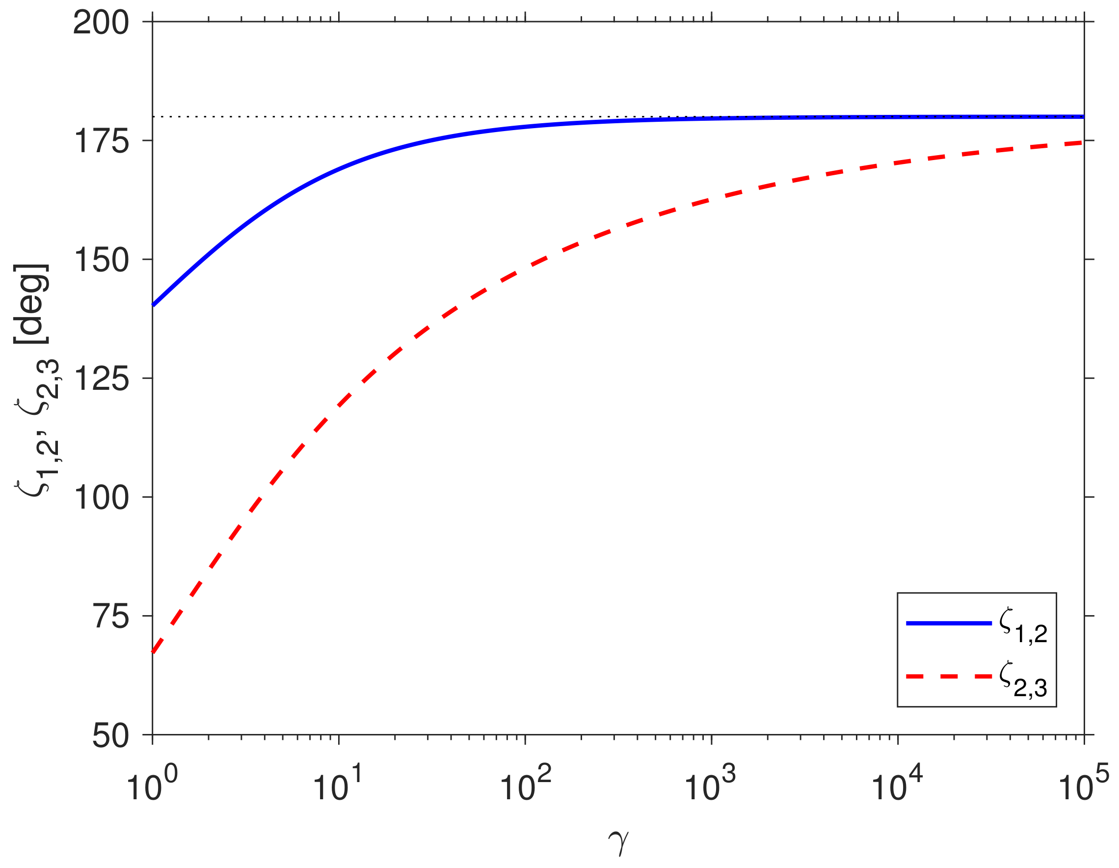
Figure 3 shows numerical values of the boost angles and as a function of . The angles increase from
and
at to as .
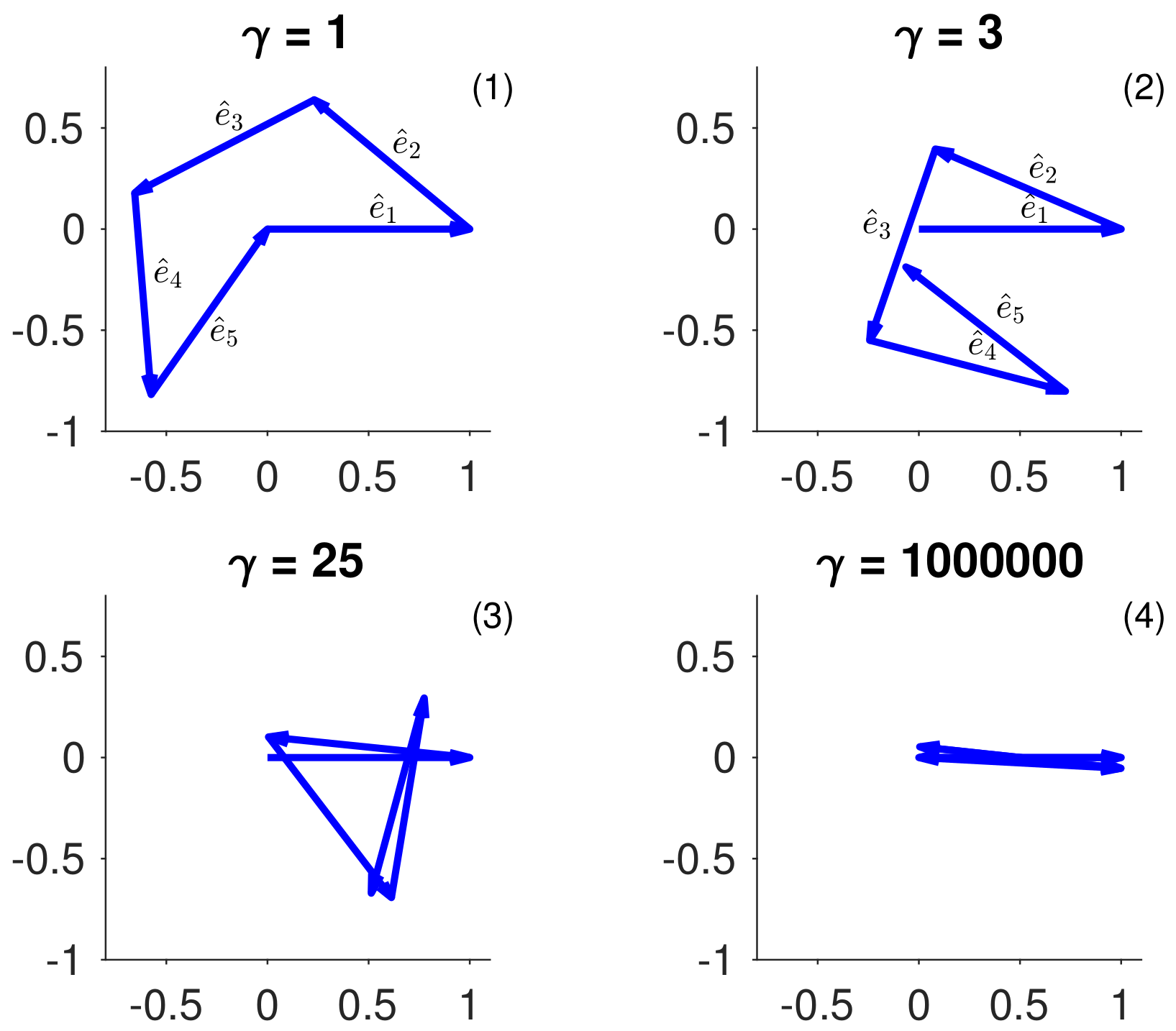
Figure 4 depicts the orientation of the five boost directions for several values of . Here, the first boost vector is taken to point along the x-axis. We note that the panels in Figure 4 do not represent a specific reference frame; rather, each vector is plotted with respect to frame (). The four panels show the changes in boost directions for increasing values of . Interestingly, the asymptotic limits and imply that in the relativistic limit the trajectory of R essentially reduces to one-dimensional motions along the x-axis. At the same time, the Thomas–Wigner rotation angle increases to as (see the discussion in Section 6 below).
Since the accelerated object is Born-rigid, the trajectories of all grid vertices G are uniquely determined once the trajectory of the reference point R is known [25,26,41]. Following the discussion in Section 3, the position and coordinate time of an arbitrary vertex G, in the frame comoving with R at the beginning of the corresponding acceleration phase, follows from Equation (10). The resulting trajectories are discussed in the next section.
5. Visualization
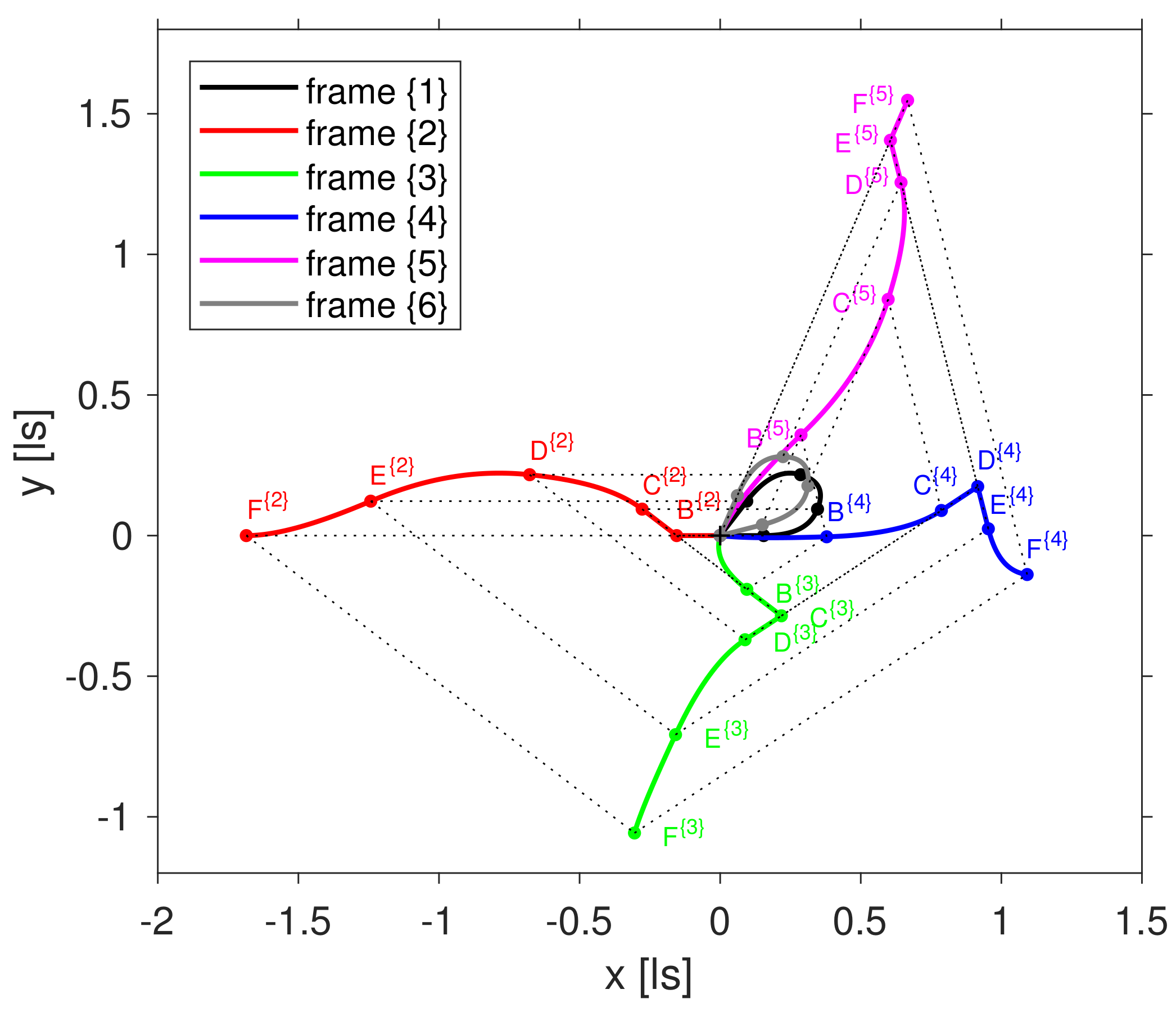
The trajectory of the reference point R in the laboratory frame for a boost speed , corresponding to , is displayed in Figure 1 (black solid line). The same trajectory as it appears to an observer in frame is marked in grey. The two frames are stationary with respect to each other, but rotated by a Thomas–Wigner angle of about . In addition, dots mark the locations of the four switchover events B, C, D and E in the two frames. As required by assumption 〈2〉, the starting and final positions, corresponding to the events A and F, coincide.
Figure 2 shows the same trajectories as Figure 1. In addition, R’s trajectories as recorded by observers in the frames are plotted as well (solid coloured lines). Corresponding switchover events are connected by dashed lines. At , , and (and, of course, at the start event and destination event ) the reference point R slows down and/or accelerates from zero velocity producing a kink in the trajectory. In all other cases, the tangent vectors of the trajectories, i.e., the velocities are continuous at the switchover points.
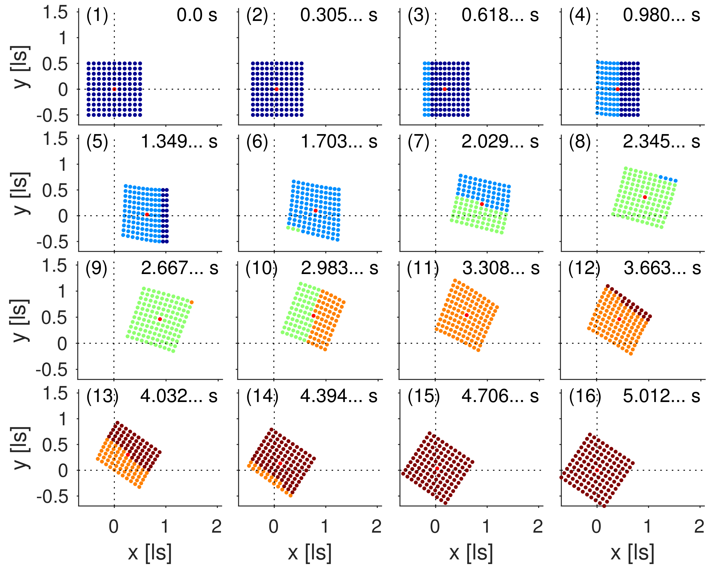
With Equations (30) and (34), all necessary ingredients to visualize the relativistic motion of a Born-rigid object are available. In Figure 5, the object is modelled as a square-shaped grid of points, arranged around the reference point R. The object uniformly accelerates in the -plane changing the boost direction four times by the angles (as measured in frame ), (frame ), (frame ) and finally (frame ). The vertices’ colour code indicates the corresponding boost section. The 16 panels depict the grid positions in the laboratory frame for specific values of coordinate time displayed in the top right.
To improve the visual impression, the magnitude of the Thomas–Wigner rotation in Figure 5 is enlarged by increasing the boost speed from , used in Figure 1 and Figure 2, to corresponding to . Despite its appearance, the grid is Born-rigid, and, in R’s MCIF, the grid maintains its original square shape. In the laboratory frame, however, appears compressed, when it starts to accelerate or decelerate and sheared, when one part of has not yet finished boost k, but the remaining part of already has transitioned to the next boost section . This feature is clearly evident from panels 4, 7, 10 or 13 in Figure 5 with the occurrence of two colours indicating two boost sections taking effect at the same epoch of coordinate laboratory time. We note, however, that the switchover events occur simultaneously for all grid points in R’s MCIF. The non-uniform colouring illustrate the non-simultaneity of the switchovers in the laboratory frame and thereby the relationship between Thomas–Wigner rotations and the non-existence of absolute simultaneity. A video animation is available online, details on how to access it are given in section “Supplementary Materials”.
6. Discussion
In this final section, the Thomas–Wigner rotation angle is calculated from the known boost angles and (Equation (35)). In addition, the maximum diameter of Born-rigid objects, Thomas–Wigner-rotated by a series of boosts, is discussed.
6.1. Derivation of Thomas–Wigner Angle
From the preceding sections follows a straightforward calculation of the Thomas–Wigner angle as a function of Lorentz factor . Assumption 〈2〉 implies that the sequence of the five Lorentz transformations is constructed such that frame is stationary with respect to frame and their spatial origins coincide. This means that the combined transformation reduces to an exclusively spatial rotation and the corresponding Lorentz matrix can be written as:
Since the rotation is confined to the -plane, the matrix elements with vanish. The remaining elements
yield the Thomas–Wigner rotation angle :
with denoting the four-quadrant inverse tangent. Equation (38) ensures that negative angles are unwrapped and mapped into the interval (see Figure 6).
With Equation (36), the rotation matrix elements and are found to be (see Appendix B)
and
with and given by Equations (30) and (34), respectively.
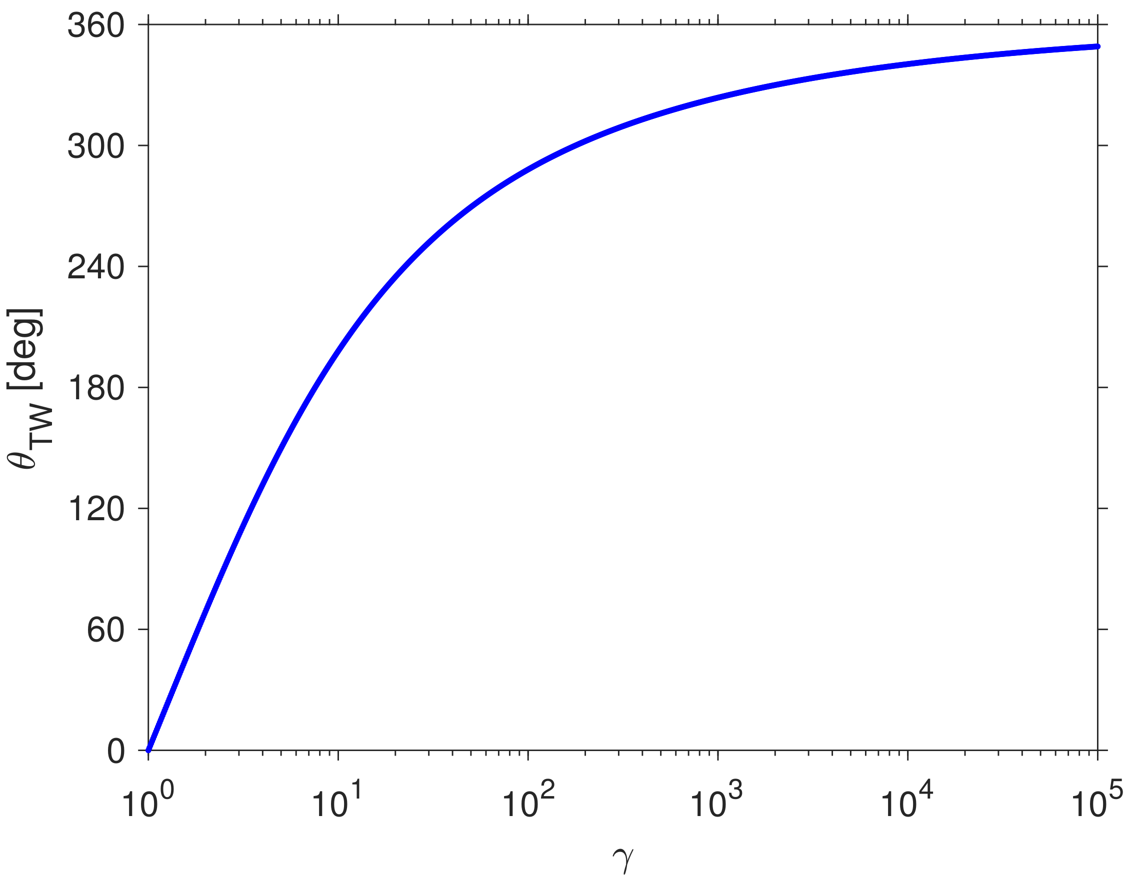
The resulting angle as a function of is plotted in Figure 6. The plot suggests that as . As already mentioned in Section 4 (see Figure 4), the boost angles and in the relativistic limit . Notwithstanding that R’s trajectory reduces to a one-dimensional motion as , the grid’s Thomas–Wigner rotation angle approaches a full revolution of in the laboratory frame.
6.2. Frame Boundaries
As illustrated by Figure 5, the Born-rigid object rotates in the -plane. Clearly, in order to preclude paradoxical faster-than-light translations of sufficiently distant vertices, ’s spatial extent in the x- and y-directions has to be bounded by a maximum distance from the reference point R on the order of [24]. As discussed in the following, this limit is put into effect by frame boundaries associated with ’s acceleration in each of the five boosts.
Figure 7 exemplifies the formation of a frame boundary for an accelerated object in (one time and one space) dimensions (see e.g., refs. [28,41,43,44]). Here, the Born-rigid object is assumed to be one-dimensional and to consist of seven equidistant grid points. Each point accelerates for a finite time period towards the positive x-direction (blue worldlines); the reference point R, marked in red, accelerates with . Contrary to the simulations discussed in Figure 5 above, for illustrative purposes, the acceleration phase is not followed immediately by another boost. Rather, the object continues to move with constant speed after the accelerating force has been switched off (green worldlines in Figure 7). The completion of the acceleration phase is synchronous in R’s MCIF (dashed-dotted line) and asynchronous in the laboratory frame. Figure 7 also illustrates that, for a uniform acceleration, the frame boundary (black dot) is stationary with respect to the laboratory frame.
In this simulation, each vertex is assumed to be equipped with an ideal clock ticking at a proper frequency of 10 Hz, the corresponding ticks are marked by dots; the boost phase lasts for 0.6 s on R’s clock. The clocks of the left-most (trailing) and right-most (leading) vertex measure (proper time) boost durations of 0.3 s and 0.9 s, respectively. Thus, with respect to the MCIFs (dashed lines), the vertex clocks run at different rates (see Equation (14)). The trailing clocks tick slower, the leading clocks faster than the reference clock at R. From Equations (13) and (14), it follows that the proper time variations are compensated by corresponding changes in proper acceleration experienced by the seven vertices. For the numerical values used in Figure 7, the accelerations of the trailing and leading vertex are and , respectively.
The spatial components of the inertial reference frames, comoving with R, are plotted in Figure 7 as well. During the acceleration-free period following the boost phase, the grid moves with constant speed and the equal-time slices of the corresponding comoving frames (dotted lines) are oriented parallel to each other. During the boost phase, however, the lines intersect and Equation (10) entails that the equal-time slices of the comoving frames all meet in one spacetime point; the frame boundary (black dot at ls and s in Figure 7).
If the accelerating grid extended to , the corresponding vertex would experience infinite proper acceleration (Equations (13) and (14)) and its clock would not tick. Clearly, a physical object accelerating towards positive x (Figure 7) cannot extend beyond this boundary at . If the grid in Figure 7 is regarded as realization of an accelerating coordinate system, this frame is bounded in the spatial dimension and ends at the coordinate value . However, as soon as the grid’s acceleration stops, the frame boundary disappears and coordinates are permissible. We note, that the frame boundary in Figure 7 is a zero-dimensional object, a point in -dimensional spacetime considered here. The boundary is frozen in time and exists only for the instant .
Generalizing this result, we find that the five boosts described in Section 4 and depicted in Figure 1 induce five frame boundaries in various orientations. It turns out that the accelerated object is completely surrounded by these boundaries within the -plane. They restrict ’s maximum size [24] and thereby assure that all of its vertices obey the special relativistic speed limit [4].
7. Conclusions
It is well known that pure Lorentz transformations do not form a group in the mathematical sense, since the composition of two transformations in general is not a pure Lorentz transformation again, but involves the Thomas–Wigner spatial rotation. The rotation is visualized by uniformly accelerating a Born-rigid object, consisting of a finite number of vertices, such that the object’s reference point returns to its starting location. It turns out that at least five boosts are necessary, provided, first, the (proper time) duration and the magnitude of the proper acceleration is the same within each boost and, second, the object’s motion is restricted to the -plane. Analytic expressions are derived for the angles between adjacent boost directions.
The visualization illustrates the relationship between Thomas–Wigner rotations and the relativity of simultaneity. The transition from one boost section to the next occurs synchronously in the MCIF of the object’s reference point. In the laboratory frame, however, the trailing vertices perform the transition to the next boost phase, which in general involves a direction change, earlier than the leading vertices. Thus, in this frame, the accelerated object not only contracts and expands along its direction of propagation, but also exhibits a shearing motion during the switchover phases. The simulations illustrate clearly that the aggregation of these shearing contributions finally adds up to the Thomas–Wigner rotation.
Accelerated motions induce frame boundaries, which no part of a physical, Born-rigid object may overstep. Thus, the object’s size is limited to a finite volume or area (if its motion is restricted to two spatial dimension) and Thomas–Wigner rotations by construction observe the special relativistic speed limit.
Supplementary Materials
An MPEG-4 video animation of the Thomas–Wigner rotation, the Matlab (Version 9, MathWorks Inc., Natick, MA, USA) source code used to create Figure 5 and the “SymPy” script file discussed in Appendix B are available at the URL www.gbeyerle.de/twr.
Acknowledgments
Valuable comments, suggestions and corrections by three anonymous reviewers are gratefully acknowledged. Several calculations of this study were performed with the computer algebra system “SymPy”, available at the URL www.sympy.org. “SymPy” is licensed under the General Public License; for more information, see www.gnu.org/licenses/gpl.html. All trademarks are the property of their respective owners.
Conflicts of Interest
The author declares no conflict of interest.
Abbreviations
| MCIF | momentarily comoving inertial frame |
Appendix A. Number of Boosts
We determine the smallest number of boosts that satisfies the four assumptions listed in Section 2. Denoting the number of boosts by N, it is self-evident that , since, for , the requirement of vanishing final velocity cannot be met if . In addition, for , the requirement of vanishing final velocity implies collinear boost directions. With two collinear boosts, however, the reference point R does not move along a non-trivial closed trajectory. In addition, we note that collinear boosts imply vanishing Thomas–Wigner rotation (see e.g., ref. [19]).
Appendix A.1. Three Boosts
Consider three boosts of the reference point R starting from location A and returning to location D via locations B and C. In the laboratory frame (frame ), the four-position at the destination D is given by
and
is the corresponding four-velocity. For the definition of the four-vector , see Equation (18). Assumption 〈2〉 implies that
and
Inserting Equation (1) into Equation (A2) yields
(see Appendix B) and, in turn, using Equation (A3) we obtain
Its only solution for real-valued is the trivial solution , i.e., . Thus, there are no non-trivial solutions for boosts, which are consistent with the assumptions 〈1〉–〈4〉.
Appendix A.2. Four Boosts
For a sequence of four boosts, time reversal symmetry implies that R’s velocity in the laboratory frame vanishes at event C after the second boost, i.e., . However, stationarity in the laboratory frame can only be achieved if the first two boosts and are collinear. In order to fulfil assumption 〈2〉 the third and fourth boosts have to be collinear with the first (and second) boost as well. As already noted, a sequence of collinear boosts, however, does not produce a non-zero Thomas–Wigner rotation.
Appendix B. Computer Algebra Calculations
Some equations in this paper were derived using the computer algebra system “SymPy” [45]. The corresponding “SymPy” source code files vtwr3bst.py (three boost case, see Appendix A.1) and vtwr5bst.py (five boost case, see Section 4) are available online, for details see section “Supplementary Materials”. These scripts process Equations (A1), (A2), (16) and (17) and derive the results given in Equations (A5), (A6), (23), (26), (27), (39) and (40). The following paragraphs provide a few explanatory comments.
First, we address the case of three boosts (superscript ) and the derivation of Equation (A5). The corresponding boost vectors in the -plane with are taken to be
with
in terms of the direction angle and the half-angle approximation (Equation (5)). Here, the z-coordinate is omitted since the trajectory is restricted to the -plane and from time reversal symmetry is being used. Inserting the corresponding Lorentz transformation matrices (Equation (1)) into Equation (A2) and selecting the time component yields
which reduces to Equation (A5) if the trivial solution is ignored.
For five boosts (superscript ) and the derivation of the expression (26), we define analogously to Equation (A7)
with
and
The corresponding Lorentz transformation matrices are too unwieldy to reproduce them here. “SymPy” script vtwr5bst.py calculates these matrices and their products in terms of and and inserts the result into Equation (17). The time component of Equation (17) yields the equation
We exclude the trivial solution and restrict ourselves to real values of and ; Equation (A13) then leads to Equation (22), a second order polynomial with respect to . The two solutions are given in Equation (23).
Next, we insert in Equation (16). Since its time component involves the travel time of R along its closed trajectory as an additional unknown and the z-coordinate vanishes by construction, we focus on the x- and y-components of Equation (16). The “SymPy” script vtwr5bst.py also shows that the result for the y-component of the equation can be expressed as
Here, , and are polynomials in .
For real and the numerator has to be zero. Moving the term involving the square root to the right-hand side and squaring both sides yields
Its evaluation (see script vtwr5bst.py) leads to the product of two polynomials (expressions (26) and (27)), each of which is of the fourth order with respect to .
Repeating the corresponding calculation for the x-component of the equation leads to the product of two polynomials, one of which is identical to expression (26). Thus, the roots of polynomial (26) constitute a solution of Equation (19). The Thomas–Wigner angle (Equation (38)) follows from the Lorentz matrix relating frame to frame (Equation (36)). The “SymPy” script vtwr5bst.py evaluates the matrix elements and in terms of and . Again, the resulting expressions are too unwieldy to reproduce them here.
References
- Tomonaga, S.-I. The Story of Spin; The University of Chicago Press: Chicago, IL, USA, 1997; ISBN 0-226-80794-0. [Google Scholar]
- Thomas, L.H. The motion of the spinning electron. Nature 1926, 117, 514. [Google Scholar] [CrossRef]
- Thomas, L.H. The kinematics of an electron with an axis. Philos. Mag. 1927, 3, 1–22. [Google Scholar] [CrossRef]
- Einstein, A. Zur Elektrodynamik bewegter Körper. Ann. Phys. 1905, 322, 891–921. [Google Scholar] [CrossRef]
- Wigner, E.P. On unitary representations of the inhomogeneous Lorentz group. Ann. Math. 1939, 40, 149–204. [Google Scholar] [CrossRef]
- Ben-Menahem, A. Wigners rotation revisited. Am. J. Phys. 1985, 53, 62–66. [Google Scholar] [CrossRef]
- Costella, J.P.; McKellar, B.H.J.; Rawlinson, A.A.; Stephenson, G.J., Jr. The Thomas rotation. Am. J. Phys. 2001, 69, 837–847. [Google Scholar] [CrossRef]
- Cushing, J.T. Vector Lorentz transformations. Am. J. Phys. 1967, 35, 858–862. [Google Scholar] [CrossRef]
- Ferraro, R.; Thibeault, M. Generic composition of boosts: An elementary derivation of the Wigner rotation. Eur. J. Phys. 1999, 20, 143–151. [Google Scholar] [CrossRef]
- Fisher, G.P. The Thomas precession. Am. J. Phys. 1972, 40, 1772–1781. [Google Scholar] [CrossRef]
- Gelman, H. Sequences of co-moving Lorentz frames. J. Math. Anal. Appl. 1990, 145, 524–538. [Google Scholar] [CrossRef]
- Gourgoulhon, E. Special Relativity in General Frames; Springer: Berlin, Germany, 2013. [Google Scholar]
- Kennedy, W.L. Thomas rotation: A Lorentz matrix approach. Eur. J. Phys. 2002, 23, 235–247. [Google Scholar] [CrossRef]
- Misner, C.W.; Thorne, K.S.; Wheeler, J.A. Gravitation; W. H. Freeman and Company: New York, NY, USA, 1973; ISBN 978-0716703440. [Google Scholar]
- Mocanu, C.I. On the relativistic velocity composition paradox and the Thomas rotation. Found. Phys. Lett. 1992, 5, 443–456. [Google Scholar] [CrossRef]
- Rȩbilas, K. Thomas precession and torque. Am. J. Phys. 2015, 83, 199–204. [Google Scholar] [CrossRef]
- Rhodes, J.A.; Semon, M.D. Relativistic velocity space, Wigner rotation, and Thomas precession. Am. J. Phys. 2004, 72, 943–960. [Google Scholar] [CrossRef]
- Rowe, E.G.P. The Thomas precession. Eur. J. Phys. 1984, 5, 40–45. [Google Scholar] [CrossRef]
- Steane, A.M. Relativity Made Relatively Easy; Oxford University Press: Oxford, UK, 2012; ISBN 019966286X. [Google Scholar]
- Ungar, A.A. The relativistic velocity composition paradox and the Thomas rotation. Found. Phys. 1989, 19, 1385–1396. [Google Scholar] [CrossRef]
- Ungar, A.A. Thomas precession: Its underlying gyrogroup axioms and their use in hyperbolic geometry and relativistic physics. Found. Phys. 1997, 27, 881–951. [Google Scholar] [CrossRef]
- Jonsson, R.M. Gyroscope precession in special and general relativity from basic principles. Am. J. Phys. 2007, 75, 463–471. [Google Scholar] [CrossRef]
- Koks, D. Explorations in Mathematical Physics: The Concepts Behind an Elegant Language; Springer: New York, NY, USA, 2006; ISBN 978-0-387-30943-9. [Google Scholar]
- Born, M. Die Theorie des starren Elektrons in der Kinematik des Relativitätsprinzips. Annalen der Physik 1909, 335, 1–56. [Google Scholar] [CrossRef]
- Herglotz, G. Über den vom Standpunkt des Relativitätsprinzips aus als “starr” zu bezeichnenden Körper. Ann. Phys. 1909, 336, 393–415. [Google Scholar] [CrossRef]
- Noether, F. Zur Kinematik des starren Körpers in der Relativtheorie. Ann. Phys. 1910, 336, 919–944. [Google Scholar] [CrossRef]
- Koks, D. Simultaneity on the rotating disk. Found. Phys. 2017, 47, 505–531. [Google Scholar] [CrossRef]
- Hamilton, J.D. The uniformly accelerated reference frame. Am. J. Phys. 1978, 46, 83–89. [Google Scholar] [CrossRef]
- Hobson, M.P.; Efstathiou, G.P.; Lasenby, A.N. General Relativity: An Introduction for Physicists; Cambridge University Press: Cambridge, UK, 2006; ISBN 0-521-82951-8. [Google Scholar]
- Rindler, W. Relativity: Special, General, and Cosmological; Oxford University Press Inc.: New York, NY, USA, 2001. [Google Scholar]
- Styer, D.F. How do two moving clocks fall out of sync? A tale of trucks, threads, and twins. Am. J. Phys. 2007, 75, 805–814. [Google Scholar] [CrossRef]
- Dewan, E.; Beran, M. Note on stress effects due to relativistic contraction. Am. J. Phys. 1959, 27, 517–518. [Google Scholar] [CrossRef]
- Dewan, E.M. Stress effects due to Lorentz contraction. Am. J. Phys. 1963, 31, 383–386. [Google Scholar] [CrossRef]
- Bell, J.S. Speakable and Unspeakable in Quantum Mechanics, 2nd ed.; Cambridge University Press: Cambridge, UK, 2004; ISBN 978-0-521-52338-7. [Google Scholar]
- Franklin, J. Lorentz contraction, Bell’s spaceships and rigid body motion in special relativity. Eur. J. Phys. 2010, 31, 291–298. [Google Scholar] [CrossRef]
- Evett, A.A. A relativistic rocket discussion problem. Am. J. Phys. 1972, 40, 1170–1171. [Google Scholar] [CrossRef]
- Evett, A.A.; Wangsness, R.K. Note on the separation of relativistically moving rockets. Am. J. Phys. 1960, 28, 566. [Google Scholar] [CrossRef]
- Fernflores, F. Bell’s spaceships problem and the foundations of special relativity. Int. Stud. Philos. Sci. 2011, 25, 351–370. [Google Scholar] [CrossRef]
- Redz̆ić, D.V. Note on Dewan–Beran–Bell’s spaceship problem. Eur. J. Phys. 2008, 29, N11–N19. [Google Scholar] [CrossRef]
- Tartaglia, A.; Ruggiero, M.L. Lorentz contraction and accelerated systems. Eur. J. Phys. 2003, 24, 215–220. [Google Scholar] [CrossRef]
- Eriksen, E.; Mehlen, M.; Leinaas, J.M. Relativistic rigid motion in one dimension. Phys. Scr. 1982, 25, 905–910. [Google Scholar] [CrossRef]
- Wikipedia. Quartic Function. 2017. Available online: http://en.wikipedia.org/wiki/Quarticfunction (accessed on 10 November 2017).
- Desloge, E.A.; Philpott, R.J. Uniformly accelerated reference frames in special relativity. Am. J. Phys. 1987, 55, 252–261. [Google Scholar] [CrossRef]
- Semay, C. Observer with a constant proper acceleration. Eur. J. Phys. 2006, 27, 1157–1167. [Google Scholar] [CrossRef]
- Joyner, D.; Čertík, O.; Meurer, A.; Granger, B.E. Open source computer algebra systems: SymPy. ACM Commun. Comput. Algebra 2012, 45, 225–234. [Google Scholar] [CrossRef]
Figure 1.
Trajectories of reference point R for as seen from (laboratory) frame and frame . The two frames are stationary with respect to each other, but rotated by a Thomas–Wigner angle of .
Figure 1.
Trajectories of reference point R for as seen from (laboratory) frame and frame . The two frames are stationary with respect to each other, but rotated by a Thomas–Wigner angle of .
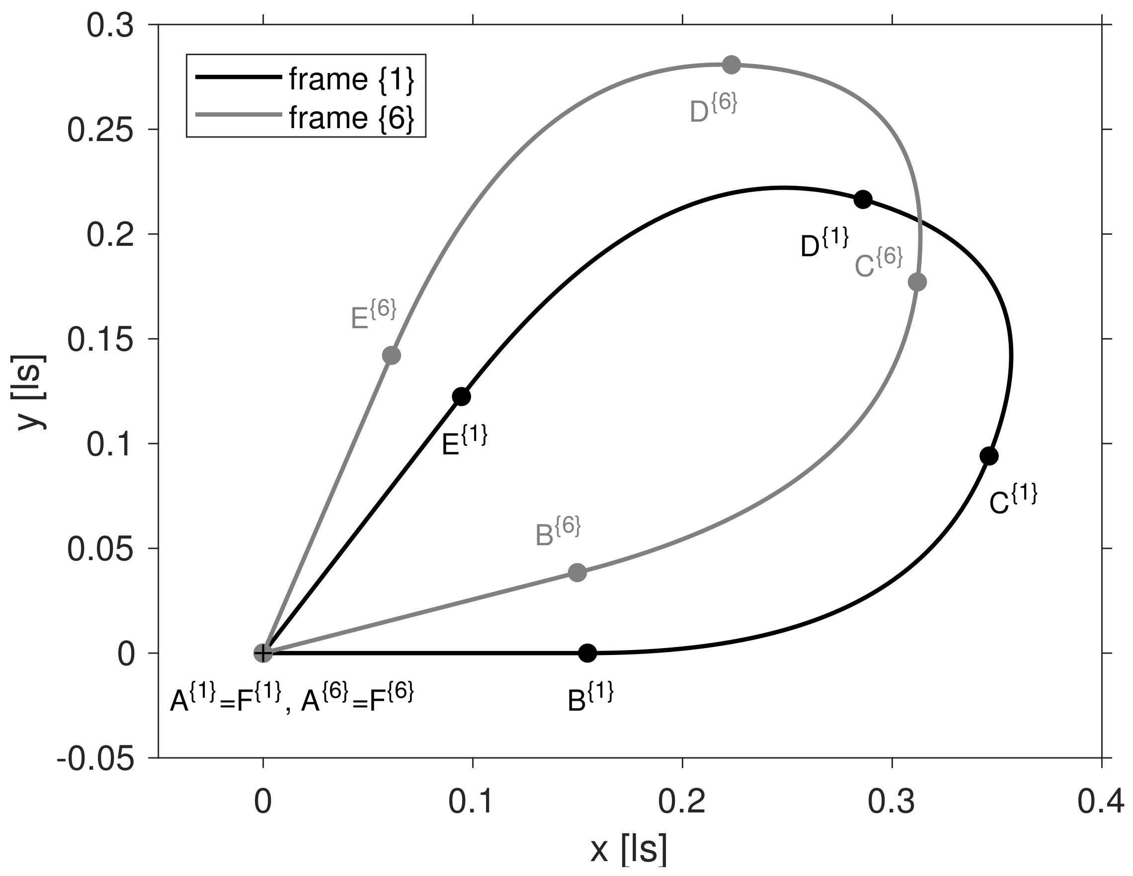
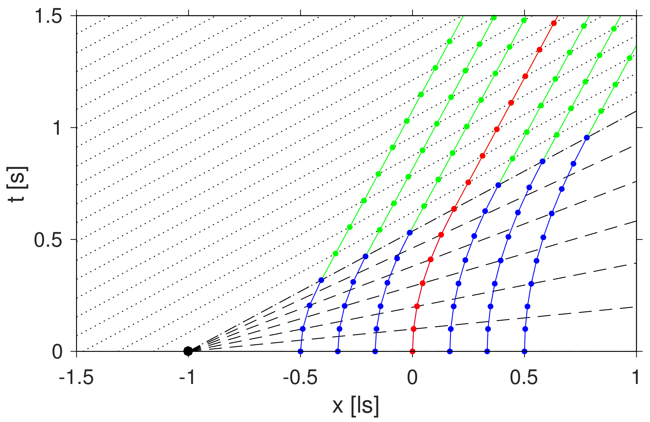
Figure 2.
Trajectories of the reference point R as seen from the six frames . The switchover points are marked by with . Corresponding switchover points are connected by dotted lines. The Lorentz factor is .
Figure 2.
Trajectories of the reference point R as seen from the six frames . The switchover points are marked by with . Corresponding switchover points are connected by dotted lines. The Lorentz factor is .

Figure 3.
The angle between the boost direction vectors and in frame (solid line), and the angle between and in frame (dashed line) as a function of . The dotted line marks , the limit of and for .
Figure 3.
The angle between the boost direction vectors and in frame (solid line), and the angle between and in frame (dashed line) as a function of . The dotted line marks , the limit of and for .

Figure 4.
Boost directions for four different values of . The boost direction in frame , is assumed to point along the x-axis. In the relativistic limit (panel 4) the angles between and approach . The motion of the reference point R tends to be more and more restricted along the x-axis and the object’s trajectory transitions from a two- to a one-dimensional motion.

Figure 5.
A series of grid positions as seen in the laboratory frame. The boost speed is taken to be , resulting in a Thomas–Wigner rotation angle of about . Coordinate time is displayed in the top right corner of each panel. The five boost phases are distinguished by colour. Evidently, switchovers between boosts do not occur simultaneously in the laboratory frame. The reference point (marked in red) moves along its trajectory counterclockwise, whereas the grid Thomas–Wigner rotates clockwise. For details, see text.

Figure 6.
Thomas–Wigner rotation angle as a function of . For clarity, the angle is unwrapped and mapped to the range .
Figure 6.
Thomas–Wigner rotation angle as a function of . For clarity, the angle is unwrapped and mapped to the range .

Figure 7.
Spacetime diagram of a one-dimensional grid consisting of seven points. The grid accelerates towards the positive x-direction. The trajectories are marked in blue/green, the mid point is taken as the reference R and its worldline is colored in red. Dots indicate the lapse of 0.1 s in proper time. After 0.6 s have passed on R’s clock, the acceleration stops and the points move with constant speed (green lines). Dashed and dotted lines connect simultaneous spacetime events in R’s comoving frame.

© 2017 by the author. Licensee MDPI, Basel, Switzerland. This article is an open access article distributed under the terms and conditions of the Creative Commons Attribution (CC BY) license (http://creativecommons.org/licenses/by/4.0/).
Share and Cite
MDPI and ACS Style
Beyerle, G. Visualization of Thomas–Wigner Rotations. Symmetry 2017, 9, 292. https://doi.org/10.3390/sym9120292
AMA Style
Beyerle G. Visualization of Thomas–Wigner Rotations. Symmetry. 2017; 9(12):292. https://doi.org/10.3390/sym9120292
Chicago/Turabian StyleBeyerle, Georg. 2017. "Visualization of Thomas–Wigner Rotations" Symmetry 9, no. 12: 292. https://doi.org/10.3390/sym9120292
Note that from the first issue of 2016, this journal uses article numbers instead of page numbers. See further details here.