Open Gromov-Witten Invariants from the Augmentation Polynomial

Abstract

A conjecture of Aganagic and Vafa relates the open Gromov-Witten theory of $X={\mathcal{O}}_{{\mathbb{P}}^1}(-1,-1)$ to the augmentation polynomial of Legendrian contact homology. We describe how to use this conjecture to compute genus zero, one boundary component open Gromov-Witten invariants for Lagrangian submanifolds $L_K\subset X$ obtained from the conormal bundles of knots $K\subset S^3$. This computation is then performed for two non-toric examples (the figure-eight and three-twist knots). For $(r,s)$ torus knots, the open Gromov-Witten invariants can also be computed using Atiyah-Bott localization. Using this result for the unknot and the $(3,2)$ torus knot, we show that the augmentation polynomial can be derived from these open Gromov-Witten invariants.

1. Introduction

Gromov-Witten theory has famously benefited from its connections with string dualities, first with mirror symmetry [1,2], and more recently, large N duality [3,4]. Beginning with [5], for toric manifolds, Gromov-Witten invariants associated with maps of closed surfaces have also been systematically computed using localization [6,7,8]. Although the analogous constructions in open Gromov-Witten theory are not rigorously defined in general, many of the same computational tools (such as mirror symmetry and Atiyah-Bott localization) can still be applied. In contrast to the closed theory, open Gromov-Witten theory also possesses many direct relationships with knot theory. Large N duality relates Chern-Simons theory on $S^3$ to Gromov-Witten theory on $X={\mathcal{O}}_{{\mathbb{P}}^1}(-1,-1)$ via the conifold transition. Wilson loops in Chern-Simons theory on $S^3$ are also related to the HOMFLY polynomials of knots $K\subset S^3$ [9]. This relationship equates the colored HOMFLY polynomials of knots K with generating functions for open Gromov-Witten invariants of X with Lagrangian boundary $L_K$ obtained from the conormal bundle $N_K^{*}\subset T^{*}{S}^3$, and has been checked for torus knots in [10].

Recently, it has also been suggested that open Gromov–Witten theory is related to another type of knot invariant arising in Legendrian contact homology [11,12]. For a knot $K\subset S^3$, Legendrian contact homology associates a dga $\mathcal{A}\left({\mathsf{\Lambda }}_K\right)$ with its unit conormal bundle ${\mathsf{\Lambda }}_K\subset U^{*}{S}^3$. The unit conormal bundle ${\mathsf{\Lambda }}_K\approx T^2$ is a Legendrian submanifold of the unit cotangent bundle $U^{*}{S}^3$ (a contact manifold), and the differential on $\mathcal{A}\left({\mathsf{\Lambda }}_K\right)$ is obtained, roughly speaking, from counts of maps of holomorphic disks to ${\mathsf{\Lambda }}_K\times \mathbb{R}$. An augmentation of $\mathcal{A}\left({\mathsf{\Lambda }}_K\right)$ is a dga map $ϵ:\mathcal{A}\left({\mathsf{\Lambda }}_K\right)\to \mathbb{C}$, where $\mathbb{C}$ is interpreted as a dga with trivial differential. The moduli space of such augmentations is described by an equation $A_K\left(x,p,Q\right)=0$, where x, p, and Q are generators for $H_2(U^{*}{S}^3,{\mathsf{\Lambda }}_K)$. $A_K$ is called the augmentation polynomial of the knot K (more detailed accounts of Legendrian contact homology can be found in [12,13]).

Mirror symmetry is a relationship between two Calabi-Yau manifolds X and $\widehat{X}$ that identifies the symplectic structure on X with the complex structure on $\widehat{X}$, and vice versa (see [1,2]). The Strominger–Yau–Zaslow conjecture offers a geometric interpretation of mirror symmetry in terms of dual torus fibrations by special Lagrangian submanifolds [14]. When X is ${\mathcal{O}}_{{\mathbb{P}}^1}(-1,-1)$, the special Lagrangian fibers can be understood as originating from conormal bundles to unknots $K\subset S^3$ under large N duality [3,4]. In [11], Aganagic and Vafa generalize the Strominger-Yau-Zaslow conjecture to cases where the special Lagrangian fibers are obtained from arbitrary knots $K\subset S^3$ by identifying this moduli space with the augmentation polynomial $A_K$ of the knot. Mirror symmetry interprets this moduli space as the superpotential associated with the B-model topological string theory. The dual A-model theory’s superpotential contains the open Gromov-Witten invariants associated with $L_K$, so Aganagic and Vafa’s conjecture can be rephrased as follows:

Conjecture 1.

Let $K\subset S^3$ be a knot, and $L_K\subset X$ be a Lagrangian submanifold of $X={\mathcal{O}}_{{\mathbb{P}}^1}\left(-1,-1\right)$ with geometry $K\times {\mathbb{R}}^2$. Let $A_K$ denote the augmentation polynomial of K, and $W_K\left(x,Q\right)$ denote the genus-zero, one boundary component open Gromov–Witten potential

$$W_K\left(x,Q\right)=\sum _{d,w}{K}_{d,w}^{0,1}{Q}^d{x}^w.$$

Then,

$$\int -\log p\left(x,Q\right)\frac{dx}{x}=W_K\left(x,Q\right),$$

(1)

where $p\left(x,Q\right)$ is the function implicitly defined by the equation $A_K\left(x,p,Q\right)=0$. More generally, the moduli of Lagrangian branes with geometry $K\times {\mathbb{R}}^2$ is given by the equation

$$A_K\left(x,p,Q\right)=0,$$

and K determines a mirror manifold ${\widehat{X}}_K$ defined by the hypersurface

$${\widehat{X}}_K=\left\{uv=A_K\left(x,p,Q\right)\right\}\subset {\mathbb{C}}^4.$$

The goal of this paper is to use this conjecture to compute Gromov-Witten invariants and augmentation polynomials. Because the augmentation polynomial can be computed for non-toric knots, this method can be applied in scenarios where Atiyah-Bott localization cannot be used. On the other hand, for $(r,s)$ torus knots, open Gromov-Witten invariants are known from localization, and this data provides another means of obtaining the augmentation polynomial of K.

1.1. Statement of Main Results

The main result of this paper is a technique for computing open Gromov-Witten invariants using Conjecture 1. This technique is applied for two non-toric knots (the $4_1$ and $5_2$ knots) for which a direct approach using Atiyah-Bott localization is intractable.

Proposition 1.

Let $K_{d,w}$ denote the open Gromov-Witten invariants of degree d and winding w for the $4_1$ and $5_2$ knots in framing 0 computed using Conjecture 1. Then, for $w\le 8$ and all d, $K_{d,w}$ satisfy the integrality constraint

$$K_{d,w}=\sum _{n\left|d{\displaystyle and}n\right|w}\frac{1}{n^2}{N}_{d/n,w/n}.$$

(2)

While, for non-toric knots, $K_{d,w}$ cannot be found through localization (removing the possibility of comparison against direct computation), the integrality constraint (2) is a strong restriction satisfied by Gromov-Witten invariants. For a toric knot, the situation is better—a comparison with direct calculation can be made. This is done for two simple knots (the unknot and $(3,2)$ trefoil knot), and can (at least in theory) be done for any torus knot.

Proposition 2.

Let $K_{d,w}$ denote the open Gromov-Witten invariants of degree d and winding w for the unknot and $(3,2)$ torus knot. Then, for each knot, the augmentation polynomial $A_K$ can be recovered from the corresponding open Gromov-Witten invariants.

Note that, for an $(r,s)$ torus knot, the computational complexity of the algorithm used for this calculation scales quite poorly with increasing $r,s$, so there are practical limitations to obtaining augmentation polynomials for arbitrary torus knots in this way.

1.2. Organization of the Paper

This paper is organized in the following way. Section 2 reviews mirror symmetry for open Gromov-Witten invariants, and describes Aganagic and Vafa’s conjecture relating mirror symmetry and the augmentation polynomial. Section 3 applies this conjecture to compute open Gromov-Witten invariants in two non-toric examples. Finally, Section 4 performs the reverse of this computation: the open Gromov-Witten invariants associated to torus knots are used to recover the corresponding augmentation polynomials. (Note that, for $(r,s)$ torus knots, open Gromov-Witten invariants in framing $rs$ have been computed directly via localization in [10].)

2. Open String Mirror Symmetry and the Augmentation Polynomial

Recently, new developments in knot theory and open topological string theory have uncovered connections between open Gromov-Witten theory and knot theory [4,10,11,12]. The subject of interest in this note is open Gromov-Witten theory for Lagrangian submanifolds of $X={\mathcal{O}}_{{\mathbb{P}}^1}(-1,-1)$. Let $\mathsf{\Sigma }$ be a genus-zero Riemann surface with one boundary component. Denote by $K_{d,w}$ the open Gromov-Witten invariant associated with a stable map $f:\mathsf{\Sigma }\to X$ with Lagrangian boundary conditions on a Lagrangian submanifold $L\subset X$, where $d=\left[f\left(\mathsf{\Sigma }\right)\right]\in H_2\left(X,L\right)$ and $w=\left[f\left(\partial \mathsf{\Sigma }\right)\right]\in H_1\left(L\right)$. This section describes a technique for computing $K_{d,w}$ using a mirror symmetry conjecture [11,12].

X can be obtained by symplectic reduction on ${\mathbb{C}}^4$. Let $(z_1,z_2,z_3,z_4)$ be coordinates for ${\mathbb{C}}^4$, and let $S^1$ act on ${\mathbb{C}}^4$ with weights $(1,1,-1,-1)$; then,

$$X\cong \left\{{\left|z_1\right|}^2+{\left|z_2\right|}^2-{\left|z_3\right|}^2-{\left|z_4\right|}^2=r\right\}/S^1,$$

(3)

where $r\in {\mathbb{R}}_{>0}$. The coordinates on the base ${\mathbb{P}}^1$ are $z_1$ and $z_2$, and the $z_3$, $z_4$ coordinates parametrize the fiber. According to the Strominger-Yau-Zaslow conjecture for noncompact X [14,15], X is a special Lagrangian fibration over a base $B\cong {\mathbb{R}}^3$, with generic fibers $L\cong T^2\times \mathbb{R}$. In these coordinates, the base B and the special Lagrangian fibers L are easy to describe. The base B is the image of X under the moment map $z_i\mapsto {\left|z_i\right|}^2$, and the fibers L are given by the equations

$$\begin{array}{cc}\hfill {\left|z_2\right|}^2-{\left|z_4\right|}^2& =c_1,\hfill \\ \hfill {\left|z_3\right|}^2-{\left|z_4\right|}^2& =c_2,\hfill \\ \hfill \mathrm{Arg}\left(z_1{z}_2{z}_3{z}_4\right)& =0,\hfill \end{array}$$

(4)

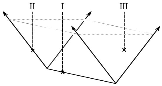
where $c_1,c_2\in \mathbb{R}$. For generic values of $c_1$, $c_2$, L has topology $T^2\times \mathbb{R}$; however, along a critical locus (such as when either $c_1\to 0$ or $c_2\to 0$), the topology of the fibers degenerates to two copies of $S^1\times {\mathbb{R}}^2$. This critical locus along which the fibers degenerate forms a trivalent graph in B, corresponding to the “edges” of the moment polytope. The moment polytope and special Lagrangian fibers are depicted in Figure 1.

Figure 1. The moment polytope and special Lagrangian fibers of X. The moment polytope of $X={\mathcal{O}}_{{\mathbb{P}}^1}(-1,-1)$ is its image $\pi \left(X\right)\subset {\mathbb{R}}^4$ under the moment map $\pi \left(z_i\right)={\left|z_i\right|}^2$. The images of the special Lagrangian fibers of X in the moment polytope are vertical lines, which can intersect X three ways: along the base ${\mathbb{P}}^1$ (type I), along an exterior leg of the polytope (type II), or on a face (type III). Lagrangian fibers of type III have topology $T^2\times \mathbb{R}$, corresponding to nondegenerate solutions in (4). Fibers of type I and II have topology $S^1\times {\mathbb{R}}^2$, corresponding to degenerate solutions (such as $c_2=0$ or $c_1=0$, respectively).

2.1. The Mirror of ${\mathcal{O}}_{{\mathbb{P}}^1}(-1,-1)$

The construction of [15,16] gives the mirror manifold $\widehat{X}$ to X in terms of a dual Landau-Ginsburg theory. For $X={\mathcal{O}}_{{\mathbb{P}}^1}(-1,-1)$, the mirror geometry is obtained from a $U\left(1\right)$ linear sigma model of four fields with charges $(1,1,-1,-1)$. The mirror geometry is described by

$$\widehat{X}=\left\{uv=y_2+y_3+y_4+\frac{y_3{y}_4}{y_2}{e}^{-t}\right\},$$

where $u,v\in \mathbb{C}$, $y_j\in {\mathbb{C}}^{*}$, $t=r+i\theta$ is the complexified Kähler parameter, and $y_1$ has been eliminated using the relation $y_1{y}_2=y_3{y}_4{e}^{-t}$. The Strominger-Yau-Zaslow (SYZ) conjecture [14] asserts that the mirror $\widehat{X}$ is the moduli of the special Lagrangian fibers of X. The choice of coordinate patch for the $y_j$’s determines which “phase” of Lagrangian fibers is being described. This coordinate choice is explained in further detail in [17]. In this note, the relevant coordinates are the $y_2=1$ patch. In addition, to achieve later agreement with conventions from knot contact homology, the following change of coordinates will be used:

$$\begin{array}{ccccc}\hfill Q:=e^t,& \hfill & \hfill x:=-y_3/Q,& \hfill & \hfill p:=-y_4/Q.\end{array}$$

Then, in this patch and coordinate system, the mirror manifold is

$$\widehat{X}=\left\{uv=1-Qx-Qp+Qxp\right\}.$$

(5)

Example 1 (Open Gromov-Witten invariants via mirror symmetry).

Consider Lagrangian fibers L of type II. These Lagrangians have topology $S^1\times {\mathbb{R}}^2$, and intersect the base ${\mathbb{P}}^1$ along the $S^1$. In the mirror, the moduli space of such Lagrangian fibers is the Riemann surface $S\subset \widehat{X}$ defined by setting $uv=0$:

$$S=\left\{1-Qx-Qp+Qxp=0\right\}.$$

Mirror symmetry equates the periods of certain differential forms on $\widehat{X}$ to generating functions for open Gromov–Witten invariants. In this case, the prediction of mirror symmetry is that (up to constant factors in x)

$$\int \lambda =\sum _{d,w}{K}_{d,w}{Q}^d{x}^w,$$

(6)

where $\lambda :=-\log p\frac{dx}{x}$ is a one-form along S defined by solving $1-Qx-Qp+Qxp=0$ for p, and $K_{d,w}$ is the genus-0, degree-d, winding w open Gromov-Witten invariant with boundary on L. In terms of x and Q,

$$\begin{array}{cc}\hfill -\log p\left(x;Q\right)& =\log \left(Q\right)+\log \left(\frac{1-x}{1-Qx}\right)\hfill \\ \hfill & =\log \left(Q\right)+\sum _{n=1}^{\infty }\frac{1}{n}\left(-1+Q^n\right)x^n,\hfill \end{array}$$

so Equation (6) asserts that

$$\sum _{d,w}{K}_{d,w}{Q}^d{x}^w=\sum _{n=1}^{\infty }\frac{1}{n^2}\left(-1+Q^n\right)x^n.$$

Hence,

$$K_{d,w}=\left\{\begin{array}{cc}-\frac{1}{w^2},\hfill & d=0,\hfill \\ \frac{1}{d^2},\hfill & d=w,\hfill \\ 0,\hfill & otherwise.\hfill \end{array}\right.$$

Note that, in this case, $K_{d,w}$ has also been computed directly using localization in [18], and these results agree in framing 0.

Open Gromov-Witten invariants are also conjectured to satisfy certain integrality requirements [15,19]. For genus-zero, one-boundary-component invariants, the requirement is that

$$K_{d,w}=\sum _{n\left|d{\displaystyle \mathrm{and}}n\right|w}\frac{1}{n^2}{N}_{d/n,w/n},$$

(7)

where $N_{d,w}\in \mathbb{Z}$. In terms of the generating function for $K_{d,w}$, this is

$$\sum _{d,w}{K}_{d,w}{Q}^d{x}^w=\sum _{n>0}\sum _{d,w}\frac{1}{n^2}{N}_{d,w}{Q}^d{x}^w.$$

In the previous example, $N_{0,1}=-1$, $N_{1,1}=1$, and $N_{d,w}=0$ for all other d, w.

2.2. Knots and the Conifold Transition

The Lagrangian submanifolds described by Equation (4) have a very specific geometry. A natural question is: What are the open Gromov-Witten invariants associated with Lagrangians with a different geometry? One way of obtaining such Lagrangians is through the conifold transition [4,10]. The manifold $X={\mathcal{O}}_{{\mathbb{P}}^1}(-1,-1)$ can also be obtained as the resolution of the conifold singularity in ${\mathbb{C}}^4$—it is given by the equations

$$\begin{array}{cc}\hfill xz-yw& =0,\hfill \\ \hfill x\lambda & =w\rho ,\hfill \\ \hfill y\lambda & =z\rho ,\hfill \end{array}$$

where $\left((x,y,z,w),\left[\lambda :\rho \right]\right)\in {\mathbb{C}}^4\times {\mathbb{P}}^1$ . The conifold singularity $xz-yw=0$ is the limit of the hypersurface

$$Y_{\mu }:=\left\{xz-yw=\mu \right\}\subset {\mathbb{C}}^4$$

as $\mu \to 0$. For $\mu \ne 0$, $Y_{\mu }$ is symplectomorphic to the cotangent bundle $T^{*}{S}^3$. The zero section $S_{\mu }\cong S^3\subset Y_{\mu }$ is the fixed locus of the antiholomorphic involution $(x,y,z,w)\mapsto (\overline{z},-\overline{w},\overline{x},-\overline{y})$, and is described by the equation ${\left|x\right|}^2+{\left|y\right|}^2=\mu$. Away from the zero sections, the conifold transition gives a map between $T^{*}{S}^3$ and X [10]. Consequently, a Lagrangian submanifold of $T^{*}{S}^3$ that does not intersect the zero section $S^3$ can be identified with a Lagrangian submanifold of X, which also does not intersect the zero section.

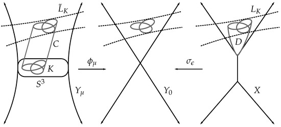
Knots $K\subset S^3$ are a source of Lagrangian submanifolds in $T^{*}{S}^3$: the conormal bundle $N_K^{*}\subset T^{*}{S}^3$ is Lagrangian with topology $S^1\times {\mathbb{R}}^2$. In order to obtain a Lagrangian submanifold of X from $N_K^{*}$, $N_K^{*}$ must first be moved off of the zero section. This can be done by choosing a lift of K, as described in [10]. The image of the shifted conormal bundle will be a Lagrangian submanifold $L_K\subset X$, as depicted in Figure 2.

Figure 2. The conifold transition and knots. The Lagrangian ${\tilde{L}}_K\subset Y_{\mu }\cong T^{*}{S}^3$ is constructed by shifting the conormal bundle of a knot $K\subset S^3$ off of the zero section. This lift introduces a holomorphic cylinder C connecting the knot on $S^3$ to its image in ${\tilde{L}}_K$. $Y_0$ is the conifold singularity $xz-yw=0$ in ${\mathbb{C}}^4$. The map ${\varphi }_{\mu }:Y_{\mu }\to Y_0$ is a symplectomorphism away from the zero section, so ${\varphi }_{\mu }({\tilde{L}}_K)$ is a Lagrangian submanifold of $Y_0$. $X\cong {\mathcal{O}}_{{\mathbb{P}}^1}(-1,-1)$ is the small resolution of the conifold singularity, and ${\sigma }_{ϵ}:X\to Y_0$ is the corresponding natural map. In fact, there are a family of such maps, where $ϵ$ parametrizes the symplectic area of the zero section ${\mathbb{P}}^1\subset X$. Hence, $L_K:={\sigma }_{ϵ}^{-1}\circ {\varphi }_{\mu }({\tilde{L}}_K)$ is a Lagrangian submanifold of X. The holomorphic disk D is the image of C under the conifold transition.

2.3. Open Gromov-Witten Invariants and the Augmentation Polynomial

For torus knots, the corresponding open Gromov-Witten invariants of $(X,L_K)$ have been computed directly using localization in [10], and using mirror symmetry in [20,21]. However, the mirror symmetry approach of [20] does not readily generalize to non-toric knots. In this subsection, a recent conjecture of Aganagic and Vafa [11] is applied to compute open Gromov-Witten invariants via an analogous mirror symmetry computation. This approach uses the augmentation polynomial from Legendrian contact homology. In contrast to localization and the method of [20], this method can be applied for any knot whose augmentation polynomial is known—including non-toric knots.

The Aganagic–Vafa conjecture can be motivated by observing that the mirror to $\widehat{X}$ given in Equation (5) can be written as

$$\widehat{X}=\left\{uv=A(x,p;Q)\right\},$$

where $A(x,p;Q)=1-Qx-Qp+Qxp$ is the augmentation polynomial of the unknot in Legendrian contact homology [13,22]. The moduli of Lagrangian submanifolds with topology $S^1\times {\mathbb{R}}^2$ was described by the zero locus

$$\left\{A(x,p;Q)=0\right\}\subset \widehat{X}.$$

Moreover, the image of a shifted conormal bundle to the unknot under the conifold transition described in Section 2.2 is exactly one of these Lagrangian fibers [4,23]. Hence, one might speculate that the moduli of Lagrangian submanifolds $L_K\subset X$ obtained from the conormal bundles of other knots $K\subset S^3$ are given by the Riemann surface

$$\left\{A_K(x,p;Q)=0\right\},$$

where $A_K(x,p;Q)$ is the augmentation polynomial of the knot K.

Aganagic and Vafa then conjecture that, for each choice of knot, there is a corresponding mirror ${\widehat{X}}_K$ describing the moduli space of Lagrangian fibers with geometry $L_K$ along the singular locus, and that ${\widehat{X}}_K$ is described by

$${\widehat{X}}_K:=\left\{uv=A_K(x,p;Q)\right\}.$$

In addition to the apparent coincidence between the unknot’s augmentation polynomial and the mirror $\widehat{X}$, there are also physical arguments for this conjecture coming from the connections between topological string theory, Chern-Simons theory, and the HOMFLY polynomial [11,12,21,24]. The augmentation polynomial $A_K$ can be identified with the classical limit of the Q-deformed quantum A-polynomial, which satisfies an elimination condition on the Chern-Simons partition function in the presence of a Wilson loop coming from K. This Chern-Simons partition function can in turn be obtained from the colored HOMFLY polynomials of K, and is identified with the open Gromov-Witten generating function under the conifold transition.

For the purposes of computing genus-zero open Gromov-Witten invariants, the application of this conjecture is straightforward: as in Section 2.1, the open Gromov-Witten generating function is equated with the integral of a differential form:

$$\sum _{d,w}{K}_{d,w}{Q}^d{x}^w=\int -\log p(x;Q)\frac{dx}{x}.$$

However, $p(x;Q)$ is now determined by the equation

$$A_K(x,p;Q)=0.$$

The main difficulty is that $A_K(x,p;Q)$ may be a high-order polynomial in p, so it is not always feasible to find analytic solutions for p. Even for torus knots, this can be an obstacle: for an $(r,s)$ torus knot,

$$\begin{array}{cccc}\hfill degp& =\left(\begin{array}{c}r+s\\ s\end{array}\right),\hfill & \hfill degx& =\frac{degp}{r+s}\hfill \end{array}$$

(8)

are the maximum degrees [21].

Fortunately, to compute $K_{d,w}$ for a given d and w, only a series solution for p is needed. Suppose that

$$p(x;Q)=\exp \left(-\sum _{n=0}^{\infty }{W}_n\left(Q\right)x^n\right),$$

(9)

where $W_n\left(Q\right)$ is a polynomial in Q for $n>0$, and $W_0\left(Q\right)$ determines the overall scaling of p. (Note that in all considered examples, $W_0\left(Q\right)=\log \left(Q\right)$, i.e., $p(x;Q)\approx 1/Q+\cdots$). Then, substitute this expression into

$$A_K\left(x,p(x;Q);Q\right)=0.$$

The resulting expression will be a series in x, which can be solved by recursively finding the coefficients $W_n\left(Q\right)$—in general, the coefficient of $x^n$ will be a polynomial function of ${\left\{W_k\left(Q\right)\right\}}_{k\le n}$. The coefficients $W_n\left(Q\right)$ are related to the $K_{d,w}$ by

$$W_n\left(Q\right)=\sum _{d}n{K}_{d,w}{Q}^d.$$

For completeness, the integer invariants $N_{d,w}$ can be similarly determined from the $K_{d,w}$: Equation (7) can be re-written as

$$N_{d,w}=K_{d,w}-\sum _{\begin{array}{c}n\left|d{\displaystyle \mathrm{and}}n\right|w\\ n>1\end{array}}\frac{1}{n^2}{N}_{d/n,w/n},$$

so by starting with $N_{0,1}=K_{0,1}$, successive $N_{d,w}$ can be solved for. The following section uses this method to compute $K_{d,w}$ and $N_{d,w}$ for two non-toric knots.

3. Non-Toric Examples

As compared with Atiyah–Bott localization, one advantage of computing open Gromov–Witten invariants from the augmentation polynomial is that this technique does not require that the Lagrangian L is fixed by a torus action. Such Lagrangians can be obtained from the conormal bundles of non-toric knots. This section performs the computation of Section 2.3 for two non-toric knots: the $4_1$ (figure-eight) knot and the $5_2$ (three-twist) knot. In contrast to torus knots, these knots cannot be expressed as the link of the singularity $x^r-y^s=0$ in $S^3$ for any $r,s\in \mathbb{Z}$. For non-toric knots, it is not currently known how to directly compute the open Gromov–Witten invariants $K_{d,w}$ using localization. However, the invariants computed in the following examples have been checked to satisfy the integrality condition (7) for all $w\le 8$ and arbitrary d, and the results may be compared against the colored HOMFLY polynomials in the symmetric representations.

3.1. The $4_1$ (Figure-Eight) Knot

The $4_1$ knot is the unique knot with crossing number 4, and is a twist knot obtained from two half-twists. According to [11,23], the augmentation polynomial of the $4_1$ knot in framing 0 is

$$\begin{array}{cc}\hfill A_K\left(x,p,Q\right)& =p^2-Q{p}^3+\left(Q^3{p}^5-2Q^3{p}^4+2Qp-Q\right)x\hfill \\ & +\left(-Q^5{p}^5+2Q^4{p}^4-2Q^{3}p+Q^2\right)x^2\hfill \\ & +\left(Q^5{p}^3-Q^5{p}^2\right)x^3.\hfill \end{array}$$

Rescaling x by $x\mapsto Qx$, one can obtain a series solution for $-\log p$ using the method of Section 2.3. The first few terms are

$$\begin{array}{cc}\hfill -\log p& =\log \left(Q\right)+\left(Q^3-2Q^2+2Q-1\right)x\hfill \\ & +\left(\frac{5Q^6}{2}-8Q^5+9Q^4-9Q^2+8Q-\frac{5}{2}\right)x^2+\cdots \hfill \end{array}$$

The coefficients of this series solution determine the open Gromov–Witten invariants $K_{d,w}$ and corresponding integer invariants $N_{d,w}$. For $w\le 4$, $0\le d\le 3$, these invariants are listed in Table 1 and Table 2. The integrality condition $N_{d,w}\in \mathbb{Z}$ has also been verified for all $w\le 8$ and arbitrary d. Note that, for $w\le 8$, $K_{d,w}=N_{d,w}=0$ for any $d>24$.

Table 1. $K_{d,w}$ for the $4_1$ knot.

${\mathit{K}}_{\mathit{d},\mathit{w}}$	${\mathit{K}}_{\mathit{d},1}$	${\mathit{K}}_{\mathit{d},2}$	${\mathit{K}}_{\mathit{d},3}$	${\mathit{K}}_{\mathit{d},4}$
$K_{0,w}$	$-1$	$-\frac{5}{4}$	$-\frac{28}{9}$	$-\frac{165}{16}$
$K_{1,3}$	2	4	14	60
$K_{2,w}$	$-2$	$-\frac{9}{2}$	$-25$	$-147$
$K_{3,w}$	1	0	$\frac{173}{9}$	186

Table 2. $N_{d,w}$ for the $4_1$ knot.

${\mathit{K}}_{\mathit{d},\mathit{w}}$	${\mathit{K}}_{\mathit{d},1}$	${\mathit{K}}_{\mathit{d},2}$	${\mathit{K}}_{\mathit{d},3}$	${\mathit{K}}_{\mathit{d},4}$
$K_{0,w}$	$-1$	$-\frac{5}{4}$	$-\frac{28}{9}$	$-\frac{165}{16}$
$K_{1,3}$	2	4	14	60
$K_{2,w}$	$-2$	$-\frac{9}{2}$	$-25$	$-147$
$K_{3,w}$	1	0	$\frac{173}{9}$	186

3.2. The $5_2$ (Three-Twist) Knot

The $5_2$ knot is a twist knot obtained from three half-twists, and is one of two knots with crossing number 5 (the other being the $(5,2)$ torus knot). The augmentation polynomial for the $5_2$ knot is

$$\begin{array}{cc}\hfill A_K(x,p,Q)& =Q^2{p}^8-Q{p}^7+x^4\left(-p+1\right)\hfill \\ & +\left(-Q^3{p}^6+2Q^2{p}^5-Q{p}^4-2Q{p}^3+3Q{p}^2-3p^2+4p-2\right)x^3\hfill \\ & +\left(Q^4{p}^8-3Q^3{p}^7-4Q^3{p}^6+5Q^2{p}^6+3Q^2{p}^5\right.\hfill \\ & \left.+6Q^2{p}^4-3Q{p}^5-4Q{p}^4+3Q{p}^3-4Q{p}^2-3p^3+5p^2-3p+1\right)x^2\hfill \\ & +\left(-2Q^3{p}^8+4Q^2{p}^7+3Q^2{p}^6-3Q{p}^6-2Q{p}^5-p^4+2p^3-p^2\right)x.\hfill \end{array}$$

Rescaling x by $x\mapsto x/Q$, the method of Section 2.3 gives a series solution for $-\log p$. The first few terms are

$$\begin{array}{cc}\hfill -\log p& =\log \left(Q\right)+\left(-Q^4+2Q^3-Q\right)x\hfill \\ & +\left(\frac{11Q^8}{2}-20Q^7+23Q^6-8Q^5+2Q^4-4Q^3+\frac{3Q^2}{2}\right)x^2+\cdots \hfill \end{array}$$

The corresponding $K_{d,w}$ and $N_{d,w}$ are obtained from the coefficients of this series solution. These invariants are listed in Table 3 and Table 4. As for the $4_1$ knot, the integrality condition $N_{d,w}\in \mathbb{Z}$ has also been checked for all $w\le 8$, and it was again found that $K_{d,w}=N_{d,w}=0$ for any $w\le 8$ and $d>24$.

Table 3. $K_{d,w}$ for the $5_2$ knot.

${\mathit{K}}_{\mathit{d},\mathit{w}}$	${\mathit{K}}_{\mathit{d},1}$	${\mathit{K}}_{\mathit{d},2}$	${\mathit{K}}_{\mathit{d},3}$	${\mathit{K}}_{\mathit{d},4}$
$K_{0,w}$	$-1$	$\frac{3}{4}$	$-\frac{10}{9}$	$\frac{35}{16}$
$K_{1,3}$	0	$-2$	4	$-12$
$K_{2,w}$	2	1	0	$\frac{27}{2}$
$K_{3,w}$	$-1$	$-4$	$-12$	8

Table 4. $N_{d,w}$ for the $5_2$ knot.

${\mathit{N}}_{\mathit{d},\mathit{w}}$	${\mathit{N}}_{\mathit{d},1}$	${\mathit{N}}_{\mathit{d},2}$	${\mathit{N}}_{\mathit{d},3}$	${\mathit{N}}_{\mathit{d},4}$
$N_{0,w}$	$-1$	1	$-1$	2
$N_{1,3}$	0	$-2$	4	$-12$
$N_{2,w}$	2	1	0	14
$N_{3,w}$	$-1$	$-4$	$-12$	8

4. Recovering the Augmentation Polynomial

The augmentation polynomial conjecturally contains all of the open Gromov-Witten invariants $K_{d,w}$ for a given Lagrangian brane $L_K$. As seen in the previous section, open Gromov-Witten invariants can be extracted from the augmentation polynomial. For torus knots, the genus zero open Gromov-Witten invariants can also be computed directly via localization. The formula is:

Lemma 1.

Suppose $\left(r,s\right)$ are coprime, $r>s>0$, and $ws\ge d>0$. Let K be the $\left(r,s\right)$ torus knot, and X, $L_K$, and $K_{d,w}$ as above. Then,

$$K_{d,w}={\left(-1\right)}^{d+1}\left(\frac{{\prod }_{k=0}^{d-1}\left(wr-k\right)\left(ws-k\right)}{wd!{\prod }_{k=1}^d\left(wr+ws-k\right)}\right)\left(\frac{{\prod }_{k=1}^{ws-1}\left(r+s-\frac{k}{w}\right)}{w{\prod }_{k=0}^{ws-1}\left(s-\frac{k}{w}\right)}\right),$$

(10)

where $\left(r,s\right)$ are coprime, $r>s>0$ and $ws\ge d\ge 0$. For $d>ws$, $K_{d,w}=0$.

The proof of this lemma is postponed to the Appendix A.

This section describes a method for obtaining the augmentation polynomial $A_K$ when K is a torus knot, and implements this method for two examples (the unknot, and the $(3,2)$ torus knot).

The idea is to use Equations (9) and (10) to obtain a system of linear equations on the coefficients of the augmentation polynomial. Write

$$A_K(x,p;Q)=\sum _{j,k}{c}_{jk}{x}^j{\left(p(x;Q)\right)}^k,$$

(11)

where $c_{jk}$ is a rational polynomial in Q. Recall that, for torus knots, the degrees of x and p are given by Equation (8). Let

$$p(x;Q)=\frac{1}{Q}\exp \left(-\sum _{d,w}w{K}_{d,w}{Q}^d{x}^w\right)$$

and $W_n:={\sum }_{d\ge 0}n{K}_{d,n}{Q}^d$. Then, the coefficient of $x^n$ in a series expansion of ${\left(p(x;Q)\right)}^k$ is $P_n\left(k\right)/Q^k$, where

$$P_n\left(k\right):=\sum _{\begin{array}{c}{i}_1+2i_2+\cdots +n{i}_n=n\\ i_j\ge 0\end{array}}\left[\prod _{j=1}^n\frac{{(-1)}^{i_j}}{i_j!}{\left(k{W}_j\right)}^{i_j}\right],$$

and $P_0\left(k\right)=1$. Substituting this expression into Equation (11) gives a power series in x:

$$\begin{array}{cc}\hfill A_K(x,p;Q)& =\sum _{j,k}{c}_{jk}\left(\frac{x^j}{Q^k}\right)\left(\sum _{n\ge 0}{P}_n\left(k\right)x^n\right)\hfill \\ & =\sum _{n\ge 0}\left(\sum _{j=0}^n\sum _{k\ge 0}\frac{P_{n-j}\left(k\right)}{Q^k}{c}_{jk}\right)x^n.\hfill \end{array}$$

In order for $p(x;Q)$ to be a solution of $A_K(x,p;Q)=0$, the coefficient of $x^n$ for all n in the above expression must vanish. This gives a collection of linear equations in the $c_{jk}$:

$$\sum _{j=0}^n\sum _{k\ge 0}\frac{P_{n-j}\left(k\right)}{Q^k}{c}_{jk}=0,$$

(12)

which can be solved to determine the $c_{jk}$ up to an overall rescaling of the augmentation polynomial. (Note that such rescalings do not affect the solutions $p(x;Q)$, and hence do not affect the Gromov–Witten invariants). The following two examples implement this procedure for the unknot in framing 0 and the (3, 2) torus knot in framing 6. For both knots, this method recovers the expected augmentation polynomial. However, for the (3, 2) knot, due to computational complexity, some simplifying assumptions about the values of the $c_{jk}$ are made.

4.1. The Unknot

For the unknot, $degx=1$, $degp=1$, so there are four coefficients to solve for: $c_{00}$, $c_{01}$, $c_{10}$, and $c_{11}$. Here, the $W_n$ have a simple expression:

$$W_n=\frac{1}{n}\left(Q^n-1\right).$$

The first four linear equations from Equation (12) are:

$$\begin{array}{cccc}\hfill c_{00}+\frac{1}{Q}{c}_{01}& =0,\hfill & \hfill & (n=0),\hfill \\ \hfill \frac{1}{Q}(1-Q)c_{01}+c_{10}+\frac{1}{Q}{c}_{11}& =0,\hfill & \hfill & (n=1),\hfill \\ \hfill \frac{1}{Q}(1-Q)c_{01}+\frac{1}{Q}(1-Q)c_{11}& =0,\hfill & \hfill & (n=2,3).\hfill \end{array}$$

(The $n=2$ and $n=3$ equations both simplify to the same expression). With $c_{00}$ as the free variable, these equations become

$$\begin{array}{ccccc}\hfill c_{01}=-Q{c}_{00,}& \hfill & \hfill c_{10}=-Q{c}_{00},& \hfill & \hfill c_{11}=Q{c}_{00}.\end{array}$$

Normalizing to $c_{00}=1$ yields the expected augmentation polynomial of the unknot in framing 0:

$$A_K(x,p;Q)=1-Qx-Qp+Qxp.$$

4.2. The $(3,2)$ Torus Knot

The augmentation polynomial of the (3, 2) torus knot is

$$\begin{array}{cc}\hfill A_K\left(x,p;Q\right)& =1-Qp+\left(Q^5{p}^3-Q^5{p}^4+2Q^5{p}^5-2Q^6{p}^5-Q^6{p}^6+Q^7{p}^7\right)x\hfill \\ & +\left(Q^{10}{p}^{10}-Q^{10}{p}^9\right)x^2.\hfill \end{array}$$

For the $(3,2)$ torus knot, $degp=10$ and $degx=2$. Thus, $c_{jk}=0$ for all $j>2$ and $k>10$. Note that, in general, one would need to consider at least $\left(\mathrm{deg}p+1\right)\left(\mathrm{deg}x+1\right)$ equations to determine $c_{jk}$. Due to the increasing complexity of the equations involved, in this example, the following simplifying assumptions (These assumptions are made to simplify the computation presented here and in principle are not needed.) will be made: $c_{0k}=0$ for $k>1$, $c_{10}=c_{11}=c_{12}=0$, $c_{18}=c_{19}=c_{1,10}=0$, and $c_{2k}=0$ for $k<9$. Thus, the remaining nine “unknown” coefficients are $c_{00}$, $c_{01}$, $c_{13}$, $c_{14}$, $c_{15}$, $c_{16}$, $c_{17}$, $c_{29}$, and $c_{2,10}$. The first three equations from Equation (12) are:

$$\begin{array}{cc}\hfill c_{00}+\frac{1}{Q}{c}_{01}& =0,\hfill \\ \hfill \left(2Q^{-1}-3+Q\right)c_{01}+Q^{-3}{c}_{13}+Q^{-4}{c}_{14}+Q^{-5}{c}_{15}+Q^{-6}{c}_{16}+Q^{-7}{c}_{17}& =0,\hfill \\ \hfill \left(23Q^{-1}-62+59Q-23Q^2+3Q^3\right)c_{01}+\left(3Q^{-1}-9Q^{-2}+6Q^{-3}\right)c_{13}& \\ \hfill +\left(4Q^{-2}-12Q^{-3}+8Q^{-4}\right)c_{14}+\left(5Q^{-3}-15Q^{-4}+10Q^{-5}\right)c_{15}& \\ \hfill +\left(6Q^{-4}-18Q^{-5}+12Q^{-6}\right)c_{16}+\left(7Q^{-5}-21Q^{-6}+14Q^{-7}\right)c_{17}& \\ \hfill +Q^{-9}{c}_{29}+Q^{-10}{c}_{2,10}& =0.\hfill \end{array}$$

(For brevity, the remaining equations are omitted.) Solving for the $c_{ij}$ (with $c_{00}$ as the free variable), one finds

$$\begin{array}{cccccccc}\hfill c_{01}& =-Q{c}_{00},\hfill & \hfill c_{13}& =Q^5{c}_{00},\hfill & \hfill c_{14}& =-Q^5{c}_{00},\hfill & \hfill c_{15}& =\left(2Q^5-2Q^6\right)c_{00},\hfill \\ \hfill c_{16}& =-Q^6{c}_{00},\hfill & \hfill c_{17}& =Q^7{c}_{00},\hfill & \hfill c_{29}& =-Q^{10}{c}_{00},\hfill & \hfill c_{2,10}& =Q^{10}{c}_{00}.\hfill \end{array}$$

By normalizing to $c_{00}=1$, the expected coefficients of the augmentation polynomial,

$$\begin{array}{cccccccc}\hfill c_{01}& =-Q,\hfill & \hfill c_{13}& =Q^5,\hfill & \hfill c_{14}& =-Q^5,\hfill & \hfill c_{15}& =2Q^5-2Q^6,\hfill \\ \hfill c_{16}& =-Q^6,\hfill & \hfill c_{17}& =Q^7,\hfill & \hfill c_{29}& =-Q^{10},\hfill & \hfill c_{2,10}& =Q^{10},\hfill \end{array}$$

are obtained.

5. Conclusions

Because of the difficulties involved in the computation of open Gromov-Witten invariants, a comparison of the technique described here against direct calculation is only currently possible in the torus knot case. A comparison for the non-toric case will require new techniques in enumerative geometry to verify. However, in all cases considered here, the computed open invariants are shown to satisfy a strong integrality condition expected of Gromov-Witten invariants. This can be seen as evidence for Aganagic and Vafa’s conjecture (Conjecture 1). Moreover, in the torus knot case, the corresponding open Gromov-Witten invariants have been computed explicitly in Lemma 1, so a direct comparison is possible—and here agreement is seen, both by comparing the Gromov-Witten invariants against series terms obtained from the augmentation polynomial, and by using the Gromov-Witten invariants to produce the augmentation polynomial. In the latter case, this provides a generic algorithm for computing the augmentation polynomial of any $(r,s)$ torus knot.

References

- Candelas, P.; de la Ossa, X.C.; Green, P.S.; Parkes, L. A pair of Calabi-Yau manifolds as an exactly soluble superconformal theory. Nuclear Phys. B 1991, 359, 21–74. [Google Scholar] [CrossRef] [Scilit]
- Witten, E. Mirror manifolds and topological field theory. In Essays on Mirror Manifolds; International Press: Hong Kong, China, 1992; pp. 120–158. [Google Scholar]
- Gopakumar, R.; Vafa, C. On the gauge theory/geometry correspondence. Adv. Theor. Math. Phys. 1999, 3, 1415–1443. [Google Scholar] [CrossRef] [Scilit]
- Ooguri, H.; Vafa, C. Knot invariants and topological strings. Nuclear Phys. B 2000, 577, 419–438. [Google Scholar] [CrossRef] [Scilit]
- Kontsevich, M. Enumeration of rational curves via torus actions. In The Moduli Space of Curves (Texel Island, 1994); Birkhäuser Boston: Boston, MA, USA, 1995; Volume 129, pp. 335–368. [Google Scholar]
- Graber, T.; Pandharipande, R. Localization of virtual classes. Invent. Math. 1999, 135, 487–518. [Google Scholar] [CrossRef] [Scilit]
- Chiang, T.M.; Klemm, A.; Yau, S.T.; Zaslow, E. Local mirror symmetry: Calculations and interpretations. Adv. Theor. Math. Phys. 1999, 3, 495–565. [Google Scholar] [CrossRef] [Scilit]
- Klemm, A.; Zaslow, E. Local mirror symmetry at higher genus. arXiv, 1999; arXiv:hep-th/9906046.
- Witten, E. Quantum field theory and the Jones polynomial. Commun. Math. Phys. 1989, 121, 351–399. [Google Scholar] [CrossRef] [Scilit]
- Diaconescu, D.E.; Shende, V.; Vafa, C. Large N duality, Lagrangian cycles, and algebraic knots. Commun. Math. Phys. 2013, 319, 813–863. [Google Scholar] [CrossRef] [Scilit]
- Aganagic, M.; Vafa, C. Large N duality, mirror symmetry, and a Q-deformed A-polynomial for knots. arXiv, 2012; arXiv:1204.4709 [hep-th].
- Aganagic, M.; Ekholm, T.; Ng, L.; Vafa, C. Topological strings, D-model, and knot contact homology. Adv. Theor. Math. Phys. 2014, 18, 827–956. [Google Scholar]
- Ng, L. A topological introduction to knot contact homology. arXiv, 2012; arXiv:1210.4803 [math.GT].
- Strominger, A.; Yau, S.T.; Zaslow, E. Mirror symmetry is T-duality. Nuclear Phys. B 1996, 479, 243–259. [Google Scholar] [CrossRef] [Scilit]
- Aganagic, M.; Vafa, C. Mirror symmetry, D-branes and counting holomorphic discs. arXiv, 2000; arXiv:hep-th/0012041.
- Hori, K.; Vafa, C. Mirror symmetry. arXiv, 2000; arXiv:hep-th/0002222.
- Aganagic, M.; Klemm, A.; Vafa, C. Disk instantons, mirror symmetry and the duality web. Z. Naturforsch. A 2002, 57, 1–28. [Google Scholar] [CrossRef] [Scilit]
- Katz, S.; Liu, C.C.M. Enumerative geometry of stable maps with Lagrangian boundary conditions and multiple covers of the disc. Adv. Theor. Math. Phys. 2001, 5, 1–49. [Google Scholar] [CrossRef] [Scilit]
- Labastida, J.; Mariño, M.; Vafa, C. Knots, links and branes at large N. J. High Energy Phys. 2001, 2000. [Google Scholar] [CrossRef] [Scilit]
- Brini, A.; Eynard, B.; Mariño, M. Torus knots and mirror symmetry. Ann. Henri Poincaré 2012, 13, 1873–1910. [Google Scholar] [CrossRef] [Scilit]
- Jockers, H.; Klemm, A.; Soroush, M. Torus knots and the topological vertex. Lett. Math. Phys. 2014, 104, 953–989. [Google Scholar] [CrossRef] [Scilit]
- Ekholm, T.; Etnyre, J.; Ng, L.; Sullivan, M. Knot contact homology. Geom. Topol. 2013, 17, 975–1112. [Google Scholar] [CrossRef] [Scilit]
- Gu, J.; Jockers, H.; Klemm, A.; Soroush, M. Knot invariants from topological recursion on augmentation varieties. Commun. Math. Phys. 2015, 336, 987–1051. [Google Scholar] [CrossRef] [Scilit]
- Neitzke, A.; Walcher, J. background independence and the open topological string wavefunction. arXiv, 2007; arXiv:0709.2390 [hep-th].
- Graber, T.; Zaslow, E. Open-string Gromov-Witten invariants: calculations and a mirror “theorem”. In Orbifolds in Mathematics and Physics (Madison, WI, 2001); American Mathematical Society: Providence, RI, USA, 2002; Volume 310, pp. 107–121. [Google Scholar]
- Givental, A. Equivariant Gromov-Witten invariants. Internat. Math. Res. Notices 1996, 1996, 613–663. [Google Scholar] [CrossRef]
- Brini, A.; Cavalieri, R. Open orbifold Gromov–Witten invariants of []: Localization and Mirror Symmetry. arXiv, 2010; arXiv:1007.0934 [math.AG].
- Brini, A. Open topological strings and integrable hierarchies: remodeling the A-model. Commun. Math. Phys. 2012, 312, 735–780. [Google Scholar] [CrossRef] [Scilit]
- Cox, D.A.; Katz, S. Mirror symmetry and algebraic geometry. In Mathematical Surveys and Monographs; American Mathematical Society: Providence, RI, USA, 1999; Volume 68. [Google Scholar]
- Coates, T.; Corti, A.; Iritani, H.; Tseng, H.H. Computing genus-zero twisted Gromov-Witten invariants. Duke Math. J. 2009, 147, 377–438. [Google Scholar] [CrossRef] [Scilit]
- Brini, A. (Imperial College London). Personal communication, 2016.
© 2017 by the author. Licensee MDPI, Basel, Switzerland. This article is an open access article distributed under the terms and conditions of the Creative Commons Attribution (CC BY) license (http://creativecommons.org/licenses/by/4.0/).