A Generalization of Trapezoidal Fuzzy Numbers Based on Modal Interval Theory

Abstract

We propose a generalization of trapezoidal fuzzy numbers based on modal interval theory, which we name “modal interval trapezoidal fuzzy numbers”. In this generalization, we accept that the alpha cuts associated with a trapezoidal fuzzy number can be modal intervals, also allowing that two interval modalities can be associated with a trapezoidal fuzzy number. In this context, it is difficult to maintain the traditional graphic representation of trapezoidal fuzzy numbers and we must use the interval plane in order to represent our modal interval trapezoidal fuzzy numbers graphically. Using this representation, we can correctly reflect the modality of the alpha cuts. We define some concepts from modal interval analysis and we study some of the related properties and structures, proving, among other things, that the inclusion relation provides a lattice structure on this set. We will also provide a semantic interpretation deduced from the modal interval extensions of real continuous functions and the semantic modal interval theorem. The application of modal intervals in the field of fuzzy numbers also provides a new perspective on and new applications of fuzzy numbers.

1. Introduction

The classical numerical system of real numbers is not efficient to express the vagueness, uncertainty and imprecision of real life. Fuzzy numbers and modal intervals are useful tools to get over those deficiencies.

The introduction of fuzzy sets by Zadeh [1] was a novelty as they provide a graduation of the membership relation. When considering fuzzy numbers, the expression “to be an element of a set” makes no sense, whereas many expressions in which this membership relation is relativized do indeed make sense.

Fuzzy numbers can be considered from two different points of view: with their membership function or with their $\alpha$-cuts. The two ways of considering fuzzy numbers are equivalent, and, depending on the details we want to study, one can be better than the other. Among all types of fuzzy numbers, triangular and trapezoidal ones, whose names are derived from the shape obtained when their membership function is represented in the Cartesian plane, are the most commonly used. However, when we observe a fuzzy number from the point of view of its $\alpha$-cuts, what we are indeed getting is an intervalar point of view of the fuzzy number.

Fuzzy sets theory has evolved since its appearance in 1965. Nowadays, we can find applications of fuzzy sets in the most part of scientific disciplines, such as decision-making [2,3,4], probability [5], control theory [6], medical sciences [7], characterization of complex systems [8], among others.

Modal intervals were introduced by Gardeñes [9] and they implied a new treatment of interval analysis, providing new resources to solve problems and systematize their resolution, as well as to interpret correctly an intervalar calculus.

Fuzzy numbers and intervals are not far removed from each other. This is because a fuzzy number can be identified by its $\alpha$-cuts, which are intervals, and intervals can also be considered fuzzy numbers.

The set of intervals, in their classical point of view, has some deficiencies in the operative sense and also in the interpretation of the calculus. These deficiences remain in the set of fuzzy numbers. Modal intervals, which are an extension of classical intervals, solve some of the operative deficiencies (although the distributive property is neither satisfied), and they give, without ambiguity, the right semantical interpretations of the calculus. Moreover, modal intervals are a lattice with regard to the incluson relationship, while classical intervals are not.

The advantages that present modal intervals in front of classical intervals have motivated us to deepen the relationship between fuzzy sets theory and interval analysis theory using modal intervals. We are certain that, with this tool, we open new lines of research.

If the connection between intervals and fuzzy numbers is so obvious, why not use modal intervals when working with fuzzy numbers, especially if we take into account the fact that modal intervals are an efficient extension of classical intervals? This is what we want to do in this paper: we will focus on the modal interval point of view of the $\alpha$-cuts of trapezoidal fuzzy numbers.

Modal intervals have been used combined with fuzzy sets [10,11]. The study that we present is based on the set of trapezoidal fuzzy numbers, expanding this set using modal intervals. The new fuzzy numbers obtained by this extension are named modal interval trapezoidal fuzzy numbers.

In this new set of modal interval trapezoidal fuzzy numbers (MITFNs), we study the inclusion relationship and we prove that this relationship provides a lattice structure. At the same time, in the set of MITFNs, we define the dual operator, inherited from the dual operator of modal intervals. The dual operator is an internal operator in the set of MITFNs, and it gives us the possibility to solve problems that, until now, had no solution in the set of traditional fuzzy numbers.

The rest of this paper is organized as follows. In Section 2, some basic concepts related to modal intervals and to fuzzy numbers are given. In Section 3, we provide the main definitions of this work and we also study the lattice structure of MITFNs with regard to the inclusion relation. In Section 4, we define the modal extension of a real function, we study some properties of this extension and we present the semantic interpretability theorem. Section 4 also includes an example to show some advantages when working on MITFNs instead of working with trapezoidal fuzzy numbers in their traditional sense. The conclusions and future research are described in Section 5.

2. Preliminaries

2.1. Modal Intervals

Given $a,b\in \mathbb{R}$ such that $a\le b$, the classical interval $\left[a,b\right]$ is defined as $\left[a,b\right]=\left\{x\in \mathbb{R}\mid a\le x\le b\right\}$. The set of classical intervals is represented by $I\left(\mathbb{R}\right)$ and it has been extensively studied. We can highlight the preliminary studies by Warmus [12] and Sunaga [13], and further consolidation of classical interval theory by Moore [14], Nickel [15] and Alefeld [16]. The operations between classical intervals have been studied by Kaucher [17].

Modal intervals were introduced by Gardeñes [9,18]. Some authors, such as Wang [19], refer to modal intervals as generalized intervals. A modal interval is defined as a pair consisting of a classical interval and a quantifier. The set of modal intervals is represented by $I^{\ast }\left(\mathbb{R}\right)$. Thus, $A\in I^{\ast }\left(\mathbb{R}\right)$ if $A=\left(\left[a,b\right],Q\right),$ where $\left[a,b\right]\in I\left(\mathbb{R}\right)$ and $Q\in \left\{\exists ,\forall \right\}.$ We can refer to $\left[a,b\right]$ as the subtractum of A, and it would be represented by $set\left(A\right)$; and we will refer to Q as the modality of A, which would be represented by $mod\left(A\right)$.

In the set of modal intervals, we distinguish proper intervals as those modal intervals whose modality is ∃; and improper intervals as those whose modality is ∀. Thus, A is proper if $A=\left(\left[a,b\right],\exists \right)$ and A is improper if $A=\left(\left[a,b\right],\forall \right)$. We identify proper intervals as the classical intervals. We will denote the proper interval $A=\left(\left[a,b\right],\exists \right)$ by $A=\left[a,b\right]$, and the improper interval $A=\left(\left[a,b\right],\forall \right)$ by $A=\left[b,a\right]$. Using this notation, the interval $\left[2,4\right]$ is the proper interval $\left(\left[2,4\right],\exists \right)$ and the interval $\left[3,1\right]$ is the improper interval $\left(\left[1,3\right],\forall \right)$. A pointwise interval can be considered as either proper or improper. Moore’s semiplane is useful to represent classical intervals, but it is not detailed enough to represent modal intervals, whose graphic representation must be in the interval plane (see Figure 1).

A modal interval A must be identified with the set of predicates accepted by A. Given a predicate P, this predicate is accepted by the modal interval $A=\left(\left[a,b\right],Q\right)$ if $Qx\in \left[a,b\right],P\left(x\right)$ is true. That is, if $A=\left(\left[a,b\right],\exists \right)$, P is a predicate accepted by A if $\exists x\in \left[a,b\right]$ such that $P\left(x\right)$ is true. In the same way, if $A=\left(\left[a,b\right],\forall \right),$ the predicate P is accepted by A if $\forall x\in \left[a,b\right],P\left(x\right)$ is true. We denote by $pred\left(A\right)$ the set of the predicates accepted by A.

The dual operator of a modal interval $A=\left(\left[a,b\right],Q\right)$, which we will represent by $du\left(A\right)$, is defined by $du\left(A\right)=\left(\left[a,b\right],du\left(Q\right)\right)$, where $du\left(Q\right)=\forall$ if $Q=\exists$ and $du\left(Q\right)=\exists$ if $Q=\forall$.

The inclusion relation between two modal intervals A and B is defined by:

$$A\subseteq B\iff pred\left(A\right)\subseteq pred\left(B\right)$$

and, using the canonical coordinates of A and B, the inclusion $A\subseteq B$ holds in the same way as in the set of classical intervals, that is, $\left[a,b\right]\subseteq \left[c,d\right]$ if $a\ge c$ and $b\le d.$

In the set of modal intervals, we define the meet $\left(\wedge \right)$ and join $\left(\vee \right)$ operators between two modal intervals. If $A=\left[a,b\right]$ and $B=\left[c,d\right]$, then $A\wedge B=\left[max\left\{a,c\right\},min\left\{b,d\right\}\right]$ and $A\vee B=\left[min\left\{a,c\right\},max\left\{b,d\right\}\right]$. The meet and join operators correspond to the intervalar infimum and supremum of two modal intervals with regard to the inclusion relation. Thus, the set of modal intervals is a lattice with regard to the inclusion relation, while the set of classical intervals is not.

Using the meet and join operators, we define the modal extension of a real continuous function $f:{\mathbb{R}}^n⟶\mathbb{R}$ which is represented by $f^{\ast }$ as:

$$f^{\ast }\left(X\right)=\underset{x_p\in set\left(X_P\right)}{\vee }\underset{x_i\in set\left(X_I\right)}{\wedge }\left[f\left(x_p,x_i\right),f\left(x_p,x_i\right)\right],$$

where $X_P$ are the proper components of X and $X_I$ are the improper ones.

The calculus of the modal extension of a real continuous function can be semantically interpreted using the semantic modal interval theorem [20].

2.2. Fuzzy Numbers

Fuzzy sets were introduced by Zadeh [1]. Although they are surely the most accepted tool to represent uncertainty, there are some other tools used to represent indiscernibility, vagueness, imprecision and also uncertainty: rough sets [21,22,23]; marks [24] and numerical clouds [25], among others.

If X is a universal set, a fuzzy set $A,$ in X can be defined by its membership function. The membership function of a fuzzy set A is a mapping ${\mu }_A:X\to \left[0,1\right]$ which assigns to each element $x\in X$, a real number ${\mu }_A\left(x\right)\in \left[0,1\right]$. The value ${\mu }_A\left(x\right)$ quantifies the level of membership of the fuzzy set A, of the element x.

A fuzzy number A is a fuzzy set of the real line. Its membership function, ${\mu }_A:\mathbb{R}\to \left[0,1\right]$ must be normal (that is, $\exists x\in \mathbb{R}$ such that ${\mu }_A\left(x\right)=1$), fuzzy convex ($\forall x,y\in \mathbb{R}\forall \lambda \in \left[0,1\right]$, ${\mu }_A\left(\lambda x+\left(1-\lambda \right)y\right)\ge {\mu }_A\left(x\right)\wedge {\mu }_A\left(y\right)$), upper semi-continuous and such that the closure of the set $\left\{x\in \mathbb{R}\mid {\mu }_A\left(x\right)>0\right\}$ is bounded [26].

The membership function of a fuzzy number A can be described as:

$${\mu }_A\left(x\right)=\left\{\begin{array}{cc}{f}_L\left(x\right),& \mathrm{if}{a}_1\le x<a_2,\\ 1,& \mathrm{if}{a}_2\le x\le a_3,\\ f_U\left(x\right),& \mathrm{if}{a}_3<x\le a_4,\\ 0,& \mathrm{otherwise},\end{array}\right.$$

where $a_1,a_2,a_3$ and $a_4$ are real numbers such that $a_1<a_2\le a_3<a_4$; $f_L$ is a real-valued strictly increasing and right-continuous function; and $f_U$ is a real-valued strictly decreasing and left-continuous function.

Given a fuzzy set A of X with membership function ${\mu }_A$, and given a real number $\alpha \in \left[0,1\right]$, the $\alpha$-cut of A is the crisp set denoted by $A^{\alpha }$ and is defined by:

$$A^{\alpha }=\left\{\begin{array}{cc}\left\{x\in X\mid {\mu }_A\left(x\right)\ge \alpha \right\},& \mathrm{if}\alpha \in \left(0,1\right],\hfill \\ \\ \overline{\left\{x\in X\mid {\mu }_A\left(x\right)>0\right\}},& \mathrm{if}\alpha =0,\hfill \end{array}\right.$$

where $\overline{\left\{x\in X\mid {\mu }_A\left(x\right)>0\right\}}$ is the closure of the set $\left\{x\in X\mid {\mu }_A\left(x\right)>0\right\}$.

The $\alpha$-cut $A^0$ is called the support of A and it is denoted by $supp\left(A\right).$ The $\alpha$-cut $A^1$ is called the core of A.

A fuzzy number A can be represented by its membership function or alternatively by the set of its $\alpha$-cuts: $A=\left\{A^{\alpha }\mid \alpha \in \left[0,1\right]\right\}.$

The expected interval of a fuzzy number is given by Dubois and Prade [27], Grzegorzewski [28], and Heilpern [29]. For a trapezoidal fuzzy number $A=\left(a_1,a_2,a_3,a_4\right)$, the expected interval is $EI\left(A\right)=\left[\frac{a_1+a_2}{2},\frac{a_3+a_4}{2}\right].$

3. Modal Interval Trapezoidal Fuzzy Numbers

Definition 1.

(Modal interval trapezoidal fuzzy number)

Given $\left[a_1,a_4\right],\left[a_2,a_3\right]\in I^{\ast }\left(\mathbb{R}\right)$ such that $set\left(\left[a_2,a_3\right]\right)\subseteq set\left(\left[a_1,a_4\right]\right)$.

If, for any $\alpha \in \left[0,1\right]$, we consider $A^{\alpha }=\left(1-\alpha \right)\left[a_1,a_4\right]+\alpha \left[a_2,a_3\right]$, then $A=\left\{A^{\alpha }\mid \alpha \in \left[0,1\right]\right\}$ is an MITFN which we represent by $A=\left(\left[a_1,a_4\right],\left[a_2,a_3\right]\right).$

The modal interval $\left[a_1,a_4\right]$ that corresponds to $A^0$ is the support of A, and the modal interval $\left[a_2,a_3\right]$ that corresponds to $A^1$ is the core of $A.$ Thus, $A=\left(A^0,A^1\right)$.

We denote the set of MITFNs by $T{I}^{\ast }\left(\mathbb{R}\right),$ extending the expression $I^{\ast }\left(\mathbb{R}\right),$ which denotes the set of modal intervals.

If $A=\left(\left[a_1,a_4\right],\left[a_2,a_3\right]\right)$ is an MITFN, we can define $set\left(A\right)$ as the trapezoidal fuzzy number (in its standard sense):

$$set\left(A\right)=\left(min\left\{a_1,a_4\right\},min\left\{a_2,a_3\right\},max\left\{a_2,a_3\right\},max\left\{a_1,a_4\right\}\right).$$

It is obvious that $supp\left(set\left(A\right)\right)=set\left(supp\left(A\right)\right)=set\left[a_1{a}_4\right]$ and $core\left(set\left(A\right)\right)=set\left(core\left(A\right)\right)=set\left[a_2,a_3\right].$

Definition 2.

(Modality of an MITFN)

Given $A=\left(\left[a_1,a_4\right],\left[a_2,a_3\right]\right)$ which is an MITFN, we define:

• A is a proper-improper MITFN (MITFN${}_P^I$) if $supp\left(A\right)$ is a proper interval and $core\left(A\right)$ is an improper interval. We denote it by $A=\left(set\left(A\right),\exists ,\forall \right)$;
• A is an improper-proper MITFN (MITFN${}_I^P$) if $supp\left(A\right)$ is an improper interval and $core\left(A\right)$ is a proper interval. We denote it by $A=\left(set\left(A\right),\forall ,\exists \right)$;
• A is a proper-proper MITFN (MITFN${}_P^P$) if both the support and core of A are proper intervals. We denote it by $A=\left(set\left(A\right),\exists ,\exists \right)$;
• A is an improper-improper MITFN (MITFN${}_I^I$) if both the support and core of A are improper intervals. We denote it by $A=\left(set\left(A\right),\forall ,\forall \right)$.

In general, an MITFN A will be:

$$A=\left(A^{\prime },Q_1,Q_2\right),$$

where $A^{\prime }$ is a trapezoidal fuzzy number in its traditional sense; $Q_1\in \left\{\exists ,\forall \right\}$ is the interval modality of the support of $A,$ that is, the modality of $\left[a_1,a_4\right]$; and $Q_2\in \left\{\exists ,\forall \right\}$ is the interval modality of the core of $A,$ that is, the modality of $\left[a_2,a_3\right]$.

If A is an MITFN${}_P^P$, we will refer to A as a proper trapezoidal fuzzy number; while if A is an MITFN${}_I^I$, then we will refer to A as an improper trapezoidal fuzzy number [10]. Notice that if A is an MITFN${}_P^P$, then A is a trapezoidal fuzzy number in its classical sense.

Proposition 1.

Given $A=\left(\left[a_1,a_4\right],\left[a_2,a_3\right]\right),$ which is an MITFN${}_P^I$ or an MITFN${}_I^P$, there exists a unique value ${\alpha }^0\in \left[0,1\right]$ such that the α-cut $A^{{\alpha }^0}$ is a pointwise interval $\left[p,p\right]$. Moreover, if $\beta \in \left[0,{\alpha }^0\right],$ then $mod\left(A^{\beta }\right)=mod\left(supp\left(A\right)\right)$ and if $\gamma \in \left[{\alpha }^0,1\right]$, then $mod\left(A^{\gamma }\right)=mod\left(core\left(A\right)\right).$

Proof. 

If A is an MITFN${}_P^I$, $a_1\le a_4$ and $a_2\ge a_3$. As $A^{\alpha }=\left(1-\alpha \right)\left[a_1,a_4\right]+\alpha \left[a_2,a_3\right]$.We must impose:

$$\left(1-\alpha \right)\left[a_1,a_4\right]+\alpha \left[a_2,a_3\right]=\left[p,p\right]\Rightarrow \left\{\begin{array}{c}\left(1-\alpha \right)a_1+\alpha a_2=p,\\ \left(1-\alpha \right)a_4+\alpha a_3=p,\end{array}\right.$$

that is:

$$\left\{\begin{array}{c}\alpha \left(a_2-a_1\right)-p=-a_1,\\ \alpha \left(a_3-a_4\right)-p=-a_4,\end{array}\right.$$

which has a unique solution as $\left|\begin{array}{cc}{a}_2-a_1& -1\\ a_3-a_4& -1\end{array}\right|\ne 0.$

Let ${\alpha }^0,p^0$ be the solution. If $\beta \in \left[0,{\alpha }^0\right]$, then $\beta ={\alpha }^0-\xi ,\xi \ge 0$. If A is an MITFN${}_P^I$, then we have to prove that $\left(1-\beta \right)\left[a_1,a_4\right]+\beta \left[a_2,a_3\right]$ is a proper interval. As $\left[a_1,a_4\right]$ is a proper interval, then $a_1-a_4\le 0$. As $\left[a_2,a_3\right]$ is an improper interval, then $a_2-a_3\ge 0:$

$$a_1-a_4\le a_2-a_3\Rightarrow a_1-a_2\le a_4-a_3$$

as $\xi \ge 0,$ $\xi \left(a_1-a_2\right)\le \xi \left(a_4-a_3\right)$ and

$$p^0+\xi a_1-\xi a_2\le p^0+\xi a_4-\xi a_3,$$

but $p^0$ is either $\left(1-{\alpha }^0\right)a_1+{\alpha }^0{a}_2$ or $\left(1-{\alpha }^0\right)a_4+{\alpha }^0{a}_3$, so it follows that:

$$\left(1-{\alpha }^0\right)a_1+{\alpha }^0{a}_2+\xi a_1-\xi a_2\le \left(1-{\alpha }^0\right)a_4+{\alpha }^0{a}_3+\xi a_4-\xi a_3$$

and then

$$\left(1-{\alpha }^0+\xi \right)a_1+\left({\alpha }^0-\xi \right)a_2\le \left(1-{\alpha }^0+\xi \right)a_4+\left({\alpha }^0-\xi \right)a_3,$$

so

$$\left(1-\beta \right)a_1+\beta a_2\le \left(1-\beta \right)a_4+\beta a_3,$$

which means that $A^{\beta }=\left[\left(1-\beta \right)a_1+\beta a_2,\left(1-\beta \right)a_4+\beta a_3\right]$ is a proper interval.

If $\gamma \in \left[{\alpha }^0,1\right]$, then $\gamma ={\alpha }^0+\xi ,\xi \ge 0$ and the demonstration would be equivalent.

Similar reasoning holds for the case in which A is an MITFN${}_I^P$. ☐

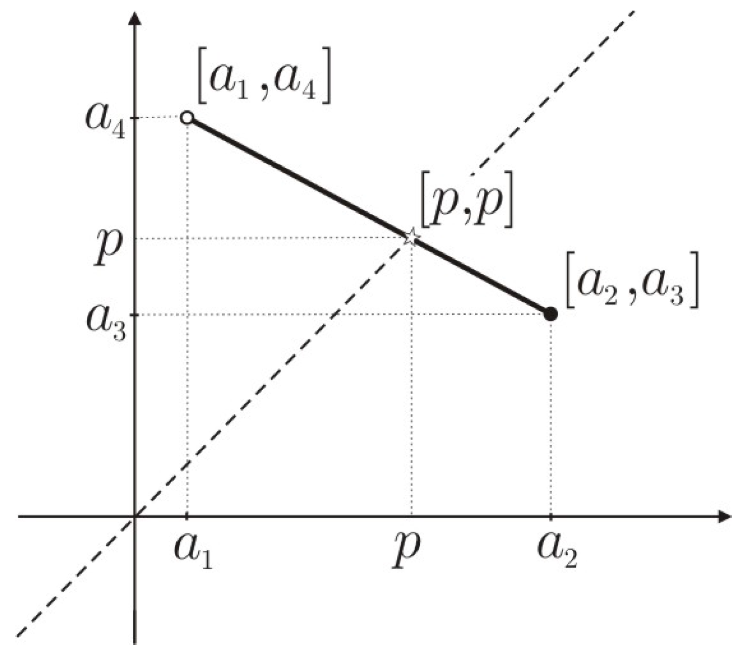
We will refer to ${\alpha }^0$ as the transition modality value of the MITFN, A. The pointwise interval $A^{{\alpha }^0}=\left[p,p\right]$ is the transition $\alpha -$cut of A, and its graphical representation is shown in Figure 4. If $A=\left(\left[a_1,a_4\right],\left[a_2,a_3\right]\right)$ is an MITFN${}_P^I$ or an MITFN${}_I^P$ and $\left[p,p\right]$ is the transition $\alpha -$cut of A, then $A_{\Delta }=\left(\left[a_1,a_4\right],\left[p,p\right]\right)$ is a modal interval triangular non-normalized fuzzy number and its modality is the same as the interval modality of the support of A, that is, if A is an MITFN${}_P^I$, then $A_{\Delta }=\left(\left[a_1,a_4\right],\left[p,p\right]\right)$ will be a proper triangular fuzzy number; while, if A is an MITFN${}_I^P$, then $A_{\Delta }=\left(\left[a_1,a_4\right],\left[p,p\right]\right)$ will be an improper triangular fuzzy number [10].

Proposition 2.

(Canonical characterization of an MITFN)

Let $A=\left(\left[a_1,a_4\right],\left[a_2,a_3\right]\right)\in T{I}^{\ast }\left(\mathbb{R}\right)$, then

• A is an MITFN${}_P^I\iff a_1\le a_3\le a_2\le a_4$;
• A is an MITFN${}_I^P\iff a_4\le a_2\le a_3\le a_1$;
• A is an MITFN${}_P^P\iff a_1\le a_2\le a_3\le a_4$;
• A is an MITFN${}_I^I\iff a_4\le a_3\le a_2\le a_1$.

Proof. 

• If A is an MITFN${}_P^I$, then $supp\left(A\right)=\left[a_1,a_4\right]$ is proper, that is, $a_1\le a_4$ and $core\left(A\right)=\left[a_2,a_3\right]$ is improper, that is, $a_3\le a_2.$
  As Definition 1 establishes $set\left(\left[a_2,a_3\right]\right)\subseteq set\left(\left[a_1,a_4\right]\right)$, in this case, $set\left(\left[a_2,a_3\right]\right)=\left[a_3,a_2\right]$ and $set\left(\left[a_1,a_4\right]\right)=\left[a_1,a_4\right]$ which means $\left[a_3,a_2\right]\subseteq$ $\left[a_1,a_4\right]$, that is $a_3\ge a_1$ and $a_2\le a_4.$
  From $a_1\le a_4,$ $a_3\le a_2,a_3\ge a_1,a_2\le a_4$, it follows that $a_1\le a_3\le a_2\le a_4.$
• If A is an MITFN${}_I^P$, $supp\left(A\right)=\left[a_1,a_4\right]$ is an improper interval, that is, $a_4\le a_1$ and $core\left(A\right)=\left[a_2,a_3\right]$ is a proper interval, that is, $a_2\le a_3.$
  As it must be that $set\left(\left[a_2,a_3\right]\right)\subseteq set\left(\left[a_1,a_4\right]\right)$ and $set\left(\left[a_2,a_3\right]\right)=\left[a_2,a_3\right],$ $set\left(\left[a_1,a_4\right]\right)=\left[a_4,a_1\right],$ so it follows that $\left[a_2,a_3\right]\subseteq$ $\left[a_4,a_1\right]$, that is, $a_2\ge a_4$ and $a_3\le a_1.$
  From $a_4\le a_1,$ $a_2\le a_3,a_2\ge a_4,a_3\le a_1$, it follows that $a_4\le a_2\le a_3\le a_1.$

The proof of both case 3 and case 4 is trivial. ☐

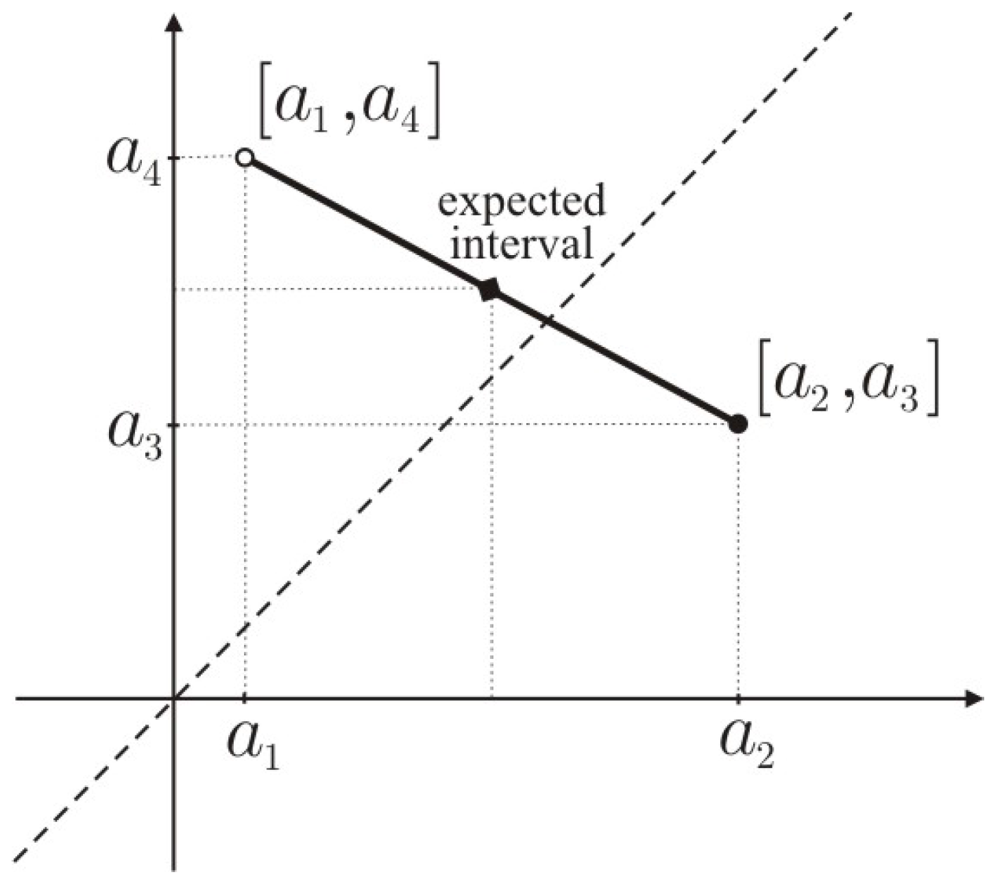
Proposition 3.

(Interval modality of the expected interval)

If $A=\left(\left[a_1,a_4\right],\left[a_2,a_3\right]\right)$ is an MITFN, then the interval modality of the expected interval is the same as the interval modality of the support of $A,$ that is:

$$mod\left(EI\left(A\right)\right)=mod\left(supp\left(A\right)\right).$$

Proof. 

The expected interval for a trapezoidal fuzzy number $A=\left(a_1,a_2,a_3,a_4\right)$ is $EI\left(A\right)=\left[\frac{a_1+a_2}{2},\frac{a_3+a_4}{2}\right].$

• If both $supp\left(A\right)$ and $core\left(A\right)$ are proper intervals, then $a_1\le a_4$ and $a_2\le a_3$ so $a_1+a_2\le a_3+a_4$ and $\left[\frac{a_1+a_2}{2},\frac{a_3+a_4}{2}\right]$ is a proper interval.
• If both $supp\left(A\right)$ and $core\left(A\right)$ are improper intervals, then $a_1\ge a_4$ and $a_2\ge a_3$ so $a_1+a_2\ge a_3+a_4$ and $\left[\frac{a_1+a_2}{2},\frac{a_3+a_4}{2}\right]$ is an improper interval.
• If $supp\left(A\right)$ is a proper interval and $core\left(A\right)$ is an improper one, then $set\left(core\left(A\right)\right)=\left[a_3,a_2\right]$ and $set\left(supp\left(A\right)\right)=\left[a_1,a_4\right]$. As $set\left(core\left(A\right)\right)\subseteq set\left(supp\left(A\right)\right),$ it holds that $a_3\ge a_1$ and $a_2\le a_4.$ Thus, $\left[\frac{a_1+a_2}{2},\frac{a_3+a_4}{2}\right]$ is a proper interval.
• If $supp\left(A\right)$ is an improper interval and $core\left(A\right)$ is a proper interval, then $set\left(core\left(A\right)\right)=\left[a_2,a_3\right]$ and $set\left(supp\left(A\right)\right)=\left[a_4,a_1\right]$. As $set\left(core\left(A\right)\right)\subseteq set\left(supp\left(A\right)\right),$ it holds that $a_2\ge a_4$ and $a_3\le a_1.$ Thus, $\left[\frac{a_1+a_2}{2},\frac{a_3+a_4}{2}\right]$ is an improper interval.

 ☐

The graphical representation of the expected interval is shown in Figure 5.

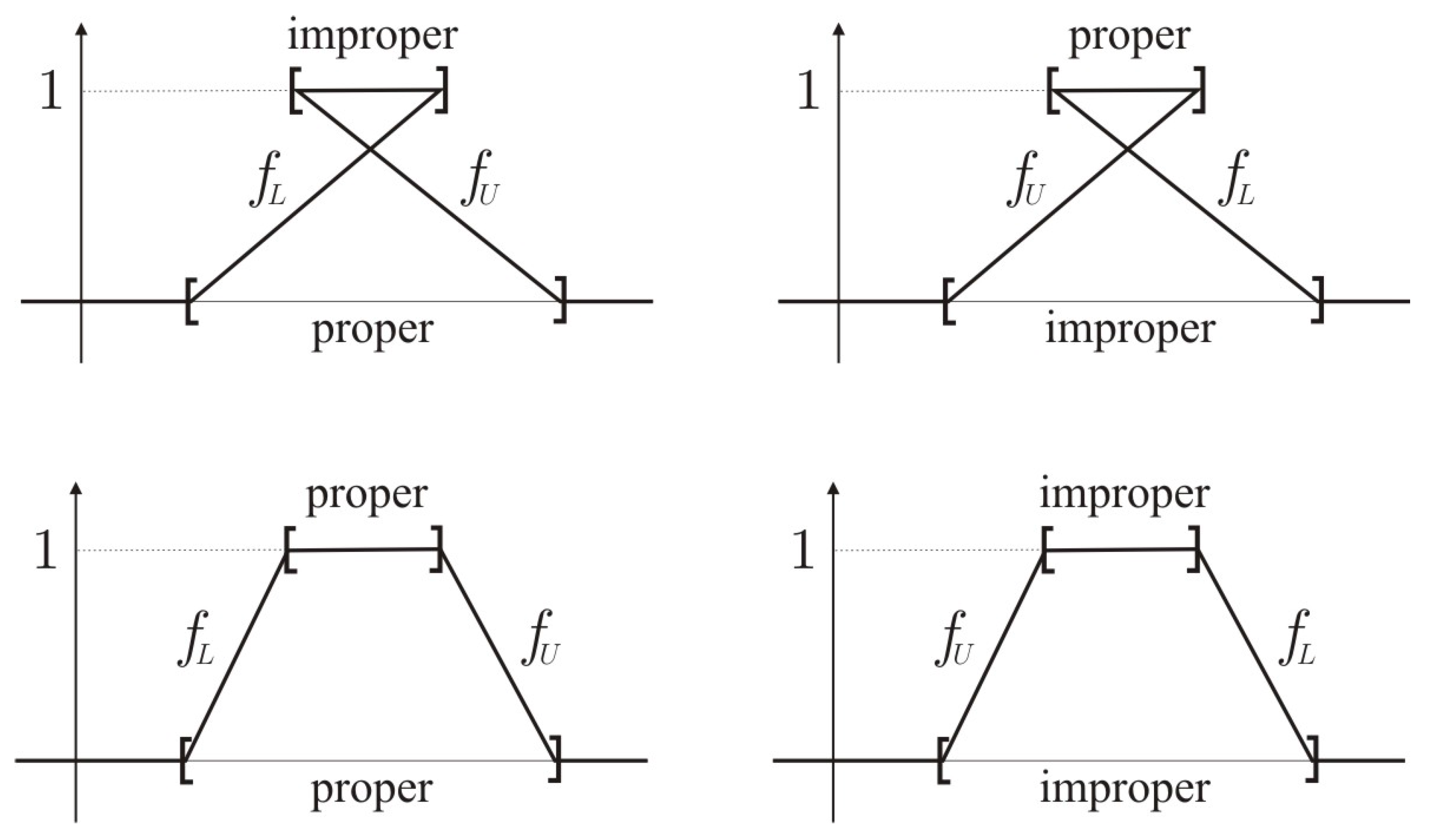
It is possible to consider the membership function of an MITFN, but it is difficult to represent improper intervals in the Cartesian plane. However, a graphical visualization of the functions $f_L$ and $f_U$ is provided in Figure 2.

Next, we will define some operators on the set of MITFNs.

Dual operator. If $A=\left(A^{\prime },Q_1,Q_2\right)\in$ $T{I}^{\ast }\left(\mathbb{R}\right)$ the dual operator on A, $dual\left(A\right)$ is defined as:

$$dual\left(A\right)=\left(A^{\prime },dual\left(Q_1\right),dual\left(Q_2\right)\right),$$

where $dual\left(Q\right)=\left\{\begin{array}{cc}\forall ,& \mathrm{if}Q=\exists ,\\ \exists ,& \mathrm{if}Q=\forall .\end{array}\right.$

We will distinguish between the dual operator of an MITFN, which we will represent by $dual\left(\right)$ and the dual operator of an interval, which we will represent by $du\left(\right).$

If $A=\left(\left[a_1,a_4\right],\left[a_2,a_3\right]\right)\in T{I}^{\ast }\left(\mathbb{R}\right)$, then $dual\left(A\right)=\left(\left[a_4,a_1\right],\left[a_3,a_2\right]\right)$. Moreover, ${\left(dual\left(A\right)\right)}^{\alpha }=du\left(A^{\alpha }\right)$ and, consequently, $supp\left(dual\left(A\right)\right)=du\left(supp\left(A\right)\right)$ and $core\left(dual\left(A\right)\right)=du\left(core\left(A\right)\right)$, that is, if $A=\left(A^0,A^1\right)$, then $dual\left(A\right)=\left(du\left(A^0\right),du\left(A^1\right)\right).$

It is obvious that if A is an MITFN${}_P^I$, then $dual\left(A\right)$ is an MITFN${}_I^P$; if A is an MITFN${}_I^P$, then $dual\left(A\right)$ is an MITFN${}_P^I$; if A is an MITFN${}_P^P$, then $dual\left(A\right)$ is an MITFN${}_I^I$; and if A is an MITFN${}_I^I$, then $dual\left(A\right)$ is an MITFN${}_P^P$.

Proper and improper operators. If $A=\left(A^{\prime },Q_1,Q_2\right)\in$ $T{I}^{\ast }\left(\mathbb{R}\right)$ we define the proper operator on $A,$ as $prop\left(A\right)=\left(A^{\prime },\exists ,\exists \right)$ and the improper operator on A as $impr\left(A\right)=\left(A^{\prime },\forall ,\forall \right)$. Using the canonical notation, if $A=\left(\left[a_1,a_4\right],\left[a_2,a_3\right]\right)$, then:

$$prop\left(A\right)=\left(\left[min\left\{a_1,a_4\right\},max\left\{a_1,a_4\right\}\right],\left[min\left\{a_2,a_3\right\},max\left\{a_2,a_3\right\}\right]\right),$$

which coincides with $set\left(A\right)$, and

$$impr\left(A\right)=\left(\left[max\left\{a_1,a_4\right\},min\left\{a_1,a_4\right\}\right],\left[max\left\{a_2,a_3\right\},min\left\{a_2,a_3\right\}\right]\right).$$

Both $prop\left(A\right)$ and $impr\left(A\right)$ are quantified trapezoidal fuzzy numbers [10].

3.1. Graphical Representation of an MITFN in the Interval Plane

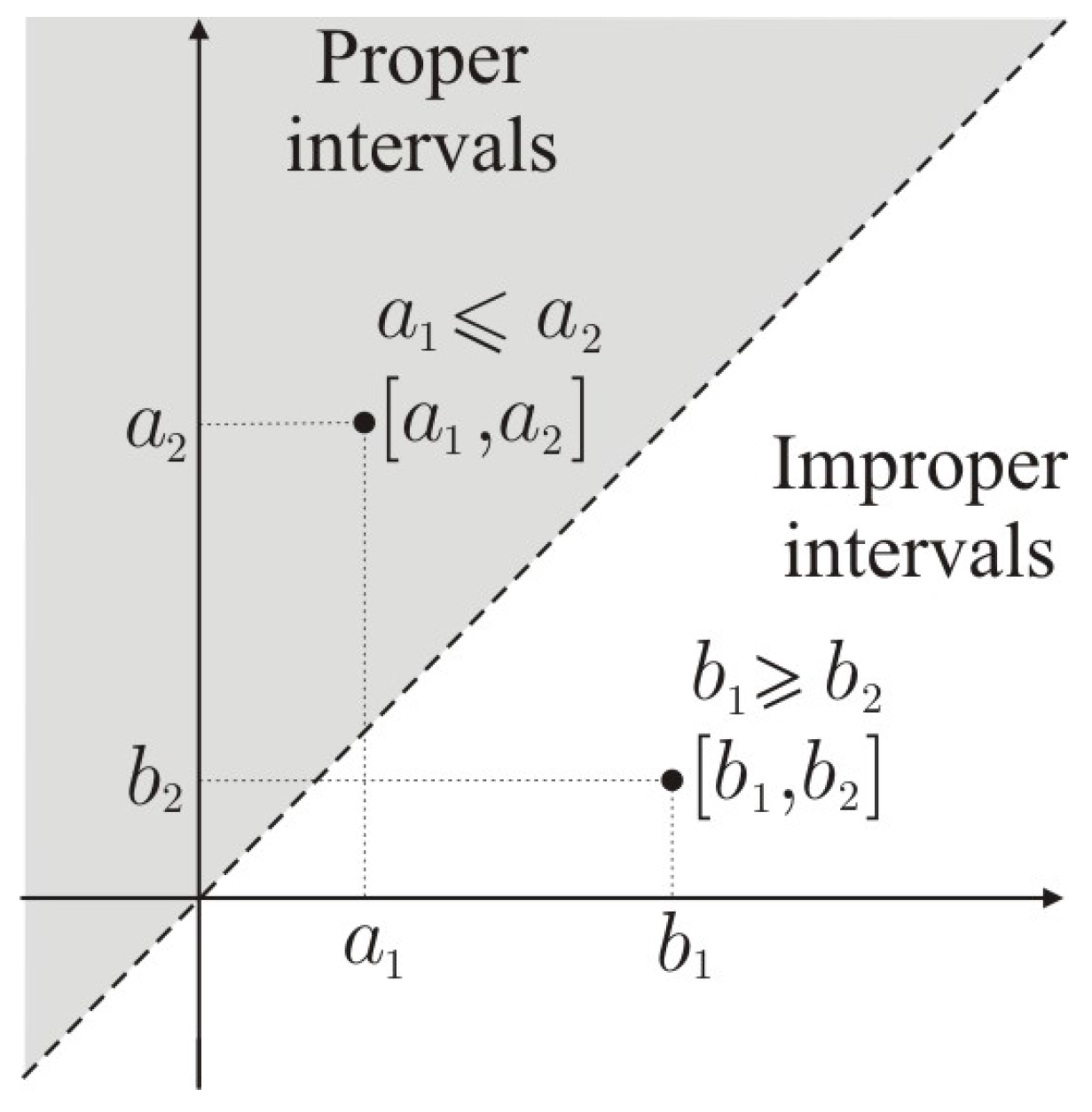
Trapezoidal fuzzy numbers, in their traditional sense, can be represented in Moore’s semiplane as decreasing segments in which the support is represented by ∘ and the core is represented by • [30].

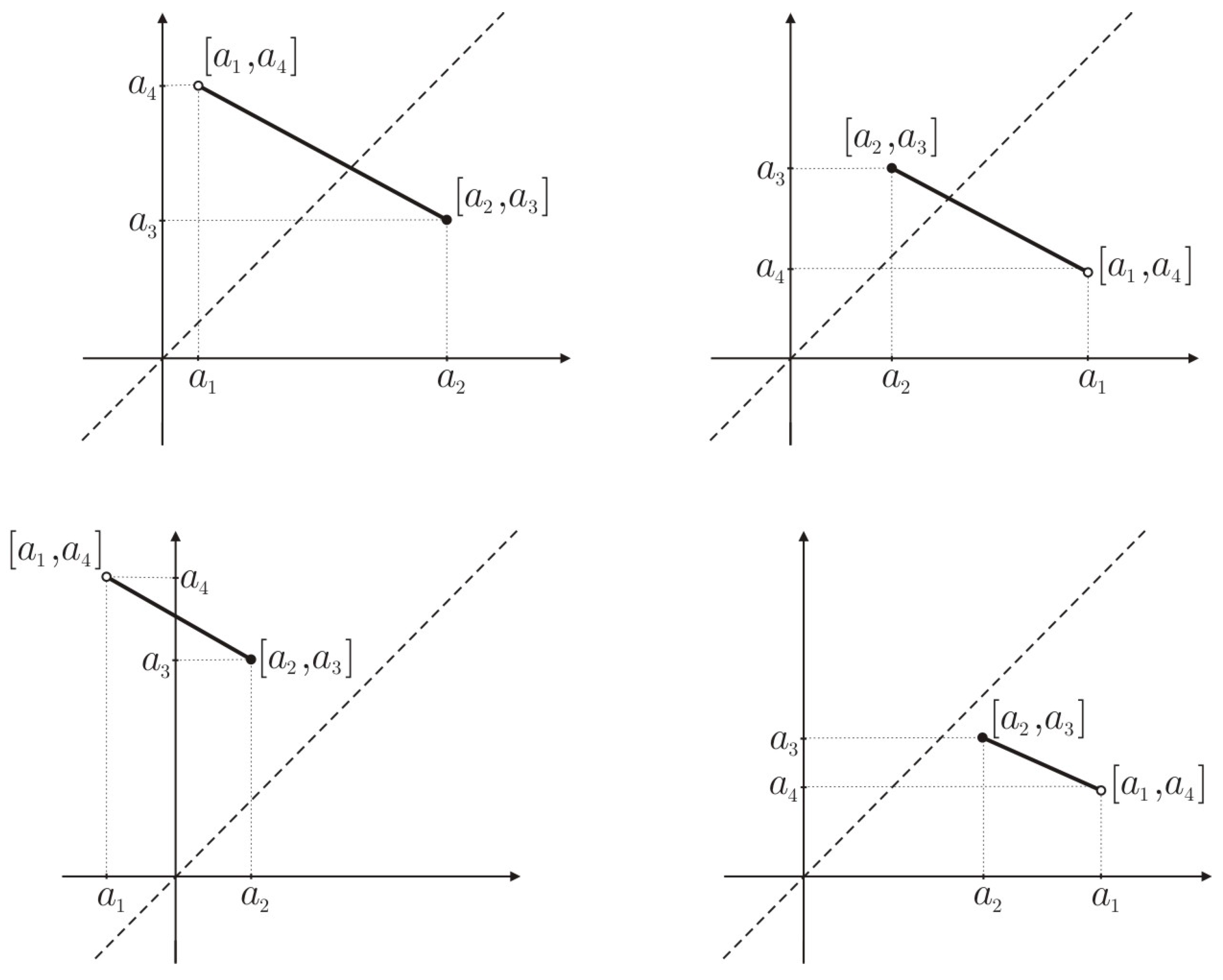
Moore’s semiplane is not detailed enough to represent an MITFN, and we must use the intervalar plane to represent them graphically. Using the same notation, that is, representing the support of an MITFN A by ∘ and representing its core by •, the segment with ends ∘ and • represents the MITFN A. The graphic representation of the four types of MITFNs, described in Definition 2, is shown in Figure 3.

The following graphical representation Figure 4 allows us to interpret the existence and uniqueness of the transition modality value easily, as well as the transition $\alpha$-cut of an MITFN${}_P^I$ or an MITFN${}_I^P$. Figure 5 is the graphic representation of the expected interval of an MITFN.

3.2. The Lattice of MITFNs

We have defined the MITFN (Definition 1) using the $\alpha$-cuts, and we will now define the inclusion relation between two MITFNs using the modal interval inclusion of the $\alpha$-cuts, that is:

$$A\subseteq B\iff \left(\forall \alpha \in \left[0,1\right]\Rightarrow A^{\alpha }\subseteq B^{\alpha }\right).$$

In the following proposition, we study the inclusion relation between two MITFNs A and B using the modalities of the support and the core of both A and B. There are 16 cases to be considered, but, using the properties of the modal interval duality, we can reduce those 16 cases to 10.

Lemma 1.

Let $A,B\in T{I}^{\ast }\left(\mathbb{R}\right)$, then:

$$A\subseteq B\iff supp\left(A\right)\subseteq supp\left(B\right)andcore\left(A\right)\subseteq core\left(B\right).$$

Proof. 

$\Rightarrow )$ As $A\subseteq B\iff \left(\forall \alpha \in \left[0,1\right]\Rightarrow A^{\alpha }\subseteq B^{\alpha }\right)$, taking $\alpha =1$ and $\alpha =0$, it follows that $supp\left(A\right)=A^0\subseteq B^0=supp\left(B\right)$ and $core\left(A\right)=A^1\subseteq B^1=core\left(B\right)$.

$\Leftarrow )$ $A=\left(\left[a_1,a_4\right],\left[a_2,a_3\right]\right)$ and $B=\left(\left[b_1,b_4\right],\left[b_2,b_3\right]\right)$.

As $\alpha \ge 0$ and $\left[a_2,a_3\right]\subseteq \left[b_2,b_3\right]\Rightarrow \alpha$ $\left[a_2,a_3\right]\subseteq \alpha \left[b_2,b_3\right].$ Moreover, as $1-\alpha \ge 0,$ $\left[a_1,a_4\right]\subseteq \left[b_1,b_4\right]$ then $\left(1-\alpha \right)$ $\left[a_1,a_4\right]\subseteq \left(1-\alpha \right)\left[b_1,b_4\right].$

Thus, $A^{\alpha }=\left(1-\alpha \right)$ $\left[a_1,a_4\right]+\alpha \left[a_2,a_3\right]\subseteq \left(1-\alpha \right)\left[b_1,b_4\right]+\alpha \left[b_2,b_3\right]=B^{\alpha }$. ☐

Proposition 4.

Given $A,B\in T{I}^{\ast }\left(\mathbb{R}\right)$, where $A=\left(A^{\prime },Q_1^A,Q_2^A\right)$ and $B=\left(B^{\prime },Q_1^B,Q_2^B\right),$ it follows that:

• If $A=\left(A^{\prime },\exists ,\exists \right)$ and $B=\left(B^{\prime },\exists ,\exists \right)$, then
  $A\subseteq B\iff set\left(supp\left(A\right)\right)\subseteq set\left(supp\left(B\right)\right)$ and $set\left(core\left(A\right)\right)\subseteq set\left(core\left(B\right)\right)$;
• If $A=\left(A^{\prime },\exists ,\exists \right)$ and $B=\left(B^{\prime },\forall ,\forall \right)$, then
  $A\subseteq B\iff A=B=\left(p,p,p,p\right)$;
• If $A=\left(A^{\prime },\exists ,\exists \right)$ and $B=\left(B^{\prime },\exists ,\forall \right)$, then
  $A\subseteq B\iff set\left(supp\left(A\right)\right)\subseteq set\left(supp\left(B\right)\right)$ and $core\left(A\right)=core\left(B\right)=\left[p,p\right]$;
• If $A=\left(A^{\prime },\exists ,\exists \right)$ and $B=\left(B^{\prime },\forall ,\exists \right)$, then
  $A\subseteq B\iff A=B=\left(p,p,p,p\right)$;
• If $A=\left(A^{\prime },\forall ,\forall \right)$ and $B=\left(B^{\prime },\exists ,\exists \right)$, then
  $A\subseteq B\iff set\left(supp\left(A\right)\right)\cap set\left(supp\left(B\right)\right)\ne \varnothing$ and $set\left(core\left(A\right)\right)\cap set\left(core\left(B\right)\right)\ne \varnothing$;
• If $A=\left(A^{\prime },\forall ,\forall \right)$ and $B=\left(B^{\prime },\exists ,\forall \right)$, then
  $A\subseteq B\iff$ $set\left(supp\left(A\right)\right)\cap set\left(supp\left(B\right)\right)\ne \varnothing$ and $set\left(core\left(A\right)\right)\supseteq set\left(core\left(B\right)\right)$;
• If $A=\left(A^{\prime },\forall ,\forall \right)$ and $B=\left(B^{\prime },\forall ,\exists \right)$, then
  $A\subseteq B\iff set\left(supp\left(A\right)\right)\supseteq set\left(supp\left(B\right)\right)$ and $set\left(core\left(A\right)\right)\cap set\left(core\left(B\right)\right)\ne \varnothing$;
• If $A=\left(A^{\prime },\exists ,\forall \right)$ and $B=\left(B^{\prime },\exists ,\forall \right)$, then
  $A\subseteq B\iff set\left(supp\left(A\right)\right)\subseteq set\left(supp\left(B\right)\right)$ and $set\left(core\left(A\right)\right)\supseteq set\left(core\left(B\right)\right)$;
• If $A=\left(A^{\prime },\exists ,\forall \right)$ and $B=\left(B^{\prime },\forall ,\exists \right)$, then
  $A\subseteq B\iff A=B=\left(p,p,p,p\right)$;
• If $A=\left(A^{\prime },\forall ,\exists \right)$ and $B=\left(B^{\prime },\exists ,\forall \right)$, then
  $A\subseteq B\iff set\left(supp\left(A\right)\right)\cap set\left(supp\left(B\right)\right)\ne \varnothing$ and $core\left(A\right)=core\left(B\right)=\left[p,p\right].$

Proof. 

As the inclusion of two modal intervals $X,Y$ conforms to the following (Gardeñes, [9]):

$$X\subseteq Y\iff \left\{\begin{array}{cc}set\left(X\right)\subseteq set\left(Y\right),& \mathrm{if}X\mathrm{and}Y\mathrm{are}\mathrm{both}\mathrm{proper},\hfill \\ set\left(Y\right)\subseteq set\left(X\right),& \mathrm{if}X\mathrm{and}Y\mathrm{are}\mathrm{both}\mathrm{improper},\hfill \\ set\left(X\right)\cap set\left(Y\right)\ne \varnothing ,& \mathrm{if}X\mathrm{is}\mathrm{improper}\mathrm{and}Y\mathrm{is}\mathrm{proper},\hfill \\ X=Y=\left[p,p\right],& \mathrm{if}X\mathrm{is}\mathrm{proper}\mathrm{and}Y\mathrm{is}\mathrm{improper}.\hfill \end{array}\right.$$

By applying Lemma 1 to the $\alpha$-cuts $A^{\alpha }$ and $B^{\alpha }$, which are modal intervals, we obtain the desired result. ☐

Notice that the following six cases:

$\left\{\left(A^{\prime },\forall ,\forall \right),\left(B^{\prime },\forall ,\forall \right)\right\}$, $\left\{\left(A^{\prime },\exists ,\forall \right),\left(B^{\prime },\forall ,\forall \right)\right\}$, $\left\{\left(A^{\prime },\exists ,\forall \right),\left(B^{\prime },\exists ,\exists \right)\right\}$,

$\left\{\left(A^{\prime },\forall ,\exists \right),\left(B^{\prime },\forall ,\exists \right)\right\}$, $\left\{\left(A^{\prime },\forall ,\exists \right),\left(B^{\prime },\exists ,\exists \right)\right\}$, $\left\{\left(A^{\prime },\forall ,\exists \right),\left(B^{\prime },\forall ,\forall \right)\right\}$, are not treated in the above Proposition 4, as they are dual cases of some of those studied, and it is possible to apply the property $A\subseteq B\iff dual\left(B\right)\subseteq dual\left(A\right).$

From the above Lemma 1, it is possible to express the inclusion relation of two MITFNs in terms of their coordinates. Thus, if $A,B\in T{I}^{\ast }\left(\mathbb{R}\right)$, $A=\left(\left[a_1,a_4\right],\left[a_2,a_3\right]\right)$ and $B=\left(\left[b_1,b_4\right],\left[b_2,b_3\right]\right)$, then:

$$A\subseteq B\iff a_1\ge b_1,a_4\le b_4,a_2\ge b_2\mathrm{and}{a}_3\le b_3.$$

Definition 3.

(Infimum and supremum)

Given $A,B,X,Y\in T{I}^{\ast }\left(\mathbb{R}\right)$,

• $inf\left\{A,B\right\}=X$ if $X\subseteq A,X\subseteq B$ and if there exists a $D\in T{I}^{\ast }\left(\mathbb{R}\right)$ such that $D\subseteq A$and $D\subseteq B$, then $D\subseteq X$;
• $sup\left\{A,B\right\}=Y$ if $A\subseteq Y,B\subseteq Y$ and if there exists a $D\in T{I}^{\ast }\left(\mathbb{R}\right)$ such that $A\subseteq D$and $B\subseteq D$, then $Y\subseteq D.$

Proposition 5.

Given $A,B\in T{I}^{\ast }\left(\mathbb{R}\right)$, let us consider $L^0=A^0\wedge B^0$ and $L^1=A^1\wedge B^1$, then

$$inf\left\{A,B\right\}=\left\{\begin{array}{cc}\left(L^0,L^1\right),& \mathrm{if}set\left(L^1\right)\subseteq set\left(L^0\right),\\ \\ \left(L^0\wedge L^1,L^1\right),& \mathrm{if}set\left(L^1\right)⊈set\left(L^0\right).\end{array}\right.$$

Proof. 

We should consider the following four cases, depending on the modalities of $L^0$ and $L^1.$

• $L^0$ and $L^1$ are proper intervals.
  As $L^0$ and $L^1$ are proper intervals, then A and B are MITFNs${}_P^P$. Thus, $A^1\subseteq A^0$ and $B^1\subseteq B^0$ so $L^1\subseteq L^0$ and as $L^1$ and $L^0$ are proper intervals, $set\left(L^1\right)\subseteq set\left(L^0\right)$. If $X=\left(L^0,L^1\right)$, then $X\subseteq A$, $X\subseteq B$ and $X\in T{I}^{\ast }\left(\mathbb{R}\right)$. Moreover, if $D\in T{I}^{\ast }\left(\mathbb{R}\right)$ conforms to $D\subseteq A$and $D\subseteq B$, then $D^0\subseteq A^0,$ $D^0\subseteq B^0$, $D^1\subseteq A^1$and $D^1\subseteq B^1$ so $D^0\subseteq A^0\wedge B^0$ and $D^1\subseteq A^1\wedge B^1$. That is, $D\subseteq X$; thus, $\left(L^0,L^1\right)=$ Inf$\left\{A,B\right\}.$
• $L^0$ is a proper interval and $L^1$ an improper interval.
  As $L^0=A^0\wedge B^0$ is a proper interval, $L^1=A^1\wedge B^1$ is an improper interval and $set\left(A^1\right)\subseteq set\left(A^0\right),$ $set\left(B^1\right)\subseteq set\left(B^0\right),$ and it follows that $L^1\subseteq L^0.$ We distinguish the following two cases according to the inclusion set of $L^1$ and $L^0$:

  (a)

  If $set\left(L^1\right)\subseteq set\left(L^0\right)$, we can proceed as in the first case.

  (b)

  If $set\left(L^1\right)⊈set\left(L^0\right)$, then let us prove that $X=\left(L^0\wedge L^1,L^1\right)$ corresponds to $inf\left\{A,B\right\}$. Notice that, if $L^1\subseteq L^0$, then $L^0\wedge L^1=L^1$; thus, $X=\left(L^1,L^1\right)$. It is obvious that $X\in T{I}^{\ast }\left(\mathbb{R}\right)$. Moreover, $X^0\subseteq A^0$ and $X^0\subseteq B^0$ as $X^0=L^1\subseteq L^0$. In a similar way, $X^1\subseteq A^1$ and $X^1\subseteq B^1$. Therefore, $X\subseteq A$ and $X\subseteq B$.

  If $D\in T{I}^{\ast }\left(\mathbb{R}\right)$ conforms to $D\subseteq A$and $D\subseteq B$, then $D^1\subseteq A^1\wedge B^1=L^1.$ Notice that, as $L^1$ is an improper interval, $D^1$ will also be an improper interval and then $set\left(L^1\right)\subseteq set\left(D^1\right)$.

  We must prove that $D^0\subseteq L^1$ and, consequently, $D\subseteq X$.

  • If $D^0$ is an improper interval, as $set\left(D^1\right)\subseteq set\left(D^0\right)$, it follows that $D^0\subseteq D^1.$ As $D^1\subseteq L^1$, then $D^0\subseteq L^1$.
  • If $D^0$ is a proper interval, as $set\left(D^1\right)\subseteq set\left(D^0\right)=D^0$ and $D^0\subseteq L^0$, it follows that $set\left(D^1\right)\subseteq L^0.$ Using the inclusion $set\left(L^1\right)\subseteq set\left(D^1\right)$, we obtain $set\left(L^1\right)\subseteq set\left(L^0\right),$ which contradicts the hypothesis $set\left(L^1\right)⊈set\left(L^0\right)$.

• $L^0$ is an improper interval and $L^1$ a proper one.
  As $L^0=A^0\wedge B^0$ is an improper interval, $L^1=A^1\wedge B^1$ is a proper interval and $set\left(A^1\right)\subseteq set\left(A^0\right),$ $set\left(B^1\right)\subseteq set\left(B^0\right)$, and it follows that $set\left(L^1\right)\subseteq set\left(L^0\right)$; thus, the demonstration follows as in the first case.
• $L^0$ and $L^1$ are improper intervals.

  (a)

  If $L^1\subseteq L^0$, then $set\left(L^0\right)\subseteq set\left(L^1\right)$. Let us prove that $X=\left(L^0\wedge L^1,L^1\right)$ corresponds to $inf\left\{A,B\right\}$. Notice that if $L^1\subseteq L^0$, then $L^0\wedge L^1=L^1$ and thus $X=\left(L^1,L^1\right)$. It is obvious that $X\in T{I}^{\ast }\left(\mathbb{R}\right)$. Moreover, $X^0\subseteq A^0$ and $X^0\subseteq B^0$ as $X^0=L^1\subseteq L^0$. In a similar way, $X^1\subseteq A^1$ and $X^1\subseteq B^1$. Therefore, $X\subseteq A$ and $X\subseteq B$.

  If $D\in T{I}^{\ast }\left(\mathbb{R}\right)$ conforms to $D\subseteq A$and $D\subseteq B$, then $D^1\subseteq A^1\wedge B^1=L^1$ and $D^0\subseteq A^0\wedge B^0=L^0$. This implies that $D^0$ and $D^1$ are improper intervals.

  Moreover, as $set\left(D^1\right)\subseteq set\left(D^0\right)$, then due to the modality of $D^0$ and $D^1$ it will be the case that $D^0\subseteq D^1$ and as $D^1\subseteq L^1$, it follows that $D^0\subseteq L^1$. Thus, $X=\left(L^0\wedge L^1,L^1\right)=inf\left\{A,B\right\}.$

  (b)

  If $L^0\subseteq L^1$, then $set\left(L^1\right)\subseteq set\left(L^0\right)$. Let us prove that $X=\left(L^0,L^1\right)$ corresponds to $inf\left\{A,B\right\}$. If $X=\left(L^0,L^1\right)$, then $X\subseteq A$, $X\subseteq B$ and $X\in T{I}^{\ast }\left(\mathbb{R}\right)$. Moreover, if $D\in T{I}^{\ast }\left(\mathbb{R}\right)$ conforms to $D\subseteq A$and $D\subseteq B$, then $D^0\subseteq A^0,$ $D^0\subseteq B^0$, $D^1\subseteq A^1$and $D^1\subseteq B^1$ so $D^0\subseteq A^0\wedge B^0$ and $D^1\subseteq A^1\wedge B^1$. That is, $D\subseteq X$; thus, $\left(L^0,L^1\right)=$ Inf$\left\{A,B\right\}.$

  (c)

  If $L^0\le L^1$ or $L^1\le L^0$, then let us prove that $X=\left(L^0\wedge L^1,L^1\right)$ corresponds to $inf\left\{A,B\right\}$. Notice that $L^0\wedge L^1\subseteq L^1$ as $L^0\wedge L^1$ and $L^1$ are improper intervals, $set\left(L^1\right)\subseteq set\left(L^0\wedge L^1\right),$ thus $X\in T{I}^{\ast }\left(\mathbb{R}\right)$ and obviously $X\subseteq A$ and $X\subseteq B$.

  If $D\in T{I}^{\ast }\left(\mathbb{R}\right)$ conforms to $D\subseteq A$and $D\subseteq B$, then $D^1\subseteq A^1\wedge B^1=L^1$ and $D^0\subseteq A^0\wedge B^0=L^0$. As $L^1$ and $L^0$ are both improper, $D^1$ and $D^0$ will also be improper intervals.

  Moreover, as $set\left(D^1\right)\subseteq set\left(D^0\right)$, then due to the modality of $D^0$ and $D^1$, it will be the case that $D^0\subseteq D^1$ and as $D^1\subseteq L^1$, it follows that $D^0\subseteq L^1$ and consequently $D^0\subseteq L^0\wedge L^1$. That is $D\subseteq X$, thus $X=\left(L^0\wedge L^1,L^1\right)=inf\left\{A,B\right\}$.

☐

Proposition 6.

Given $A,B\in T{I}^{\ast }\left(\mathbb{R}\right)$, let us consider $M^0=A^0\vee B^0$ and $M^1=A^1\vee B^1$, then:

$$sup\left\{A,B\right\}=\left\{\begin{array}{cc}\left(M^0,M^1\right),& ifset\left(M^1\right)\subseteq set\left(M^0\right),\\ \\ \left(M^0\vee M^1,M^1\right),& ifset\left(M^1\right)⊈set\left(M^0\right).\end{array}\right.$$

Proof. 

Applying modal interval properties relating duality and meet–join operators [24], that is:

$$\begin{array}{ccc}\hfill du\left(M^0\right)& =& du\left(A^0\vee B^0\right)=du\left(A^0\right)\wedge du\left(B^0\right)\hfill \\ \hfill du\left(M^1\right)& =& du\left(A^1\vee B^1\right)=du\left(A^1\right)\wedge du\left(B^1\right)\hfill \end{array}$$

and

$$sup\left\{A,B\right\}=dual\left(inf\left\{dual\left(A\right),dual\left(B\right)\right\}\right)$$

Let $L^0$ be $L^0=du\left(A^0\right)\wedge du\left(B^0\right)$. As $set\left(L^0\right)=set\left(du\left(L^0\right)\right)$, then

$$set\left(L^0\right)=set\left(du\left(du\left(A^0\right)\wedge du\left(B^0\right)\right)\right)=set\left(A^0\vee B^0\right).$$

In the same way, if $L^1=du\left(A^1\right)\wedge du\left(B^1\right)$, then $set\left(L^1\right)=set\left(A^1\vee B^1\right).$

When we calculate Inf$\left\{dual\left(A\right),dual\left(B\right)\right\},$ we should consider:

• If $set\left(L^1\right)\subseteq set\left(L^0\right)$, then $set\left(M^1\right)\subseteq set\left(M^0\right)$ and so:

  $$\begin{array}{ccc}\hfill sup\left\{A,B\right\}& =& dual\left(du\left(A^0\right)\wedge du\left(B^0\right),du\left(A^1\right)\wedge du\left(B^1\right)\right)\hfill \\ & =& \left(du\left(du\left(A^0\right)\wedge du\left(B^0\right)\right),du\left(du\left(A^1\right)\wedge du\left(B^1\right)\right)\right)\hfill \\ & =& \left(A^0\vee B^0,A^1\vee B^1\right)=\left(M^0,M^1\right).\hfill \end{array}$$
• If $set\left(L^1\right)⊈set\left(L^0\right)$, then

  $$\begin{array}{ccc}\hfill sup\left\{A,B\right\}& =& dual\left(du\left(A^0\right)\wedge du\left(B^0\right)\wedge du\left(A^1\right)\wedge du\left(B^1\right),du\left(A^1\right)\wedge du\left(B^1\right)\right)\hfill \\ & =& \left(du\left(du\left(A^0\right)\wedge du\left(B^0\right)\right),du\left(du\left(A^1\right)\wedge du\left(B^1\right)\right)\right)\hfill \\ & =& \left(A^0\vee B^0\vee A^1\vee B^1,A^1\vee B^1\right)=\left(M^0\vee M^1,M^1\right).\hfill \end{array}$$

☐

4. Interpretability of the Calculations

Definition 4.

(Modal extension of a real function)

Let $f:{\mathbb{R}}^n⟶\mathbb{R}$ be a real continuous function. We represent the modal interval trapezoidal fuzzy extension associated with f by $TI{f}^{\ast },$ and we define it over $\left(X_1,\dots ,X_n\right)\in {\left(T{I}^{\ast }\left(\mathbb{R}\right)\right)}^n$ using the interval extension $f^{\ast }$ (see Sainz [24,31]) over the $\alpha -$cuts of the MITFNs $\left(X_1^{\alpha },\dots ,X_n^{\alpha }\right):$

$$TI{f}^{\ast }\left(X_1,\dots ,X_n\right)=\left\{f^{\ast }\left(X_1^{\alpha },\dots ,X_n^{\alpha }\right),\alpha \in \left[0,1\right]\right\}.$$

As the $\alpha$-cuts are modal intervals, we can express this modal interval trapezoidal fuzzy extension using the meet and join operators, and splitting the components of $X_1^{\alpha },\dots ,X_n^{\alpha }$ into the proper ones: $X_{j_P}^{\alpha }$ and the improper ones: $X_{j_I}^{\alpha }$

$$TI{f}^{\ast }\left(X_1,\dots ,X_n\right)=\left\{\underset{x_{j_p}\in set\left(X_{j_P}^{\alpha }\right)}{\vee }\underset{x_{j_i}\in set\left(X_{j_I}^{\alpha }\right)}{\wedge }\left[f\left(x_{j_p},x_{j_i}\right),f\left(x_{j_p},x_{j_i}\right)\right],\alpha \in \left[0,1\right]\right\},$$

which is equivalent to

$$\begin{array}{cc}\hfill TI{f}^{\ast }& \left(X_1,\dots ,X_n\right)=\hfill \\ & =\left\{\left[\underset{x_{j_p}\in set\left(X_{j_P}^{\alpha }\right)}{min}\underset{x_{j_i}\in set\left(X_{j_I}^{\alpha }\right)}{max}f\left(x_{j_p},x_{j_i}\right),\underset{x_{j_p}\in set\left(X_{j_P}^{\alpha }\right)}{max}\underset{x_{j_i}\in set\left(X_{j_I}^{\alpha }\right)}{min}f\left(x_{j_p},x_{j_i}\right)\right],\alpha \in \left[0,1\right]\right\}.\hfill \end{array}$$

Proposition 7.

(Inclusivity of the modal extension)

If $TI{f}^{\ast }$ is the modal extension of a real continuous function $f:{\mathbb{R}}^n⟶\mathbb{R}$, given $X_1,\dots ,X_n,Y_1,\dots ,Y_n\in T{I}^{\ast }\left(\mathbb{R}\right)$ such that $\forall i\in \left\{1,\dots ,n\right\}{X}_i\subseteq Y_i$, then:

$$TI{f}^{\ast }\left(X_1,\dots ,X_n\right)\subseteq TI{f}^{\ast }\left(Y_1,\dots ,Y_n\right).$$

Proof. 

We can express the inclusion of MITFNs by using the inclusion of the $\alpha$-cuts, that is $X_i\subseteq Y_i\iff \alpha \in \left[0,1\right],X_i^{\alpha }\subseteq Y_i^{\alpha }$, as the interval extension $f^{\ast }$ is inclusive ([24] [Theorem 3.2.4]).

$${\left(TI{f}^{\ast }\left(X_1,\dots ,X_n\right)\right)}^{\alpha }=f^{\ast }\left(X_1^{\alpha },\dots ,X_n^{\alpha }\right)\subseteq f^{\ast }\left(Y_1^{\alpha },\dots ,Y_n^{\alpha }\right)={\left(TI{f}^{\ast }\left(Y_1,\dots ,Y_n\right)\right)}^{\alpha }.$$

☐

Given a rational real continuous function f, if $X_1^{\alpha },\dots ,X_n^{\alpha }$ are the $\alpha$-cuts of the classical trapezoidal fuzzy numbers $X_1,\dots ,X_n$, then $\forall \alpha \in \left[0,1\right]$, and the interval extension that we represent by $F\left(X_1^{\alpha },\dots ,X_n^{\alpha }\right)=Y^{\alpha }$ associated with f can be interpreted as:

$$\left(\forall x_1\in X_1^{\alpha }\right)\cdots \left(\forall x_n\in X_n^{\alpha }\right)\left(\exists y\in Y^{\alpha }\right)\mathrm{and}f\left(x_1,\dots ,x_n\right)=y$$

(1)

or also as:

$$\left(\forall y\in Y^{\alpha }\right)\left(\exists x_1\in X_1^{\alpha }\right)\cdots \left(\exists x_n\in X_n^{\alpha }\right)\mathrm{and}f\left(x_1,\dots ,x_n\right)=y$$

(2)

because f is a continuous function and the value $Y^{\alpha }$ corresponds to:

$$\left[\underset{x_j\in X_j^{\alpha }}{min}f\left(x_1,\dots ,x_n\right),\underset{x_j\in X_j^{\alpha }}{max}f\left(x_1,\dots ,x_n\right)\right].$$

(3)

In most of the cases, $\forall \alpha \in \left[0,1\right],$ the exact values $Y^{\alpha }=F\left(X_1^{\alpha },\dots ,X_n^{\alpha }\right)$ that define the fuzzy number $Y=\left\{Y^{\alpha },\alpha \in \left[0,1\right]\right\}$ are difficult to calculate. This is the reason why we often replace every rational operator in the function f by its corresponding intervalar operator. The result obtained with this replacement is not the same interval $Y^{\alpha }$, but an interval $Z^{\alpha }$ which conforms to:

$$F\left(X_1^{\alpha },\dots ,X_n^{\alpha }\right)=Y^{\alpha }\subseteq Z^{\alpha }.$$

However, the only valid semantic application to this last calculus will be the interpretation given in Equation (1)

$$\left(\forall x_1\in X_1^{\alpha }\right)\cdots \left(\forall x_n\in X_n^{\alpha }\right)\left(\exists z\in Z^{\alpha }\right)\mathrm{and}f\left(x_1,\dots ,x_n\right)=z$$

and the semantic expressed in Equation (2) will not be applicable to this last calculus $F\left(X_1^{\alpha },\dots ,X_n^{\alpha }\right)\subseteq Z^{\alpha }$.

Theorem 1.

(Interpretability theorem)

Let $TI{f}^{\ast }:{\left(T{I}^{\ast }\left(\mathbb{R}\right)\right)}^n⟶T{I}^{\ast }\left(\mathbb{R}\right)$be the ∗-extension of a real continuous function $f:{\mathbb{R}}^n⟶\mathbb{R}$, and let $X=\left(X_1,\dots ,X_n\right)$ be a vector of MITFNs sorted by their modality, that is:

$$X=(\underset{P-P}{\underbrace{A_1,\dots ,A_i}},\underset{I-I}{\underbrace{B_1,\dots ,B_j}},\underset{P-I}{\underbrace{C_1,\dots ,C_k}},\underset{I-P}{\underbrace{D_1,\dots ,D_l}}),$$

where $i+j+k+l=n.$

If $Z=\left(Z^{\prime },Q_1,Q_2\right)\in T{I}^{\ast }\left(\mathbb{R}\right)$ conforms to $TI{f}^{\ast }\left(X_1,\dots ,X_n\right)\subseteq Z$ and we consider ${\gamma }_q^0,$ ${\delta }_r^0$ and ${\alpha }_z^0$ the transition modality values of the MITFNs $C_q,D_r$ and Z, respectively, then, given $\alpha \in \left[0,1\right],$ it holds that:

$\left(\forall \left(a_1,\dots ,a_i\right)\in set{\left(A_1,\dots ,A_i\right)}^{\alpha }\right)\left(\forall \left(c_{k_1},\dots ,c_{k_{\xi }}\right)\in set{\left(C_{k_1},\dots ,C_{k_{\xi }}\right)}^{\alpha }\right)$

$\left(\forall \left(d_{l_1},\dots ,d_{l_{\varphi }}\right)\in set{\left(D_{l_1},\dots ,D_{l\varphi }\right)}^{\alpha }\right)$

$\left(Qz\in set\left(Z^{\alpha }\right)\right)\left(\exists \left(b_1,\dots ,b_j\right)\in set{\left(B_1,\dots ,B_j\right)}^{\alpha }\right)$

$\left(\exists \left(c_{{\tilde{k}}_1},\dots ,c_{{\tilde{k}}_{\mu }}\right)\in set{\left(C_{{\tilde{k}}_1},\dots ,C_{{\tilde{k}}_{\mu }}\right)}^{\alpha }\right)$

$\left(\exists \left(d_{{\tilde{l}}_1},\dots ,d_{{\tilde{l}}_{\tau }}\right)\in set{\left(D_{{\tilde{l}}_1},\dots ,D_{{\tilde{l}}_{\tau }}\right)}^{\alpha }\right)$ such that:

$$z=f\left(a_1,\dots ,a_i,b_1,\dots ,b_j,c_1,\dots ,c_k,d_1,\dots ,d_l\right),$$

where ${\left(C_{k_1},\dots ,C_{k_{\xi }}\right)}^{\alpha }$ are the α-cuts of $C_1,\dots ,C_k$ whose interval modality is proper, ${\left(C_{{\tilde{k}}_1},\dots ,C_{{\tilde{k}}_{\mu }}\right)}^{\alpha }$ are the α-cuts of $C_1,\dots ,C_k$ whose interval modality is improper, ${\left(D_{l_1},\dots ,D_{l\varphi }\right)}^{\alpha }$ are the α-cuts of $D_1,\dots ,D_l$ whose interval modality is proper and ${\left(D_{{\tilde{l}}_1},\dots ,D_{{\tilde{l}}_{\tau }}\right)}^{\alpha }$ are the α-cuts of $D_1,\dots ,D_l$ whose interval modality is improper, and $Q=Q_1$ if $\alpha \le {\alpha }_z^0$ or $Q=Q_2$ if $\alpha >{\alpha }_z^0$.

Moreover,

$$\begin{array}{ccc}\hfill \left\{c_{k_1},\dots ,c_{k_{\xi }},c_{{\tilde{k}}_1},\dots ,c_{{\tilde{k}}_{\mu }}\right\}& =& \left\{c_1,\dots ,c_k\right\},\hfill \\ \hfill \left\{d_{l_1},\dots ,d_{l_{\varphi }},d_{{\tilde{l}}_1},\dots ,d_{{\tilde{l}}_{\tau }}\right\}& =& \left\{d_1,\dots ,d_l\right\},\hfill \end{array}$$

although the elements within these sets are not ordered in the same way.

Proof. 

The interval semantic theorem (Sainz [24]), states that if $f^{\ast }$ is the ∗-semantic extension of a real function f, and X is a vector of modal intervals expressed as $X=\left(X_P,X_I\right),$ where $X_P$ are the proper components of X and $X_I$ are the improper components of X, if $\left(Y,Q\right)\in I^{\ast }\left(\mathbb{R}\right)$ is such that $f^{\ast }\left(X_P,X_I\right)\subseteq Y$, then:

$$\left(\forall x_p\in set\left(X_P\right)\right)\left(Qy\in set\left(Y\right)\right)\left(\exists x_i\in set\left(X_I\right)\right)\mathrm{such}\mathrm{that}y=f\left(x_p,x_i\right).$$

We will now apply this semantic theorem to the $\alpha$-cuts of:

$$X=(\underset{P-P}{\underbrace{A_1,\dots ,A_i}},\underset{I-I}{\underbrace{B_1,\dots ,B_j}},\underset{P-I}{\underbrace{C_1,\dots ,C_k}},\underset{I-P}{\underbrace{D_1,\dots ,D_l}}).$$

The modality of the $\alpha$-cuts $\left(A_1^{\alpha },\dots ,A_i^{\alpha }\right)$ is always proper and the modality of the $\alpha$-cuts $\left(B_1^{\alpha },\dots ,B_j^{\alpha }\right)$ is always improper.

Let $\Omega$ be the set $\Omega ={\left\{{\gamma }_q^0,{\delta }_r^0\right\}}_{\begin{array}{c}q\in \left\{1,\dots ,k\right\}\\ r\in \left\{1,\dots ,l\right\}\end{array}}\cup \left\{{\alpha }_z^0\right\}$. Above this set $\Omega$ we define inductively

$${\theta }_1=min\Omega ,{\theta }_m=min\Omega \setminus \underset{s=1}{\stackrel{m-1}{\cup }}\left\{{\theta }_s\right\},{\theta }_{k+l+1}=1.$$

Then, given $\alpha \in \left[0,1\right]$, there will exist $p\in \left\{1,\dots ,k+l\right\}$ such that $\alpha \in \left[{\theta }_p,{\theta }_{p+1}\right].$ For this value, we must consider the modality of the $\alpha$-cuts $C_1^{\alpha },\dots ,C_k^{\alpha }$ and $D_1^{\alpha },\dots ,D_l^{\alpha }$, as some of these modalities have changed with regard to the modalities of the zero-cuts $C_1^0,\dots ,C_k^0,$ $D_1^0,\dots ,D_l^0$.

Thus, for this given $\alpha$, there will be $C_{k_1},\dots ,C_{k_{\xi }}\in \left\{C_1,\dots ,C_k\right\}$ in which the interval modality of their $\alpha$-cuts is proper, and there will be $C_{{\tilde{k}}_1},\dots ,C_{{\tilde{k}}_{\mu }}\in \left\{C_1,\dots ,C_k\right\}$ in which the interval modality of their $\alpha$-cuts is improper. At the same time, there will exist $D_{l_1},\dots ,D_{l\varphi }\in \left\{D_1,\dots ,D_l\right\}$ in which the interval modality of their $\alpha$-cuts is proper and $D_{{\tilde{l}}_1},\dots ,D_{{\tilde{l}}_{\tau }}$ in which the interval modality of their $\alpha$-cuts is improper. The interval modality of $Z^{\alpha }$ will be $Q_1$ if $\alpha \le {\alpha }_z^0$ and $Q_2$ if $\alpha >{\alpha }_z^0$. ☐

Corollary 1.

Under the above conditions of Theorem 1, if $\alpha \in \left[0,min\Omega \right]$, then:

$\left(\forall \left(a_1,\dots ,a_i\right)\in set{\left(A_1,\dots ,A_i\right)}^{\alpha }\right)\left(\forall \left(c_1,\dots ,c_k\right)\in set{\left(C_1,\dots ,C_k\right)}^{\alpha }\right)$

$\left(Q_{1}z\in set\left(Z^{\alpha }\right)\right)\left(\exists \left(b_1,\dots ,b_j\right)\in set{\left(B_1,\dots ,B_j\right)}^{\alpha }\right)$

$\left(\exists \left(d_1,\dots ,d_l\right)\in set{\left(D_1,\dots ,D_l\right)}^{\alpha }\right)$ such that

$$z=f\left(a_1,\dots ,a_i,b_1,\dots ,b_j,c_1,\dots ,c_k,d_1,\dots ,d_l\right).$$

Corollary 2.

Under the above conditions of Theorem 1, if $\alpha \in \left[max\Omega ,1\right]$, then:

$\left(\forall \left(a_1,\dots ,a_i\right)\in set{\left(A_1,\dots ,A_i\right)}^{\alpha }\right)\left(\forall \left(d_1,\dots ,d_l\right)\in set{\left(D_1,\dots ,D_l\right)}^{\alpha }\right)$

$\left(Q_{2}z\in set\left(Z^{\alpha }\right)\right)\left(\exists \left(b_1,\dots ,b_j\right)\in set{\left(B_1,\dots ,B_j\right)}^{\alpha }\right)$

$\left(\exists \left(c_1,\dots ,c_k\right)\in set{\left(C_1,\dots ,C_k\right)}^{\alpha }\right)$ such that

$$z=f\left(a_1,\dots ,a_i,b_1,\dots ,b_j,c_1,\dots ,c_k,d_1,\dots ,d_l\right).$$

Definition 5.

Let ⊙ be a binary real rational operator. Given $A,B\in T{I}^{\ast }\left({\mathbb{R}}^n\right)$: the extension of the operator ⊙ above the MITFNs A and B is represented by ⊗ and defined using the α-cuts of A and B as

$${\left(A\otimes B\right)}^{\alpha }=A^{\alpha }\odot B^{\alpha }.$$

Definition 6.

Let ⊙ be a binary real rational operator, and ⊗ its extension above the MITFNs. Given $A,B\in T{I}^{\ast }\left({\mathbb{R}}^n\right)$ if C is an MITFN, C is said to be interpretability compatible with the exact value $A\otimes B$ if $A\otimes B\subseteq C$.

Often, the result of calculating $\left\{{\left(A\otimes B\right)}^{\alpha },\alpha \in \left[0,1\right]\right\}=\left\{A^{\alpha }\odot B^{\alpha },\alpha \in \left[0,1\right]\right\}$ will not be an MITFN. There are some situations that clearly reflect this, such as the multiplication, the quotient and rounding results. This situation is well known when working with trapezoidal fuzzy numbers, in which not all the rational operators are internal operators. To preserve the inclusion expressed in the above Theorem 1, that is, $TI{f}^{\ast }\left(X_1,\dots ,X_n\right)\subseteq Z$, we will have to find $Z\in T{I}^{\ast }\left(\mathbb{R}\right)$ such that $TI{f}^{\ast }\left(X_1,\dots ,X_n\right)\subseteq Z$.

The extension of a rational real operator ⊙ above two MITFNs A and B is always interpretability compatible with the calculation of $A\otimes B$ as the intervalar extension above the $\alpha$-cuts $A^{\alpha }$ and $B^{\alpha }$ is always inclusive.

Sometimes, rounding results do not constitute a very important subject. However, if we center our study on the interpretability of the calculus, then when we evaluate $A\otimes B$ we must find a modal trapezoidal fuzzy number C such that C is interpretability compatible with $A\otimes B$.

We have just mentioned Equation (3) above, the difficulty of calculating the exact value

$$\left[\underset{x_j\in X_j^{\alpha }}{min}f\left(x_1,\dots ,x_n\right),\underset{x_j\in X_j^{\alpha }}{max}f\left(x_1,\dots ,x_n\right)\right]$$

of a rational real function f. The modal extension $TI{f}^{\ast }\left(X_1,\dots ,X_n\right)$ of the real continuous function f is even more difficult to evaluate. Thus, instead of calculating the modal extension $TI{f}^{\ast }\left(X_1,\dots ,X_n\right)$, we will evaluate a new function obtained by replacing every rational real operator in f by its corresponding operator above MITFNs. Since, on many occasions, the result of calculating these rational operators will not be an MITFN, this result will be transformed into an MITFN that is interpretability compatible with the exact result.

What we have laid out leads us to evaluate an MITFN Z that contains the exact value. Of course, this is too general and we should impose some other conditions.

Many methods to convert a non-trapezoidal fuzzy number to a trapezoidal one have been studied. Many researches have studied how to find a fuzzy number that is the nearest to a non-trapezoidal fuzzy number, which is related to the approximation of fuzzy numbers under different points of view.

Abbasbandy and Asady [32] used the metric distance between two fuzzy numbers to introduce a trapezoidal approximation. Other research such as Grzegorzewski and Mrówka [33], and Grzegorzewski [34] and Yeh [35,36] studied a nearest trapezoidal approximation preserving the expected interval.

Veerani et al. [37] proposed a method to convert any fuzzy number to the nearest symmetric trapezoidal fuzzy number approximation also preserving the expected interval.

Preserving ambiguity, value and width, Ban, Coroianu and Khastan [38] developed a general method to study the L-R approximations of fuzzy numbers. In addition, some methods for ranking fuzzy numbers using distances have been developed [39,40], but none of those trapezoidal approximations is useful to us because, although they preserve certain properties, they do not impose preservation of inclusivity and so they are not valid for semantic interpretations.

When possible, we will apply the optimal external inclusion introduced by Wagen [41], although, in some special cases, it may be necessary to add some further conditions, referring to the inclusion of the core of the result.

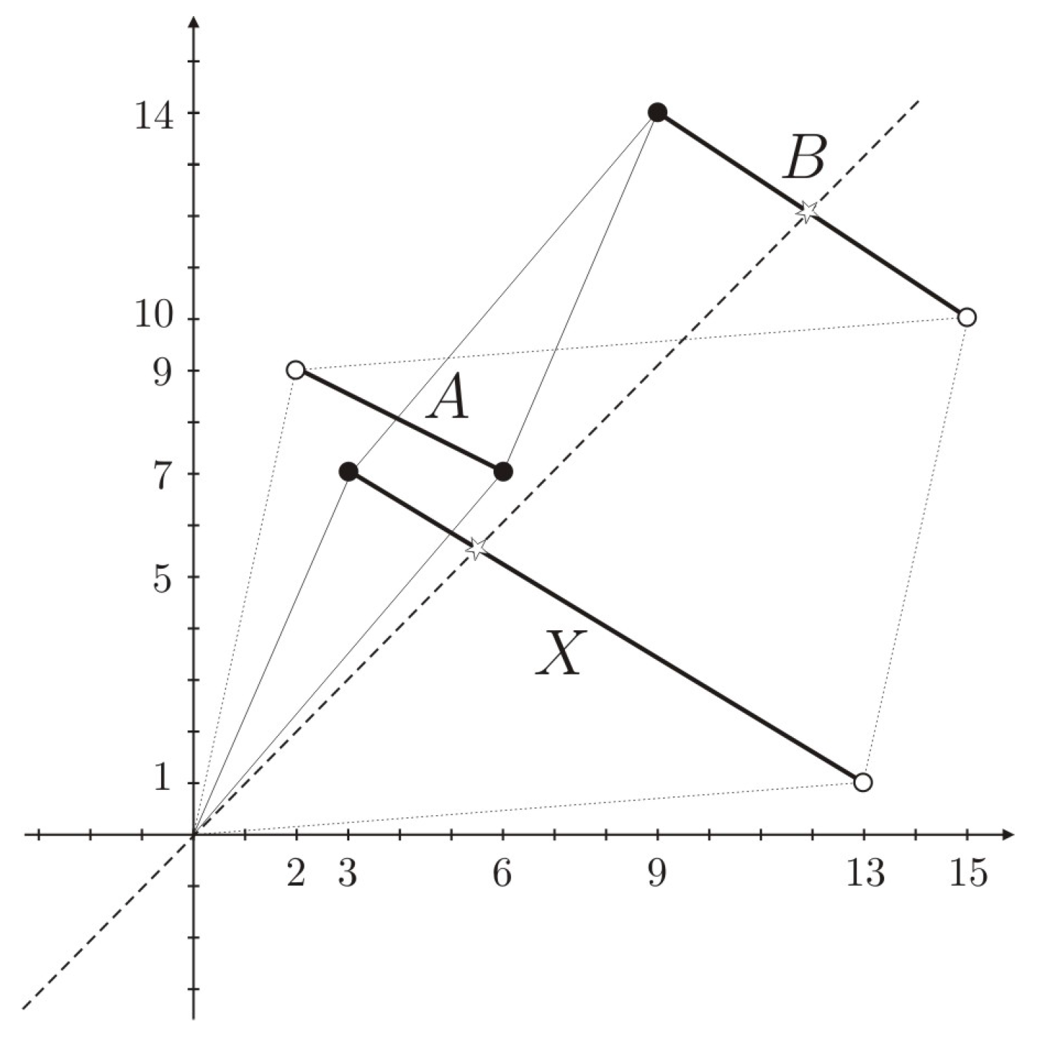
Example 1.

The fuzzy trapezoidal equation $A+X=B$ whose solution is $X=B-dual\left(A\right)$ does not always have a solution in the classical sense. However, using MITFNs, many of these equations not only have a solution, but the solution can be semantically interpreted as well.

Let us take the MITFN $A=\left(\left[0,20\right],\left[7,12\right]\right)$ and $B=\left(\left[1,30\right],\left[15,17\right]\right)$. Both A and B are proper trapezoidal fuzzy numbers, that is, trapezoidal fuzzy numbers in the classical sense. The solution of the equation

$$\left(\left[0,20\right],\left[7,12\right]\right)+X=\left(\left[1,30\right],\left[15,17\right]\right)$$

is

$$X=\left(\left[1,30\right],\left[15,17\right]\right)-dual\left(\left[0,20\right],\left[7,12\right]\right)=\left(\left[1,10\right],\left[8,5\right]\right).$$

However, $X=\left(\left[1,10\right],\left[8,5\right]\right)$ is an MITFN${}_P^I$ whose transition modality value is ${\alpha }_X^0=\frac{3}{4}.$

Thus, the interpretation is:

• $\forall \alpha \in \left[0,\frac{3}{4}\right]\left(\forall a\in set\left(A^{\alpha }\right)\right)\left(\forall x\in set\left(X^{\alpha }\right)\right)\left(\exists b\in set\left(B^{\alpha }\right)\right)$$a+x=b;$
• $\forall \alpha \in \left[\frac{3}{4},1\right]\left(\forall a\in set\left(A^{\alpha }\right)\right)\left(\exists b\in set\left(B^{\alpha }\right)\right)\left(\exists x\in set\left(X^{\alpha }\right)\right)$$a+x=b.$

Next, let us consider the fuzzy equation $A+X=B$, where A is the MITFN${}_P^P$, $A=\left(\left[2,9\right],\left[6,7\right]\right)$ and B is the MITFN${}_I^P$, $B=\left(\left[15,10\right],\left[9,14\right]\right).$ The solution for X is:

$$X=B-dual\left(A\right)=\left(\left[15,10\right],\left[9,14\right]\right)-dual\left(\left[2,9\right],\left[6,7\right]\right)=\left(\left[13,1\right],\left[3,7\right]\right),$$

which is an MITFN${}_I^P$ (see Figure 6). The transition modality value for X is ${\alpha }_X^0=\frac{3}{4}=0.75$ and the transition modality value for B is ${\alpha }_B^0=\frac{1}{2}=0.5$; thus, the interpretation of the calculus $A+X=B$ is:

• $\forall \alpha \in \left[0,0.5\right]\left(\forall a\in set\left(A^{\alpha }\right)\right)\left(\forall b\in set\left(B^{\alpha }\right)\right)\left(\exists x\in set\left(X^{\alpha }\right)\right)$$a+x=b;$
• $\forall \alpha \in \left[0.5,0.75\right]\left(\forall a\in set\left(A^{\alpha }\right)\right)\left(\exists b\in set\left(B^{\alpha }\right)\right)\left(\exists x\in set\left(X^{\alpha }\right)\right)$$a+x=b;$
• $\forall \alpha \in \left[0.75,1\right]\left(\forall a\in set\left(A^{\alpha }\right)\right)\left(\forall x\in set\left(X^{\alpha }\right)\right)\left(\exists b\in set\left(B^{\alpha }\right)\right)$$a+x=b.$

5. Conclusions

In this paper, we have used the lattice structure of modal intervals to develop the lattice completion of trapezoidal fuzzy numbers, with regard to the inclusion relation. We have named the set obtained with this completion MITFNs. The elements of this new set have been defined allowing that their $\alpha$-cuts can be modal intervals and also allowing that the support modality and the core modality are not the same. This reticular completion has not simply been left in a theoretical study of the inclusion relationship between modal trapezoidal fuzzy numbers, but the calculation of the extensions of real continuous functions has also been addressed.

Moreover, we have not simply focused on the calculation of the real extensions on MITFNs, but we have also used the semantic theorem of modal interval analysis so as to interpret the calculus to the $\alpha$-cuts of the extensions. We are certain that knowing the meaning of a calculation is even more important than the calculation itself.

With the study presented in this paper, we have provided a new tool for fuzzy numbers. We have introduced an extension of traditional trapezoidal fuzzy numbers and we have solved a problem that had no solution in the set of traditional trapezoidal fuzzy numbers, while also providing the semantic interpretation of the result obtained.

Our future lines of research are twofold; on the one hand, further theoretical research will be conducted, and, on the other, some practical applications of our theoretical studies will be developed.

Regarding theoretical studies, we believe it is interesting to look for and implement algorithms that allow us to obtain a good inclusive approach to the semantic extension $TI{f}^{\ast }$. Thus, we would reduce the typical enlargement of the interval results. This research should be supplemented with the study of optimality in the calculus of rational functions, understanding that optimality, in the sense of studying when a result obtained by replacing each of the rational operators in the real function f by the corresponding fuzzy operator, is the best possible result with regard to the inclusion relationship.

From an applied perspective, the application of MITFNs to the field of MultiCriteria Decision Making (MCDM) is also worth exploring, as there are many methods related to multicriteria analysis that use trapezoidal fuzzy numbers that could be extended to the MITFNs. Among these methods, we will pay special attention to the following: the CODAS method (Combinative Distance-based Assessment) [42], QUALIFLEX method (QUALItative FLEXible) [43], ELECTRE method (ELimination Et Choix Traduisant la REalité) [44,45], VIKOR method (VlseKriterijumska Optimizacija I Kompromisno Resenje) [46,47], MULTIMOORA method (Multiple Objective Optimization on the basis of Ratio Analysis) [48], EAMRIT Method (Evaluation by an Area-based Method of Ranking Interval Type-2 Fuzzy sets) [49], TOPSIS (Technique for Order of Preference by Similarity to Ideal Solution [50], EDAS Method (Evaluation based on Distance from Average Solution) [51], AFRAW Method (Assessment-based on Fuzzy Ranking and Aggregated Weights) [52], TEDE Method (Total Effective Dose Equivalent) [53], and WASPAS (Weighted Aggregated Sum Product ASsessment) [54]. The extension of these methods to the field of MITFNs can provide new tools, from the point of view of both the calculations, as well as from the interpretative point of view.