Ranking Features on Psychological Dynamics of Cooperative Team Work through Bayesian Networks

Abstract

The aim of this study is to rank some features that characterize the psychological dynamics of cooperative team work in order to determine priorities for interventions and formation: leading positive feedback, cooperative manager and collaborative manager features. From a dataset of 20 cooperative sport teams (403 soccer players), the characteristics of the prototypical sports teams are studied using an average Bayesian network (BN) and two special types of BNs, the Bayesian classifiers: naive Bayes (NB) and tree augmented naive Bayes (TAN). BNs are selected as they are able to produce probability estimates rather than predictions. BN results show that the antecessors (the “top” features ranked) are the team members’ expectations and their attraction to the social aspects of the task. The main node is formed by the cooperative behaviors, the consequences ranked at the BN bottom (ratified by the TAN trees and the instantiations made), the roles assigned to the members and their survival inside the same team. These results should help managers to determine contents and priorities when they have to face team-building actions.

1. Introduction

In high performance sports, it is crucial to rank features to determine their degree of influence in a cooperative work team, with the ultimate objective of maximizing the team’s performance. Along these lines, several studies have been carried out in the field of social psychology, where features, such as motivation, cohesion, leading positive feedback or social attraction, play an important role due to their close relation to performance [1,2,3,4,5].

Cooperative team work is a fact well known today [6], even when taking into account the associated psychological factors’ [7] analysis. However, it is difficult to find studies that relate the equipment they need to cooperate with effective performance [8]. Some psychological factors of collaborative teams have been studied more than others in terms of performance, such as cohesion [9,10] or group facilitators and blockers’ roles [11]. Features, such as the specificity of the jobs [12] (or playing positions, in this case), generating performance expectations, the motivational climate generated by the manager [13] and the leadership styles of the coach, which are not usually studied, are considered here in this paper.

Bayesian networks (BNs) [14,15,16,17,18], well suited to reason with uncertain domain knowledge, can be applied to aid teams by providing cooperative and collaborative work characterization estimates. BNs have been proven to be a strong tool to discover the relationships between variables that attempt to separate out indirect from direct association [8,19,20,21] and can capture the way an expert understands the relationships among all of the features [22]. They enable human experts to better understand the modeled domain. Contrary to deterministic understanding of the causality phenomenon [23], BN modeling lies within the data mining and machine learning literature [24,25]. The network structure is a directed acyclic graph (DAG) where each node represents a random variable [26,27], and the arcs may represent causality [28,29,30]. BNs combine graph theory and probability theory to represent relationships between variables (nodes in the graph) [8,19]. They give a compact representation of a joint probability distribution via conditional independence. The major advantage of BN is the ability to represent and, hence, understand knowledge. BNs are the best known classifiers that are able to provide the probability distributions concisely and comprehensibly [31,32]. In [33], the authors considered BN model with the naive Bayes algorithm as one of the most effective classification algorithms.

Recently, there has been increasing attention regarding the application of BNs in competitive sport contexts. They have been used to analyze team performance related to different types of cooperation between team members and various motivational climates generated by teams’ coaches in sports performance [20,34], achieving different results from those obtained by classical statistics.

Based on the dataset obtained by our experimental study, the main objective of this work is to rank the features that characterize the leading positive feedback feature, the cooperative manager feature and the collaborative manager feature through an average BN, while comparing its performance with two special types of BNs, the Bayesian classifiers: naive Bayes (NB) and tree augmented naive Bayes (TAN). In the NB classifier, the class attribute is the single parent of each node of an NB network. The TAN classifier models relationships among the features of at most order one. The experimental results show that our average BN and the TAN models have similar performances on the classification of the leading positive feature, the cooperative manager feature and the collaborative manager feature, with the highest accuracy by the BN, $90\%$, $85\%$ and $87\%$, respectively, closely followed by the TAN classifier, $90\%$, $84\%$ and $87\%$, respectively.

The paper is organized as follows. Section 2 presents the materials and methods given the process to obtain the different cooperative team models. Section 3 presents the results of the leading positive feedback, cooperative and collaborative manager models through a BN. Section 4 presents some discussion. Finally, Section 5 concludes the paper.

2. Materials and Methods

2.1. Participants

The participants were male semi-professional football players from 20 teams who participated in the Third Division of a Spanish soccer League. A sample of 403 between the ages of 18 and 39 years with a median age of 24 years (IQR = 27–21.5) was used.

2.1.1. Procedure

The data were collected at the middle of the regular competitive season, when the majority of teams’ dynamic processes are well engaged. All participants are legal adults, and their participation was voluntary; the authors obtained written consent from each participant. Participants completed the questionnaires in the changing room before a training session.

2.2. Instruments and Material

2.2.1. Leadership Behaviors

Coach leadership behaviors were assessed using an adapted Spanish version of the Leadership Sport Scale (LSS) [35]. This is a 40-item instrument designed to measure the following five dimensions of leadership: two of them measure decision-making style (democratic behaviors, autocratic behaviors); motivational tendencies are measured by the other two dimensions (social support and positive feedback). Additionally, the last one measures instruction behavior (training and instruction). Responses were rated on a 5-point scale ranging from strongly disagree (1) to strongly agree (5).

2.2.2. Group Environment Questionnaire

The Spanish version of the GEQ [36,37] was used to assess team cohesion. This inventory of 18 items comprises the following four factors: the group integration-task, which refers to an individual’s beliefs about team closeness, similarity and bonding around the group’s task; group integration-social, which refers to a team member’s sense of group closeness, similarity and bonding as a social unit; individual attraction to the group-task, which refers to a group member’s feelings about personal involvement in relation to shared group goals and productivity; and the individual attraction to the group-social, which refers to the team member’s impressions of social interactions and personal acceptance within the group. These four factors are grouped into the two main factors of social cohesion and task cohesion. Responses were rated on a 5-point scale ranging from strongly disagree (1) to strongly agree (5).

2.2.3. Work Experience and Expectations

Work experience and expectations were measured trough an ad hoc questionnaire containing the following questions, from “would have to play a lot less” to “would have to play a lot more”.

• Work experience: “How many times have you played in this team?”.
• Expectations: we asked players and managers to predict what position they believed they would occupy in the standings at the end of the season.

2.2.4. Specificity Workplace

The positions of the players on the pitch were divided into 4 groups: goalkeeper, defender, midfielder and striker.

2.3. Bayesian Networks Modeling

The BNs’ representation is a DAG, of which the nodes are the random variables in our domain, and the edges may correspond to the direct influence of one node on another. They capture the dependencies and conditional independencies, which are represented by a joint probability distribution. BNs are not restricted to representing distributions satisfying the independence assumptions, which is implicit in the NB and TAN models.

To obtain a BN, it is necessary to determine a structure defined by a DAG and the conditional probabilities assigned to each node of the DAG. Therefore, to learn a BN implies two tasks: (i) structural learning, that is the identification of the topology of the BN; and (ii) parametric learning, that is the estimation of numerical parameters (conditional probabilities) given a network topology.

One important characteristic of BNs is the global Markov property, which states that any node Xis conditionally independent of any other node given its Markov blanket, i.e., $I(\mathit{X},non-Markov-blanket(\mathit{X})\mid Markov-blanket(X_i))$; the Markov blanket of a node includes its parents, its children and the children’s other parents (spouses). The global Markov property has been applied to select the features with influence on the leading positive feedback, cooperative manager and collaborative manager features.

An average BN and two specific classifiers among all of the different Bayesian classifiers, NB and TAN, have been selected to study the leading positive feedback, cooperative manager and collaborative manager features.

Learning a BN from data is a form of unsupervised learning, in the sense that the learner does not distinguish the class variable from the attribute variables in the data [38]. NB and TAN classifiers are special types of BN, where a supervised learning is performed.

A Bayes classifier assigns the most probable a posteriori (MAP) class to a given instance ${\mathbf{x}}_{\mathbf{i}}=(x_{i1},\dots ,x_{in})$, as is shown in Equation (1):

$$arg\underset{j}{max}P(c_j|\mathbf{x})=arg\underset{j}{max}P(\mathbf{x},c_j),$$

(1)

which is optimal in terms of minimizing the conditional risk under a symmetric loss function [39], where ${\mathbf{x}}_{\mathbf{i}}=(x_{i1},\dots ,x_{in})$ is an instance in a dataset.

BN classifiers [38] approximate $P(\mathbf{x},c_j)$ with a factorization according to the DAG structure of a BN [40]. A Bayesian classifier applies Bayes’ theorem (see Equation (2)):

$$P(c_j|{\mathbf{x}}_{\mathbf{i}})=\frac{P({\mathbf{x}}_{\mathbf{i}}|c_j)P(c_j)}{{\sum }_{k}P({\mathbf{x}}_{\mathbf{i}}|c_k)P(c_k)}.$$

(2)

The probability that a sample with characteristics ${\mathbf{x}}_{\mathbf{i}}$ belongs to a class $c_j$ is denoted by $P(c_j|{\mathbf{x}}_{\mathbf{i}})$, i.e., the posterior probability. The prior probability denoted by $P(c_j)$ is the probability that a sample belongs to a class $c_j$ given no information on its characteristic values.

2.3.1. Conditional Independence of Triplets of Random Variables

Let us consider $\mathbf{X}$, $\mathbf{Y}$, $\mathbf{Z}$ sets of random variables (features in the dataset). It is said that $\mathbf{X}$ is conditionally independent of $\mathbf{Y}$ given $\mathbf{Z}$ in a distribution P, if P satisfies $P(\mathbf{X}|\mathbf{Y},\mathbf{Z})=P(\mathbf{X}|\mathbf{Z})$.

2.3.2. Bayesian Network Model

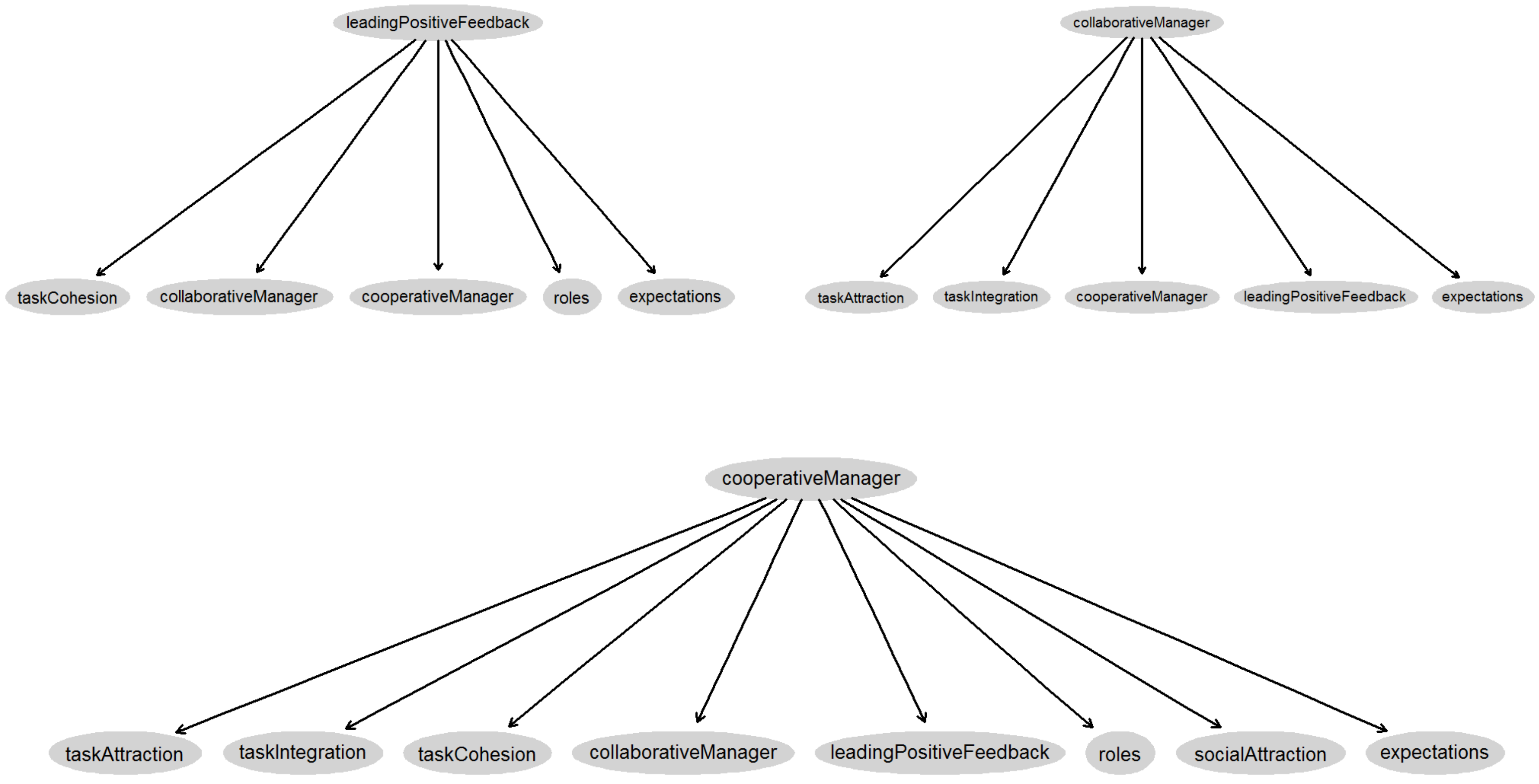
BN models estimate the joint probability distribution P over a vector of random variables X $=(X_1,\dots ,X_n)$. The joint probability distribution factorized as a product of several conditional distributions denotes the dependency/independency structure by a DAG:

$$P(X_1,\dots ,X_n)=\prod _{i=1}^{n}P(X_i\mid Pa(X_i^{\mathcal{G}})).$$

(3)

Equation (3) (where $Pa(X_i^{\mathcal{G}})$ denotes the parent nodes of $X_i$) is the main reason for the formulation of a multivariate distribution by BNs; this equation is also called the chain rule for Bayesian networks.

In order to obtain the DAG, we used the bnlearn package [43] of the R language [44]. To obtain the structure, two options either select a single best model or obtain some average model, which is known as model averaging [45]. Our model was learned by tabu algorithm, which explore the search space starting from a network structure and adding, deleting or reversing one arc at a time until the score can no longer be improved. The final model was obtained by repeating several times the structure learning; a large number of network structures was explored (1000 BNs) to reduce the impact of locally optimal (but globally suboptimal) network learning. The networks learned were averaged to obtain a more robust model. The averaged network structure was obtained using the arcs present in at least $85\%$ of the networks, which gives a measure of the strength of each arc and establishes its significance given a threshold ($85\%$) (see Figure 1 and Listing 1).

Parameters were obtained again with the bnlearn package in the R language by performing a Bayesian parameter estimation using a Dirichlet distribution [46]. A conditional probability distribution is obtained for each node.

2.3.3. Naive Bayes

The NB model assumes that instances fall into one of a number of mutually exclusive classes, and it is the simplest BN classifier, where the predictive variables are assumed to be conditionally independent given the class:

$$P({\mathbf{x}}_{\mathbf{i}}\mid c_j)=P(x_{i1}\mid c_j)\cdots P(x_{in}\mid c_j).$$

(4)

Even though the assumption of conditional independence is violated on numerous occasions in real applications, NB still performs well in many situations [41]. In Figure 2, three NB structures for leading positive feedback, cooperative manager and collaborative manager are obtained from the bnlearn package [43] in the R language [44] (see also Listing 2).

The joint probability distribution for the NB models in Figure 2 by simple probabilistic reasoning and then the conditional independence assumption for a NB model are obtained as follows.

Suppose $C=leadingPositiveFeedback$, $X_1=expectations$, $X_2=collaborativeManager$, $X_3=cooperativeManager$, $X_4=roles$, $X_5=taskCohesion$, then:

$$P(C,X_1,X_2,X_3,X_4,X_5)=P(X_1,X_2,X_3,X_4,X_5|C)·P(C)=\prod _{i=1}^{5}P(X_i|C)·P(C).$$

(5)

If we suppose $C=cooperativeManager$, $X_1=taskCohesion$, $X_2=socialAttraction$, $X_3=taskIntegration$, $X_4=collaborativeManager$, $X_5=leadingPositiveFeedback$, $X_6=roles$, $X_7=expectations$, $X_8=taskAttraction$, then we can have:

$$\begin{array}{cc}& P(C,X_1,X_2,X_3,X_4,X_5,X_6,X_7,X_8)=P(X_1,X_2,X_3,X_4,X_5,X_6,X_7,X_8|C)·P(C)=\hfill \\ & \prod _{i=1}^{8}P(X_i|C)·P(C).\hfill \end{array}$$

(6)

Finally, we can assume that $C=collaborativeManager$, $X_1=taskAttraction$, $X_2=taskIntegration$, $X_3=cooperativeManager$, $X_4=leadingPositiveFeedback$, $X_5=expectations$; we can obtain that:

$$\begin{array}{cc}& P(C,X_1,X_2,X_3,X_4,X_5)=P(X_1,X_2,X_3,X_4,X_5|C)·P(C)=\prod _{i=1}^{5}P(X_i|C)·P(C).\hfill \end{array}$$

(7)

After the above steps, we have factorized the joint distribution as a product of conditional probability distributions. In an NB model, given the parent node, the remaining nodes are independent. Given the parent node, for each pair of nodes ${\mathbf{X}}_{\mathbf{i}}$ and ${\mathbf{X}}_{\mathbf{j}}$, by applying the symmetry property, the ${\mathbf{X}}_{\mathbf{i}}$ node is independent of ${\mathbf{X}}_{\mathbf{j}}$ and reciprocally.

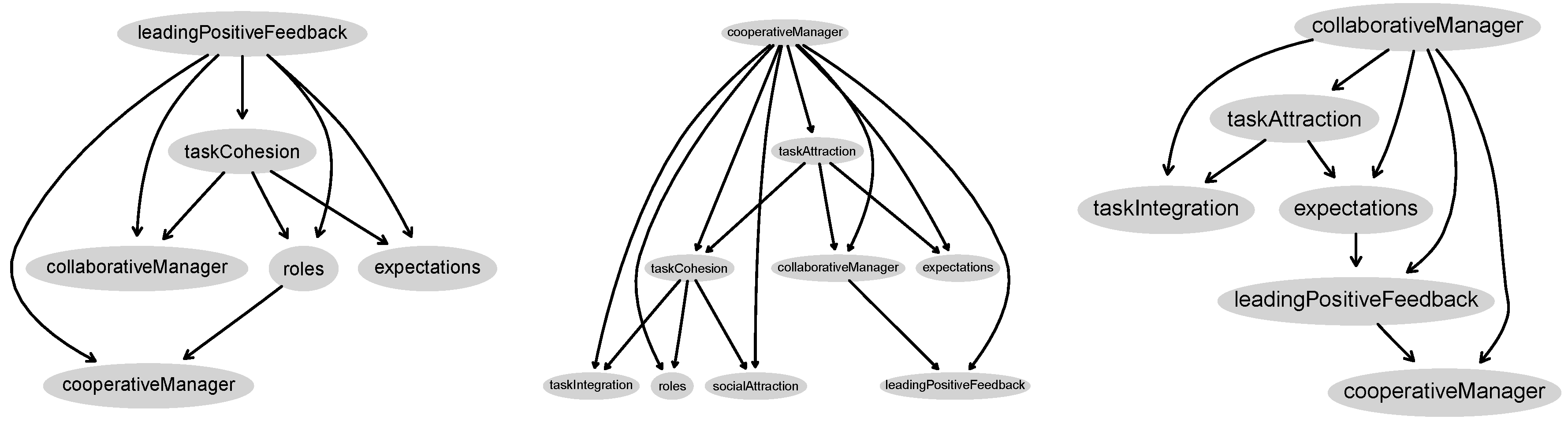
2.3.4. Tree Augmented Naive Bayes

The TAN classifier [38] extends the NB model with a tree-shaped graph across the predictor variables. The TAN model is similar to NB, except that each predictor variable is allowed to depend on other predictor variables in addition to the class. Figure 3 shows three models that we have learned for leading positive feedback, cooperative manager and collaborative manager (see also Listing 3). This model provides more information than the NB model, as it included information about the relationship among all predictor variables.

Let us note that the joint probability distribution for the TAN models in Figure 3 by simple probabilistic reasoning and then using the conditional independence assumption for a TAN model is as follows (from left to right):

We can assume that $C=leadingPositiveFeedback$, $X_1=expectations$, $X_2=collaborativeManager$, $X_3=cooperativeManager$, $X_4=roles$, $X_5=taskCohesion$:

$$P(X_1,X_2,X_3,X_4,X_5)=P(X_5|C)·P(X_2|X_5,C)·P(X_4|X_5,C)·P(X_1|X_5,C)·P(X_3|X_4,C)·P(C).$$

(8)

Now, let us suppose $C=cooperativeManager$, $X_1=taskCohesion$, $X_2=socialAttraction$, $X_3=taskIntegration$, $X_4=collaborativeManager$, $X_5=leadingPositiveFeedback$, $X_6=roles$, $X_7=expectations$, $X_8=taskAttraction$, then:

$$\begin{array}{cc}& P(C,X_1,X_2,X_3,X_4,X_5,X_6,X_7,X_8)=P(X_8|C)·P(X_1|C,X_8)·P(X_4|C,X_8)·P(X_7|C,X_8)·\hfill \\ & P(X_3|C,X_1)·P(X_6|C,X_1)·P(X_2|C,X_1)·P(X_5|C,X_4)·P(X_1).\hfill \end{array}$$

(9)

As another step, we can assume that $C=collaborativeManager$, $X_1=taskAttraction$, $X_2=taskIntegration$, $X_3=cooperativeManager$, $X_4=leadingPositiveFeedback$, $X_5=expectations$; then, we will obtain:

$$\begin{array}{cc}& P(C,X_1,X_2,X_3,X_4,X_5)=P(X_1|C)·P(X_2|X_1,C)·P(X_5|X_1,C)·P(X_4|X_5,C)·\hfill \\ & P(X_3|X_4,C)·P(C).\hfill \end{array}$$

(10)

Up to this point, we obtain the probabilistic models factorized according to the TAN models, which are special types of BNs; see Figure 3. The independence of the social attraction and leading positive feedback features given the roles and cooperative manager features is shown in the center of Figure 3; reciprocally by symmetry, leading positive feedback is independent of the social attraction given the roles and cooperative manager features. Similarly, on the right side of Figure 3, cooperative manager and task integration appear as independent features given the collaborative manager and task cohesion features.

2.3.5. Validation

The models are validated using a 10-fold cross-validation. In

Table 1. AUCs and the percentage correctly classified for the different features by the Bayesian network (BN).

Variable Name	AUC	Accuracy
Task Attraction	0.8834 (±0.0038)	87.3450% (±0.2280)
Task Integration	0.8898 (±0.0034)	90.5707% (±0.4290)
Task Cohesion	0.9747 (±0.0033)	93.3002% (±0.3833)
Collaborative Manager	0.8011 (±0.0023)	87.0968% (±0.3133)
Cooperative Manager	0.7745 (±0.0041)	84.6154% (±0.3255)
Leading Positive Feedback	0.7851 (±0.0026)	90.0744% (±0.3265)
Experience	0.6250 (±0.0110)	80.6951% (±0.3519)
Roles	0.7450 (±0.0037)	95.7816% (±0.3050)
Social Attraction	0.6772 (±0.0103)	78.4119% (±0.3400)
Expectations	0.7100 (±0.0030)	76.4268% (±0.3781)

Standard deviation between brackets.

, the area under the ROC curve (AUC) and the percentage correctly classified for the different features in the BN model are shown.

2.3.6. Performance Comparison

In order to provide reference benchmarks about how our BN classifies the features, we compare it to other classification performances. The performance of each classification model is evaluated using four statistical measures: accuracy, sensitivity, specificity and precision. Classification accuracy is defined as the ratio of the number of correctly-classified cases. The sensitivity refers to the rate of correctly classified as positive. The specificity refers to the rate of correctly classified as negative, and the precision refers to the rate of positive predicted value. Other classifiers have also been considered to compare to the Bayesian classifiers: the multilayer perceptron (MP) [48], logistic regression (LR) [49], Id3 [50] and random forest (RF) [51] algorithms. The best performance is obtained by the average BN and TAN models (see

Table 2. Comparison of the accuracy and other metrics for the leading positive feedback feature using different algorithms. MP, multilayer perceptron.

Algorithms	Accuracy	Sensitivity	Specificity	Precision
BN	90.07% (±0.3265)	0.9178 (±0.0024)	0.6538 (±0.0039)	0.9746 (±0.0032)
NB	88.09% (±0.3519)	0.8810 (±0.0035)	0.6470 (±0.0005)	0.8590 (±0.0033)
TAN	90.07% (±0.3342)	0.9156 (±0.0030)	0.6667 (±0.0053)	0.9775 (±0.0048)
MP	88.83% (±0.3267)	0.8880 (±0.0033)	0.6640 (±0.0232)	0.8660 (±0.0059)
LR	88.09% (±0.3781)	0.8810 (±0.0038)	0.7550 (±0.0269)	0.8480 (±0.0082)
Id3	88.09% (±0.3708)	0.8810 (±0.0038)	0.7550 (±0.0247)	0.8480 (±0.0132)
RF	88.09% (±0.3400)	0.8810 (±0.0034)	0.7550 (±0.0356)	0.8480 (±0.0073)

Standard deviation between brackets.

,

Table 3. Comparison of the accuracy and other metrics for the cooperative manager feature using different algorithms.

Algorithms	Accuracy	Sensitivity	Specificity	Precision
BN	82.63% (±0.3255)	0.8329 (±0.0036)	0.7500 (±0.0062)	0.9748 (±0.0058)
NB	75.68% (±0.4598)	0.7570 (±0.0047)	0.5400 (±0.0054)	0.7420 (±0.0041)
TAN	83.87% (±0.3638)	0.8462 (±0.0043)	0.7692 (±0.0028)	0.9716 (±0.0022)
MP	76.67% (±1.1174)	0.7670 (±0.0110)	0.5460 (±0.0194)	0.7470 (±0.0103)
LR	79.40% (±0.6455)	0.7940 (±0.0064)	0.5730 (±0.0114)	0.7650 (±0.0088)
Id3	80.89% (±0.6129)	0.8090 (±0.0061)	0.5690 (±0.0171)	0.7840 (±0.0094)
RF	80.40% (±1.1219)	0.8040 (±0.0113)	0.5280 (±0.0203)	0.7820 (±0.0138)

Standard deviation between brackets.

and

Table 4. Comparison of the accuracy and other metrics for the collaborative manager feature using different algorithms.

Algorithms	Accuracy	Sensitivity	Specificity	Precision
BN	87.10% (±0.3642)	0.9829 (±0.0068)	0.5000 (±0.0108)	0.9829 (±0.0062)
NB	84.86% (±0.2280)	0.8490 (±0.0023)	0.7100 (±0.0139)	0.8180 (±0.0036)
TAN	87.09% (±0.3826)	0.8824 (±0.0036)	0.5000 (±0.0042)	0.9829 (±0.0096)
MP	86.85% (±0.4290)	0.8680 (±0.0041)	0.8060 (±0.0233)	0.8220 (±0.0101)
LR	86.85% (±0.3813)	0.8680 (±0.0033)	0.8220 (±0.0007)	0.8180 (±0.0081)
Id3	86.85% (±0.3139)	0.8680 (±0.0030)	0.8390 (±0.0119)	0.8130(±0.0118)
RF	86.35% (±0.5290)	0.8640 (±0.0053)	0.7570 (±0.0247)	0.8230 (±0.0094)

Standard deviation between brackets.

). However, some of these models also show a low specificity for the collaborative manager model and leading positive feedback by increasing the Type I error (one-specificity).

Furthermore, BNs are able to produce probability estimates. In this sense, we are interested in knowing the features with the highest influence in maximizing collective efficacy, cooperative manager and collaborative manager in the high and low states.

2.3.7. Conditional Entropy

In Shannon [47] theory, the entropy of X is the lower bound on the average number of bits that are needed to encode values of X. Another way of viewing the entropy is as a measure of our uncertainty about the value of X, i.e., lower uncertainty about X will produce a low entropy value.

A natural question is what is the cost of encoding X if we have already encoded Y. The conditional entropy of X given Y is:

$$H_P(X|Y)=E_P[log\frac{1}{P(X|Y)}]=\sum P(X|Y)·log\frac{1}{P(X|Y)}$$

(11)

which captures the additional cost (in terms of bits) of encoding X when we have already encoded $Y.$ Note that the maximum value of probability in $P(X|Y)$ implies the lowest entropy value.

For the leading positive feedback, cooperative manager and collaborative manager features, we are interested in determining and ordering the state values for conditioned features, because we can obtain the maximum probability value in the low state and the high state. This will lead to achieving the desired minimum conditioned entropy.

3. Results

The BN model has been selected to rank the features that can mostly increase the probability value of leading positive feedback, or cooperative manager, or collaborative manager in a specific state value.

Given the evidence E = e, our goal is to find the most likely assignment to the remaining variables, denoted by $\mathbf{U}$; see Equation (12):

$$MAP(\mathbf{U}\mid e)=argma{x}_{u}P(u,e)$$

(12)

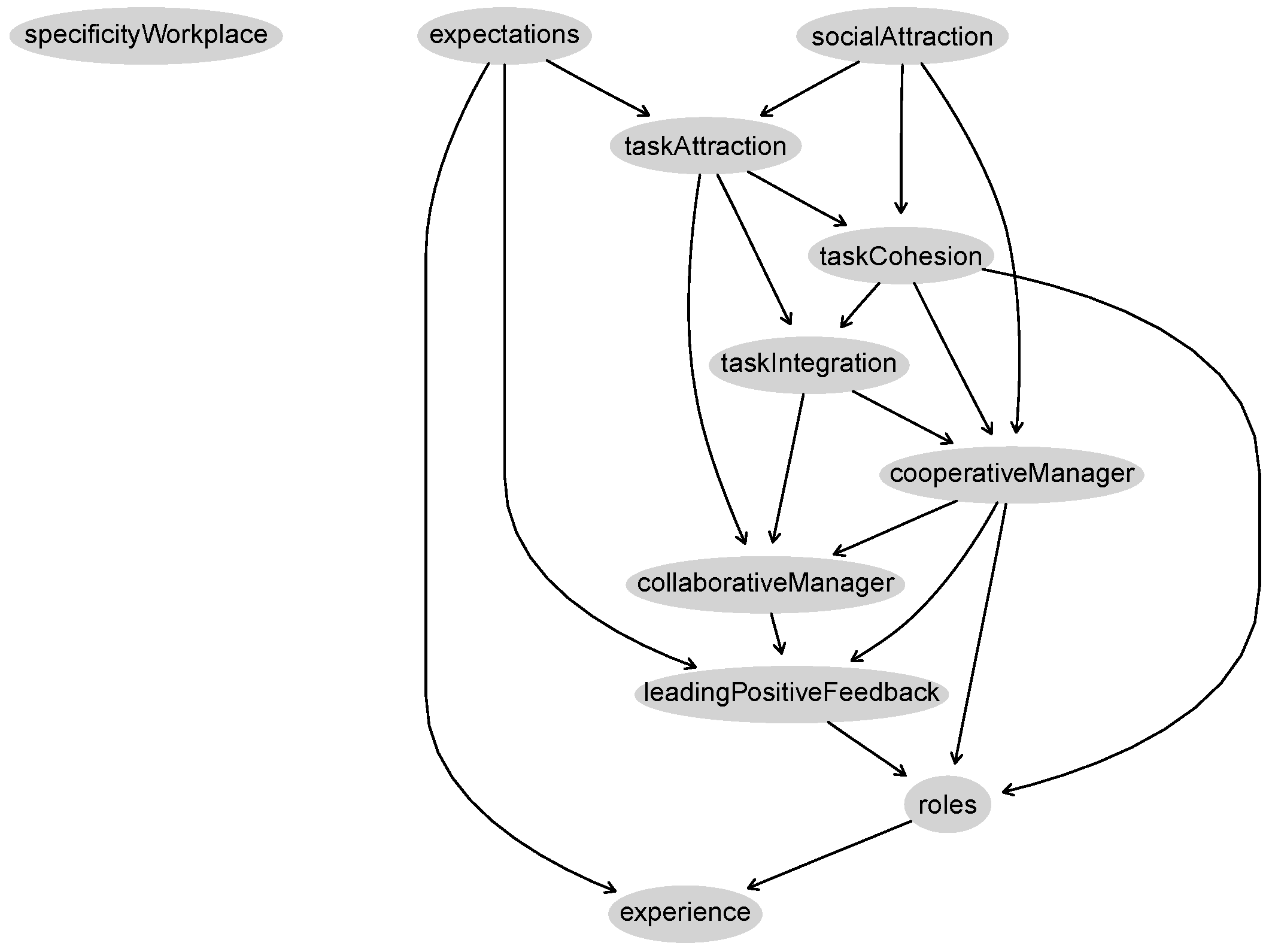
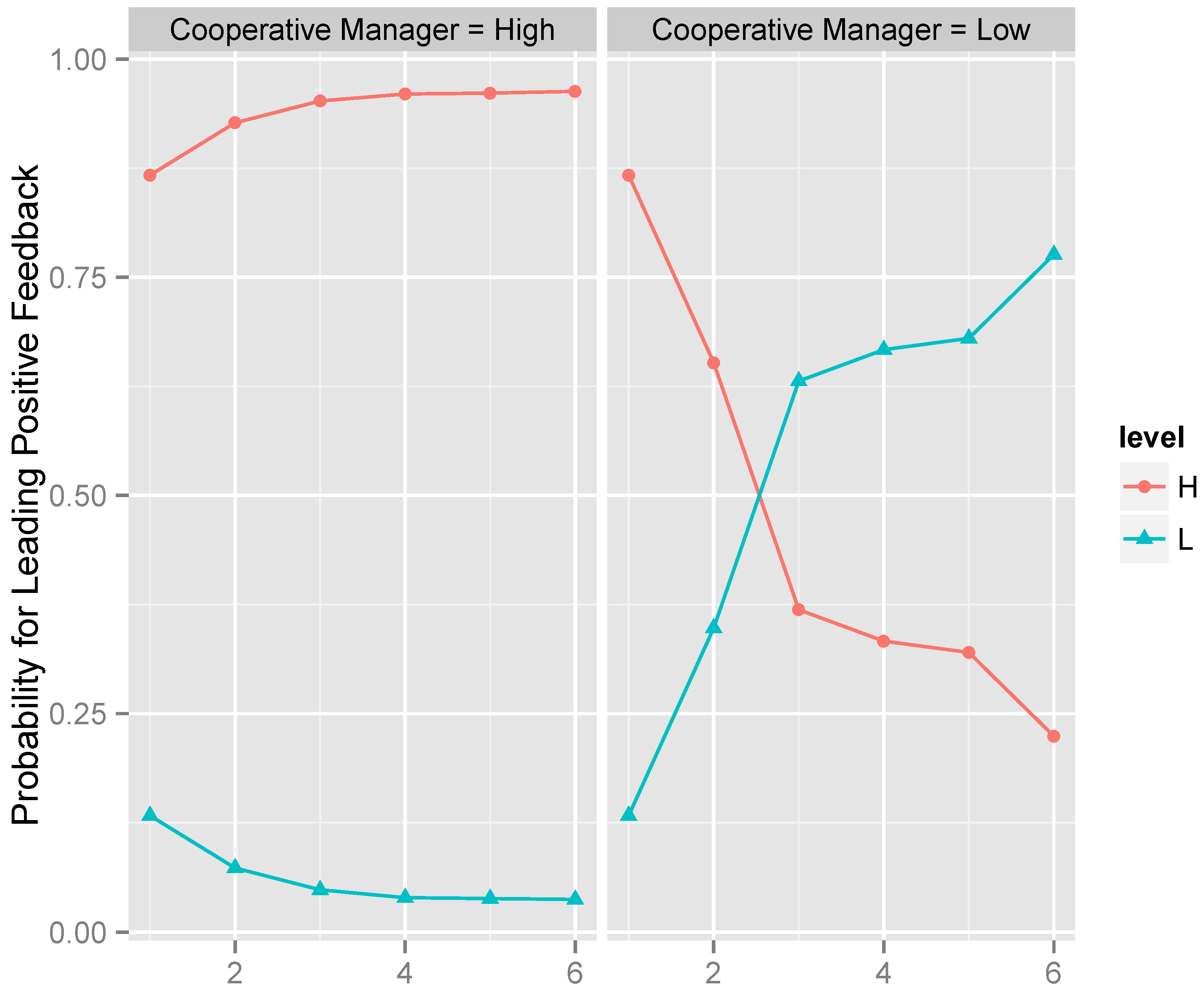
3.1. BN Model for Leading Positive Feedback

We select at each step the feature that maximize the most leading positive feedback feature likelihood in a high state, i.e., we choose from each step the variable and the state that induces the greatest increase in the likelihood of leading positive feedback variable in a high state. A summary is shown in

Table 5. Step-by-step instantiations leading to maximization of the likelihood of the leading positive feedback variable in its high state.

Step	Instantiated Variable		Value	Leading Positive Feedback = High
1	none	=	–	$86.7\%$
2	cooperative manager	=	High	$92.7\%$
3	expectations	=	Low	$95.2\%$
4	collaborative manager	=	High	$96.0\%$
5	roles	=	High	$96.1\%$
6	task cohesion	=	Low	$96.3\%$

and Figure 4 (on the right side).

As shown in Table 5, we can use a step by step instantiation method to maximize the likelihood of the “leading positive feedback” feature. At Step 1, with no values set for other features in the initial BN, we can reach a likelihood of $86.7\%$. At the subsequent steps, we add the conditions for the instantiation of other features one by one as indicated in Table 5; in each step, the percentage of the likelihood of the “leading positive feedback” increases accordingly and finally reached $96.3\%$.

Table 6. Step-by-step instantiations leading to the maximization of the likelihood of the leading positive feedback variable in its low state.

Step	Instantiated Variable		Value	Leading Positive Feedback = Low
1	none	=	–	$13.3\%$
2	cooperative manager	=	Low	$34.8\%$
3	collaborative manager	=	Low	$63.1\%$
4	expectations	=	High	$66.7\%$
5	roles	=	High	$68.0\%$
6	task cohesion	=	Low	$77.6\%$

,

Table 7. Step-by-step instantiations leading to the maximization of the likelihood of the cooperative manager variable in its high state.

Step	Instantiated Variable		Value	Cooperative Manager = High
1	none	=	–	$78.1\%$
2	leading positive feedback	=	High	$83.6\%$
3	task cohesion	=	High	$86.0\%$
4	social attraction	=	High	$87.4\%$
5	expectations	=	High	$87.8\%$
6	collaborative manager	=	High	$88.5\%$
7	task attraction	=	High	$89.0\%$
8	task integration	=	High	$89.2\%$
9	roles	=	High	$89.3\%$

,

Table 8. Step-by-step instantiations leading to the maximization of the likelihood of the cooperative manager variable in its low state.

Step	Instantiated Variable		Value	Cooperative Manager = Low
1	none	=	–	$21.9\%$
2	leading positive feedback	=	Low	$57.2\%$
3	collaborative manager	=	Low	$73.7\%$
4	roles	=	Low	$82.6\%$
5	task attraction	=	High	$90.1\%$
6	task integration	=	High	$93.5\%$
7	social attraction	=	Low	$96.1\%$
8	expectations	=	Low	$96.4\%$
9	task cohesion	=	High	$96.5\%$

,

Table 9. Step-by-step instantiations leading to the maximization of the likelihood of the collaborative manager variable in its high state.

Step	Instantiated Variable		Value	Collaborative Manager = High
1	none	=	–	$85.5\%$
2	task attraction	=	High	$90.7\%$
3	cooperative manager	=	High	$93.3\%$
4	task integration	=	High	$95.4\%$
5	leading positive feedback	=	High	$95.7\%$
6	expectations	=	Low	$95.8\%$

and

Table 10. Step-by-step instantiations leading to the maximization of the likelihood of the collaborative variable in its low state.

Step	Instantiated Variable		Value	Collaborative Manager = Low
1	none	=	–	$14.5\%$
2	leading positive feedback	=	Low	$34.9\%$
3	task integration	=	Low	$58.0\%$
4	task attraction	=	Low	$66.1\%$
5	expectations	=	Low	$76.3\%$
6	cooperative manager	=	Low	$81.4\%$

list the same step by step method to maximize the likelihood of other features.

Again, we choose from each step the variable and the state that induces the greatest increase in the likelihood of the leading positive feedback variable in a low state. A summary is shown in Table 6 and Figure 4 (on the left side).

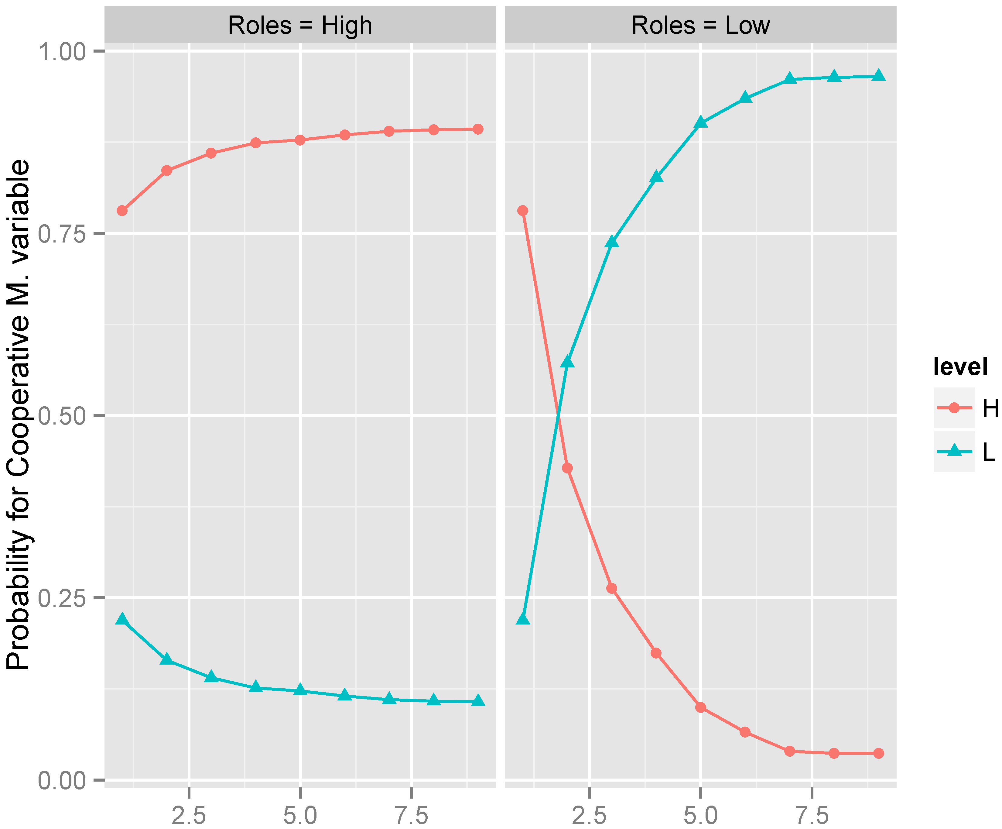
3.2. BN Model for the Cooperative Manager

We select at each step the feature that maximize the greatest cooperative manager feature likelihood in a high state, i.e., we choose from each step the variable and the state that induce the greatest increase in the likelihood of the cooperative manager variable in a high state. A summary is shown in Table 7 and Figure 5.

Again, we choose from each step the variable and the state that induces the greatest increase in the likelihood of the cooperative manager variable in a low state. In this case, the cooperative manager achieves the maximum in the low state when leading positive feedback and roles are instantiated in a low value; however, to see the influence of the other features, we show the roles feature in the last position. A summary is shown in Table 8 and Figure 5 (on the right side).

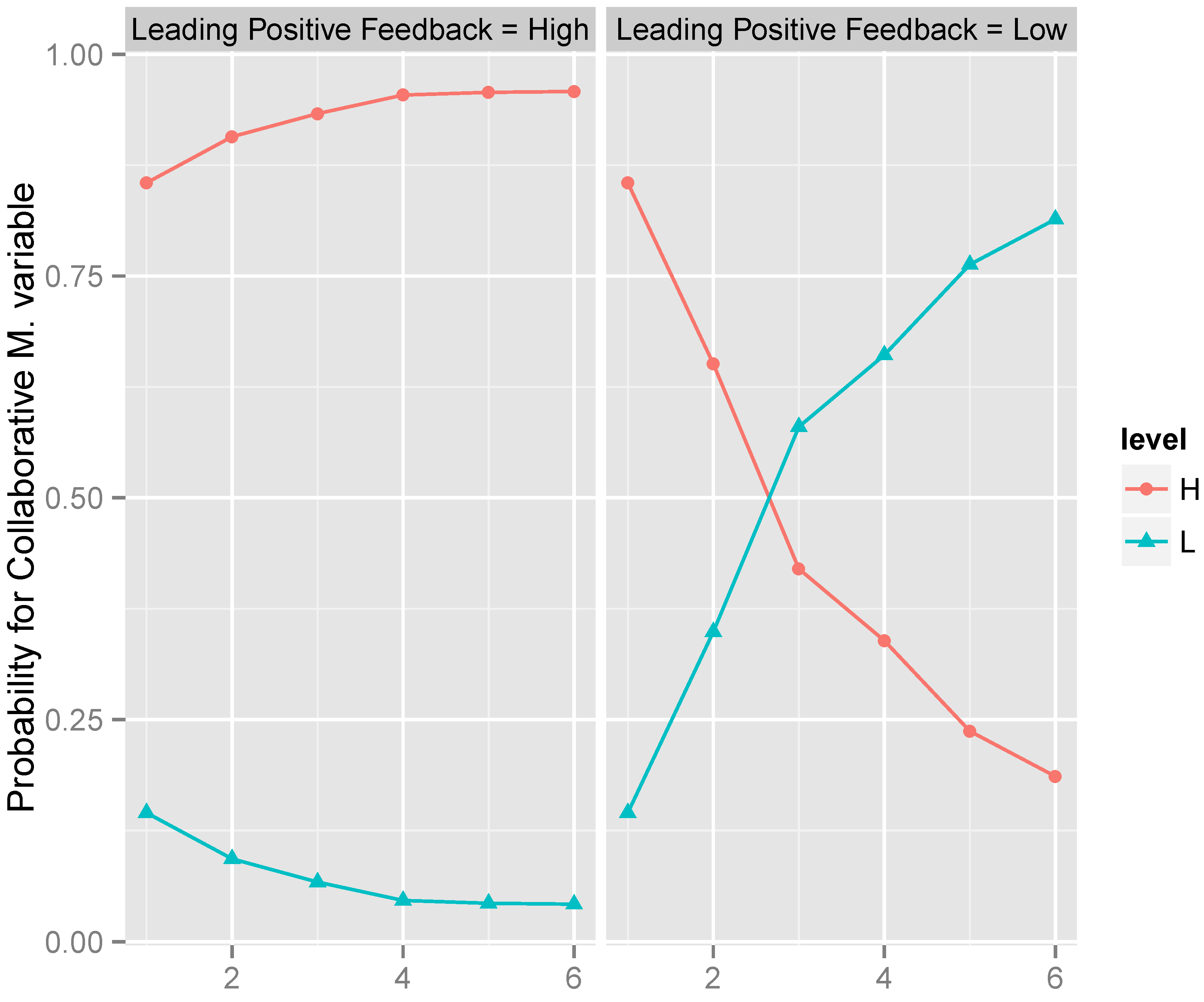
3.3. BN Model for the Collaborative Manager

We select at each step the feature that maximize the greatest collaborative manager feature likelihood in a high state, i.e., we choose from each step the variable and the state that induce the greatest increase in the likelihood of the collaborative manager variable in a high state. A summary is shown in Table 9 and Figure 6 (on the right side).

Again, we choose from each step the variable and the state that induce the greatest increase in the likelihood of the collaborative manager variable in a low state. In this case, the cooperative manager achieves the maximum in the low state when the features task attraction, leading positive feedback, task cohesion, experience, cooperative manager and task integration are all instantiated in a low state. A summary is shown in Table 10 and Figure 6 (on the left side).

4. Discussion

In this study, ranking the psychological team features is pretty relevant attending to the manager’s and coaches’ great difficulties in generating specific climates addressed to obtain better performance from the team members acting as a whole team [53,55].

At present, there is still discussion about the extrapolation of the mechanisms of the teams and their tasks; however, there is a common agreement on the importance of the concept of cohesion, leadership and the specific working position [9,10,54,55,56]. From this point of view, this set of concepts has been considered as a prototype for racing sports teams and should be discussed in terms of the relationship with the group performance. In previous works [52], the relationships between some features were established. In this study, we used the Markov blanket in the average BN to determine a different subset of features. After, two BN classifiers are determined. The aim of this study has been reached through the elaboration of the BN, the subsequent TANs and some major instantiations. Our study shows the importance of the role played by social attraction (as was predicted by Carron and Eys ([2,9,36]) and the team members’ expectations, as was outlined when studying the role of self-efficacy related to the teams’ performance [8]. These two variables appear as the BN antecessors, influencing the rest of the variables. Furthermore, in our study, the main node has been found to be the cooperative teamwork style (as has been outlined in previous studies [13,20,52]); it determines the BN bottom consequences, the members roles and their experience, i.e., their time duration for playing on the same team. These two consequences are critical for the determination of the team performance and their stability across different situations. However, there may be a distortion of objectivity due to the team affective attraction, which can possibly affect the members’ trust of the team’s capabilities [53]. When we conduct instantiations on the BN and maximize leading positive feedback managerial behavior in high and low states, BN showed the cooperative manager as the one with the strongest influence. A very interesting finding was that the initial expectations about the team performance need to be low in case the leading positive feedback is maximized to high, and it needs to be high in case the leading positive feedback is maximized to low, in agreement with previous work [20]. After that, knowing under which features the cooperative manager would work with maximum probability in high and low states is quite important. When we instantiated the cooperative manager feature in the maximum of high and low states, BN showed, not surprisingly, leading positive feedback as the one with the strongest influence. Adding roles in high and low states, we maximize the cooperative manager in high and low states, respectively, achieving an entropy with a value of zero. The other variables that have shown influence on the cooperative managerial style are the social attraction, the specificity of the workplace and the roles when the style is maximized to both low and high states. Maximizing the collaborative manager feature in high and low states is also of special interest, showing its contribution to the main cooperative node. It appears that when we maximize the collaborative manager in a high state, the task attraction is the variable with the strongest influence, followed by the cooperative manager, task integration (instantiated in the high state), leading positive feedback and, finally, expectations (when team members behave as being focused just on reaching the team’s objectives). On the other hand, the task integration can be instantiated in a low state in case we are interested in maximizing the collaborative manager to the low state.

5. Conclusions

In the study of sports science and other cooperative work systems, BNs provide some major advantages. They explicitly provide the conditional probability distributions of the values of every feature given the values of other input features. They are represented in a clear, appealing way, and are very easy to comprehend and translate to end users, i.e., managers and coaches. In this study, by the ranking obtained from the BN among the psychological variables, we come to the conclusion that the cooperative style with its associated behaviors constitutes the most prominent psychological variable. Managers have to work with team members’ expectations and the social aspects of the job, because they are the antecessors of the whole BN, and also, they need to keep in mind that the cooperation, developed mainly through a positive feedback work climate and a pro-social, i.e., collaborative, managerial style, leads to the correct decision of the proper assignation of team roles and the working duration of the team members.

References

1. Callow, N.; Smith, M.J.; Hardy, L.; Arthur, C.A.; Hardy, J. Measurement of transformational leadership and its relationship with team cohesion and performance level. J. Appl. Sport Psychol. 2009, 22, 395–412. [Google Scholar] [CrossRef]
2. Carron, A.V.; Brawley, L.R.; Widmeyer, W.N. Measurement of cohesion in sport and exercise. In Advances in Sport and Exercise Psychology Measurement; Duda, J.L., Ed.; Fitness Information Technology: Morgantown, WV, USA, 1998; pp. 213–226. [Google Scholar]
3. Heuzé, J.P.; Raimbault, N.; Fontayne, P. Relationships between cohesion, collective efficacy and performance in professional basketball teams: An examination of mediating effects. J. Sports Sci. 2006, 24, 59–68. [Google Scholar] [CrossRef] [PubMed]
4. Myers, N.D.; Payment, C.A.; Feltz, D.L. Reciprocal relationships between collective efficacy and team performance in women’s ice hockey. Group Dyn.-Theor. Res. 2004, 8, 182–195. [Google Scholar] [CrossRef]
5. Wilson, D.S.; Ostrom, E.; Cox, M.E. Generalizing the core design principles for the efficacy of groups. J. Econ. Behav. Organ. 2013, 90S, S21–S32. [Google Scholar] [CrossRef]
6. Mathieu, J.; Maynard, M.T.; Rapp, T.; Gilson, L. Team effectiveness 1997-2007: A review of recent advancements and a glimpse into the future. J. Manag. 2008, 34, 410–476. [Google Scholar] [CrossRef]
7. Cannon-Bowers, J.A.; Salas, E. Teamwork competencies: The interaction of team members knowledge, skills, and attittudes. In Workforce Readiness: Competencies and Assessment; O’Neil, H.F., Ed.; Erlbaum: Mahwah, NJ, USA, 1997; pp. 151–174. [Google Scholar]
8. Fuster-Parra, P.; García-Mas, A.; Ponseti, F.J.; Leo, F.M. Team performance and collective efficacy in the dynamic psychology of competitive team: A Bayesian network analysis. Hum. Mov. Sci. 2015, 40, 98–118. [Google Scholar] [CrossRef] [PubMed]
9. Beal, D.J.; Cohen, R.R.; Burke, M.J.; McLendon, C.L. Cohesion and performance in groups: A meta-analytic clarification of construct relations. J. Appl. Psychol. 2003, 88, 989–1004. [Google Scholar] [CrossRef] [PubMed]
10. Carron, A.V.; Bray, S.R.; Eys, M.A. Team cohesion and team success in sport. J. Sports Sci. 2002, 20, 119–126. [Google Scholar] [CrossRef] [PubMed]
11. Eys, M.A.; Carron, A.V.; Beauchamp, M.R.; Bray, S.R. Role ambiguity in sport teams. J. Sport Exerc. Psychol. 2003, 25, 534–550. [Google Scholar]
12. Jirotka, M.; Gilbert, N.; Luff, P. On the social organisation of organisations. Comput. Support. Coop. Work J. 1992, 1, 95–118. [Google Scholar] [CrossRef]
13. Lameiras, J.; Almeida, P.L.; García-Mas, A. Relationships between cooperation and goal orientation among male professional and semi-professional team athletes. Percept. Motor Skills 2014, 119, 851–860. [Google Scholar] [CrossRef] [PubMed]
14. Heckerman, D. Bayesian networks for data mining. Data Min. Knowl. Discov. 1997, 1, 79–119. [Google Scholar] [CrossRef]
15. Jensen, F.V.; Nielsen, T.D. Bayesian Networks and Decision Graphs; Information Science & Statistics; Springer: Berlin/Heidelberg, Germany; New York, NY, USA, 2007. [Google Scholar]
16. Koller, D.; Friedman, N. Probabilistic Graphical Models. Principles and Techniques; The MIT Press: Cambridge, MA, USA; London, UK, 2010. [Google Scholar]
17. Korb, K.B.; Nicholson, A.E. Bayesian Artificial Intelligence; Chapman and Hall/CRC Press: London, UK, 2010. [Google Scholar]
18. Pearl, J. Causality. Models, Reasoning and Inference; Cambridge University Press: Cambridge, UK, 2000. [Google Scholar]
19. Fuster-Parra, P.; García-Mas, A.; Ponseti, F.J.; Palou, P.; Cruz, J. A Bayesian network to discover relationships between negative features in sport: A case study of teen players. Qual. Quant. 2014, 48, 1473–1491. [Google Scholar] [CrossRef]
20. Fuster-Parra, P.; García-Mas, A.; Cantallops, J.; Ponseti, F.J. Cooperative team work analysis and modeling: A Bayesian network approach. In Cooperative Design, Visualization and Engineering; Luo, Y., Ed.; Springer International Publishing: Berlin, Germany, 2015; pp. 1–10. [Google Scholar] [CrossRef]
21. Fuster-Parra, P.; Tauler, T.; Bennasar-Veny, M.; Ligȩza, A.; López-González, A.A.; Aguiló, A. Bayesian network modeling: A case study of an epidemiologic system analysis of cardiovascular risk. Comput. Methods Progr. Biomed. 2016, 126, 128–142. [Google Scholar] [CrossRef] [PubMed]
22. DeFelipe, J.; López-Cruz, P.L.; Benavides-Piccione, R.; Bielza, C.; Larrañaga, P.; Anderson, S.; Burkhalter, A.; Cauli, B.; Fairén, A.; Feldmeyer, D.; et al. New insights into the classification and nomenclature of cortical GABAergic interneurons. Nat. Neurosci. 2013, 14, 202–216. [Google Scholar] [CrossRef] [PubMed] [Green Version]
23. Ligȩza, A.; Fuster-Parra, P. AND/OR/NOT causal graphs. A model for diagnostic reasoning. Int. J. Appl. Math. Comput. Sci. 1997, 7, 185–203. [Google Scholar]
24. Cooper, G.F.; Herskovits, E. A Bayesian method for the induction of probabilistic networks from data. Mach. Learn. 1992, 9, 309–347. [Google Scholar] [CrossRef]
25. Heckerman, D.; Geiger, D.; Chickering, D.M. Learning Bayesian networks: The combination of knowledge and statistical data. Mach. Learn. 1995, 20, 197–243. [Google Scholar] [CrossRef]
26. Butz, C.J.; Hua, S.; Chen, J.; Yao, H. A simple graphical approach for understanding probabilistic inference in Bayesian networks. Inf. Sci. 2009, 179, 699–716. [Google Scholar] [CrossRef]
27. Glymour, C. The Mind’s Arrows: Bayes Nets and Graphical Causal Models in Psychology; The MIT Press: New York, NY, USA, 2003. [Google Scholar]
28. Druzdzel, M.J.; Glymour, C. What do college ranking data tell us about student retention: Causal discovery in action. Intelligent Information Systems IV. In Proceedings of the Workshop Held in Augustów, Poland, 5–9 June 1985; pp. 1–10.
29. Glymour, C.; Scheines, R.; Spirtes, P.; Kelly, K. Discovering Causal Structure; Academic Press: New York, NY, USA, 1987. [Google Scholar]
30. Spirtes, P.; Glymour, C.; Scheines, R. Causation, Prediction and Search, 2nd ed.; Adaptive Computation and Machine Learning; The MIT Press: New York, NY, USA, 2001. [Google Scholar]
31. Darwiche, A. Bayesian networks. In Handbook of Knowledge Representation, Foundations of Artificial Intelligence; Van Harmelen, A., Lifschitz, V., Porter, B., Eds.; Elsevier: Amsterdam, The Netherlands, 2008; p. 1034. [Google Scholar]
32. Witten, I.H.; Frank, E. Data Mining: Practical Machine Learning Tools and Techniques; Morgan Kaufman: Amsterdam, The Netherlands, 2005. [Google Scholar]
33. Felipe, S.C.; Pires, D.S.; Nassar, S.M. Analysis of bayesian classifier accuracy. J. Comput. Sci. 2013, 9, 1487–1495. [Google Scholar]
34. García Mas, A.; Fuster-Parra, P.; Ponseti, J.; Palou, P.; Olmedilla, A.; Cruz, J. Análisis de las relaciones entre motivación, el clima motivacional y la ansiedad competitiva entre jóvenes jugadores de equipo mediante una red Bayesiana. An. Psicol.-Spain 2015, 1, 355–366. [Google Scholar] [CrossRef]
35. Crespo, M.; Balaguer, I.; Atienza, F.L. Análisis psicométrico de la versión española de la escala de liderazgo en el deporte de Chelladurai y Saleh en la versión de entrenadores. Rev. Psicol. Soc. AP 1994, 4, 5–28. [Google Scholar]
36. Carron, A.V.; Eys, M.A. Group Dynamics in Sport; Fitness Information Technology: Morgantown, WV, USA, 2012. [Google Scholar]
37. Iturbide, L.M.; Elosua, P.; Yanes, F. Medida de la cohesión en equipos deportivos. Adaptación al español del Group Environment Questionnaire (GEQ). Psicothema 2010, 22, 482–488. [Google Scholar] [PubMed]
38. Friedman, N.; Geiger, D.; Goldszmidt, M. Bayesian network classifiers. Mach. Learn. 1997, 29, 131–163. [Google Scholar] [CrossRef]
39. Duda, R.; Hart, P.; Stork, D. Pattern Classification; John Wiley and Sons: New York, NY, USA, 2001. [Google Scholar]
40. Bielza, C.; Larrañaga, P. Discrete Bayesian network classifiers: A survey. ACM Comput. Surv. 2014, 47, 5:1–5:43. [Google Scholar] [CrossRef]
41. Domingos, P.; Pazzani, M. On the optimality of the simple Bayesian classifier under zero-one loss. Mach. Learn. 1997, 29, 103–130. [Google Scholar] [CrossRef]
42. Nagarajan, R.; Scutari, M.; Lèbre, S. Bayesian Networks in R: With Applications in Systems Biology; Springer: Berlin/Heidelberg, Germany; New York, NY, USA, 2013. [Google Scholar]
43. Scurati, M. Learning Bayesian networks with the bnlearn R package. J. Stat. Softw. 2010, 35, 1–22. [Google Scholar]
44. R Development Core Team. R: A Language and Environment for Statistical Computing; [Computer Software]; R Foundation for Statistical Computing: Vienna, Austria; Available online: http://www.R-project.org/ (accessed on 20 March 2012).
45. Claeskens, G.; Hjort, N.L. Model Selection and Model Averaging; Cambridge University Press: Cambridge, UK, 2008. [Google Scholar]
46. Neapolitan, N.E. Learning Bayesian Networks; Prentice Hall, Inc.: Upper Saddle River, NJ, USA, 2003. [Google Scholar]
47. Shannon, C.E. A mathematical theory of communication. Bell. Labs Tech. J. 1948, 27, 379–423. [Google Scholar] [CrossRef]
48. Haykin, S. Neural Networks: A Comprenhensive Foundation; Prentice Hall: New York, NY, USA, 1989. [Google Scholar]
49. Hosmer, D.W.; Lemeshow, S. Applied Logistic Regression; John Wiley & Sons, Inc.: Hoboken, NJ, USA, 2000. [Google Scholar]
50. Quinlan, J.R. Induction of decision trees. Mach. Learn. 1986, 1, 81–106. [Google Scholar] [CrossRef]
51. Breiman, L. Random forests. Mach. Learn. 2001, 45, 5–32. [Google Scholar] [CrossRef]
52. Olmedilla, A.; Ortega, E.; Almeida, P.; Lameiras, J.; Villalonga, T.; Sousa, C.; Torregrosa, M.; Cruz, J.; Garcia-Mas, A. Cohesión y cooperación en equipos deportivos. An. Psicol. 2011, 27, 232–238. [Google Scholar]
53. Costa, A. Work team Trust and efectiveness. Pers. Rev. 1994, 32, 605–672. [Google Scholar] [CrossRef]
54. Cohen, S.G.; Bailey, D.E. What makes team work: Group effectiveness research from the shop floor to the executive suite. J. Manag. 1997, 23, 239–290. [Google Scholar] [CrossRef]
55. Rico, R.; Alcover de la Hera, C.M.; Tabernero, C. Efectividad de los equipos de trabajo: Una revisión de la última década de investigación (1999–2009) (Efectiveness of Workteams: A review over the last decade of research (1999–2000). Rev. Psicol. Trab. Organ. 2010, 26, 47–71. [Google Scholar]
56. Taggar, S.; Brown, T.C. Problem-solving team behaviors: Development and validation of BOS and a hierarchical factor structure. Small Group Res. 2001, 32, 698–726. [Google Scholar] [CrossRef]
Figure 1. Structure obtained by model averaging over 1000 networks. It was built with the tabu learning algorithm from the bnlearn package in the R language using a threshold = 0 . 85 .
Symmetry 08 00034 g001
Figure 2. NB structures obtained using the bnlearn package in the R language for leading positive feedback, cooperative manager and collaborative manager.
Symmetry 08 00034 g002
Figure 3. Three tree augmented naive Bayes (TAN) structures obtained using the bnlearn package in the R language for leading positive feedback, cooperative manager and collaborative manager.
Symmetry 08 00034 g003
Figure 4. Step by step instantiations in the BN to maximize the leading positive feedback feature values in high and low states. The horizontal line represents the different steps from Table 6 and Table 7.
Symmetry 08 00034 g004
Figure 5. Step by step instantiations in the BN to maximize the cooperative manager feature in high and low states. The horizontal line represents the different steps from Table 8 and Table 9.
Symmetry 08 00034 g005
Figure 6. Step by step instantiations in the BN to maximize the collaborative manager feature in high and low states. The horizontal line represents the different steps from Table 8 and Table 9.
Symmetry 08 00034 g006