Article

Fluctuating Asymmetry in Two Common Freshwater Fishes as a Biological Indicator of Urbanization and Environmental Stress within the Middle Chattahoochee Watershed

by
William I. Lutterschmidt
1,*,
Samantha L. Martin
1 and
Jacob F. Schaefer
2
1
Department of Biological Sciences and the Texas Research Institute for Environmental Studies, Sam Houston State University, Huntsville, TX 77341, USA
2
Department of Biological Sciences, University of Southern Mississippi, Hattiesburg, MS 39406, USA
*
Author to whom correspondence should be addressed.
Symmetry 2016, 8(11), 124; https://doi.org/10.3390/sym8110124
Submission received: 1 September 2016 / Revised: 26 October 2016 / Accepted: 28 October 2016 / Published: 10 November 2016
(This article belongs to the Special Issue Fluctuating Asymmetry 2016)

Abstract

:
Deviations in bilateral symmetry or fluctuating asymmetry of an organism may result under environmental stressors that reduce developmental homeostasis and stability. Anthropogenic stressors such as increased urbanization can negatively impact environmental quality of aquatic ecosystems. Researchers have stressed the value in finding easy, accurate and inexpensive methods for assessing potential stress within ecosystems. Here we use fluctuating asymmetry (FA) as a useful quantitative tool in assessing the environmental quality and potential urban-based stressors within eight creeks of the Bull and Upatoi Creeks Watershed within the larger watershed of the Middle Chattahoochee. Using Geographic Information System (GIS), we characterize land-use patterns and a decreasing urbanization gradient as related to each creek’s eastward position from Columbus, Georgia. We collected two common fishes (redbreast sunfish; Lepomis auritus and bluegill; Lepomis macrochirus), measured both metric and meristic traits and investigated if the degree of FA in these two common fishes correlated with the urbanization gradient across creeks. We found significant differences in FA among creeks with one of the highest FA measures for the most urban creek. Principal component analysis (PCA) scores of urbanization and water chemistry were regressed against FA scores. We found no significant relationship between urbanization and FA nor environmental water chemistry and FA among creeks. We comment on the use of FA as a potential response variable and biological indicator of environmental stress within this watershed.

1. Introduction

Bilateral symmetry results from identical developmental patterns on both anatomical sides of an organism. Deviations from bilateral symmetry or fluctuating asymmetry (FA) results from perturbations to developmental homeostasis and stability [1,2]. Both natural and anthropogenic stressors can influence an organism’s development by disrupting normal cellular and physiological processes responsible for developmental homeostasis and thus resulting in increased FA [3,4]. Additionally, the degree and type of FA can often reveal the presence of environmental stressors [4,5].
Unlike directional asymmetry and antisymmetry (see [6]), FA results in random deviations from bilateral symmetry that yield symmetrical frequency distributions [4,7,8] and is usually not considered to have a genetic component (but see [9]). Therefore, FA can be used to indirectly quantify developmental instability of an organism due to environmental influences. Directional asymmetry results from larger growth consistently on one bilateral plane as in flounder (Paralichthys sp.) and is seen as a symmetrical distribution of FA with a mean asymmetry significantly different from zero [6]. Antisymmetry may occur on either the right or left bilateral plan as in the claws of fiddler crabs (Uca sp.) and demonstrates a non-normal distribution that is either platykurtic or bimodal within a population [4,10,11].
FA has proven useful in numerous studies as a bioindicator of environmental stress (e.g., [12,13,14,15]. For example, Tull and Brussard found FA in the western fence lizard (Sceloporus occidentalis) to be greater among individuals exposed to off-highway vehicle disturbance [16]. Lajus et al. found FA in some characters of eelpout (Zoarces viviparous) to correlate with environmental conditions of salinity and temperature [17]. Additionally, Estes et al. found that eastern mosquitofish (Gambusia holbrooki) from a stream with high levels of paper mill effluent exhibited greater FA than mosquitofish from streams free of effluent [18].
Anthropogenic stressors such as increased urbanization can negatively impact environmental quality of ecosystems [19,20,21,22]. Some of these stressors include degraded water quality, changing biodiversity, altered nutrient cycling, and changing landscapes with respect to soil composition, vegetation cover, and impervious surfaces that alter natural hydrologic regimes [23]. Graham et al. stated that it is essential that scientists and agencies find an easy, accurate, and inexpensive method to assess stressed ecosystems [24]. Additionally, Tull and Brussard acknowledged the importance of finding effective methods for identifying stress on wildlife population to help indicate early signs of potential population declines [16]. Researchers (e.g., [1,25,26,27]) have therefore used FA as an indicator of anthropogenic stressors and how these anthropogenic based stressors effect developmental stability of fishes in resident communities.
In this study, we use FA to investigate potential anthropogenic stressors within eight creeks located along an urban disturbance gradient within and just east of Columbus, Georgia. This watershed (Figure 1) is experiencing rapid urban development and changes in land-use which are predicted to influence common metrics of environmental quality. This study and other related investigations (e.g., [28,29,30]) were aimed at assessing potential biological and environmental effects of land-use change related to urbanization. Biodiversity metrics, indicator species and FA could serve as potential ecological drivers in the application of the Land use Evolution and impact Assessment Model (LEAM) at Fort Benning. LEAM was developed with funding from the National Science Foundation and is used to simulate changes in land-use (across a landscape) that may result from spatial and dynamic interactions among economic, ecological, and social systems [31]. Potential insight gained from LEAM simulations with other models could be used to inform environmental policy, planning and land-use management decisions [32].
To investigate potential anthropogenic stressors within the watershed, we measured FA in metric and meristic traits of two common sunfishes, redbreast sunfish (Lepomis auritus) and bluegill (Lepomis macrochirus, bluegill) collected from eight creeks along an urbanization gradient progressing eastward from the city of Columbus, Georgia. We predicted that FA would be positively correlated with measures of urbanization. To test this prediction, we: (A) provided a detailed GIS (Geographic Information System) analysis of land-use associated with each creek within the watershed to characterize the urbanization gradient; (B) determined if there were differences in the degree of FA for Lepomis among creeks; and (C) determined if the degree of FA among creeks correlated with the urbanization gradient. We summarize these analyses and comment on the use of FA as a response variable and biological indicator of anthropogenic stress within this watershed.

2. Materials and Methods

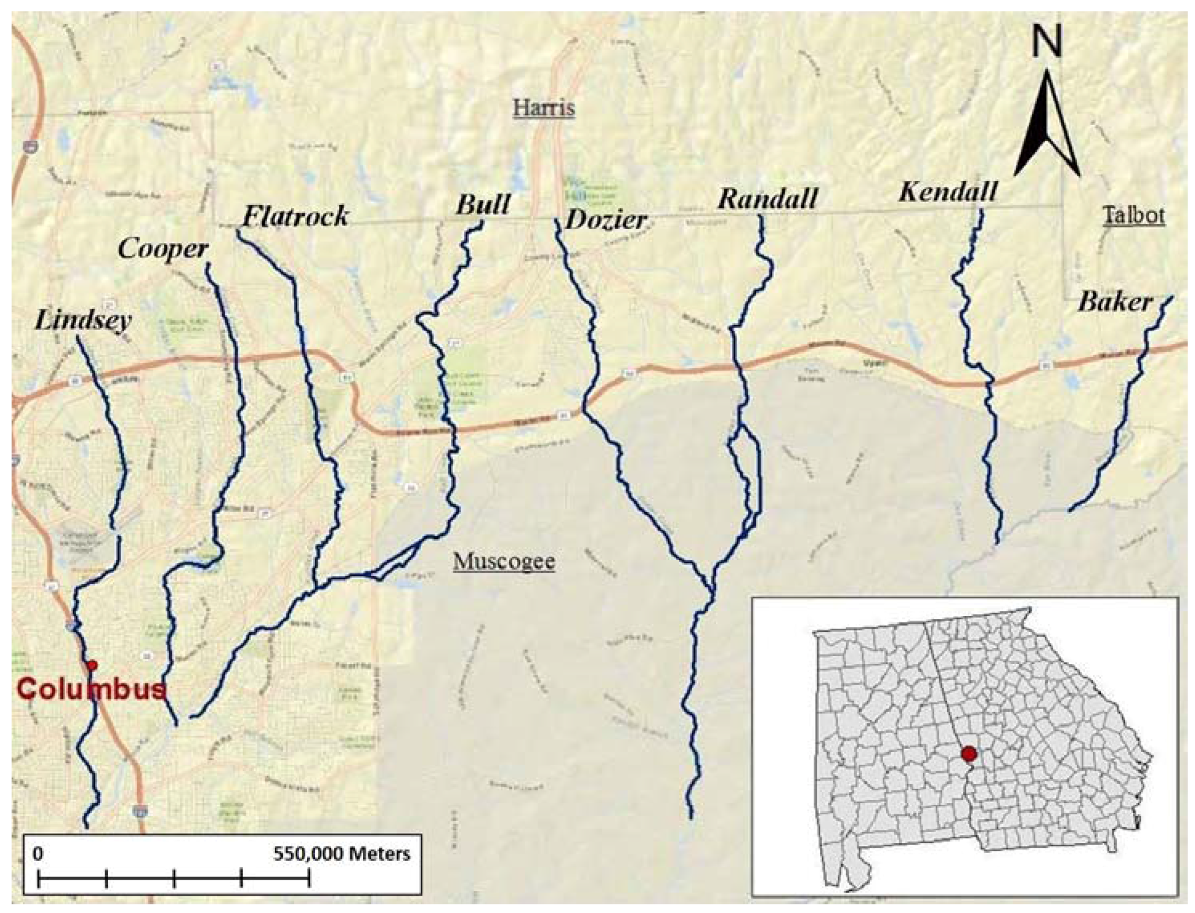
2.1. Study System and Defining Urbanization

Eight creeks (Lindsey, Cooper, Flatrock, Bull, Dozier, Randall, Kendall and Baker) within the Bull and Upatoi Creeks Watershed (within the Middle Chattahoochee basin, Muskogee County, Georgia) create a sampling design typical of urbanization studies located in western-central Georgia where the level of urbanization and land use change spatially along a gradient (e.g., [33,34,35]). Creeks are located north of Fort Benning and east of Columbus (Figure 1), flow southward and are considered Piedmont streams based upon stream characteristics and location [36].
To quantify urbanization and how it may correlate with decreased habitat quality and potential environmental stress, we defined urbanization (for later correlation with FA) by a set of chemical and land-use variables (Table 1). Chemical factors (total suspended solids and major ions, fluoride, chlorine, sulfate and orthophosphate) similar to those used in Georgia [37] were measured within each creek. Water samples from each creek were collected in acid-washed plastic sampling jars and transported to the Texas Research Institute for Environmental Studies (TRIES) Analytical Laboratory for analyses using standard methods for water and wastewater analysis [38]. Standard EPA methods were used to analyze orthophosphate (method #365.3) and fluoride, chlorine, and sulfate ions were quantified using ion chromatography (method #300.0). Water samples were also used to quantify total suspended solids (TSS). Common land-use characteristics generally associated with urbanization (Table 1) were analyzed using Geographic Information Systems software (ArcGIS 10.1, Environmental Systems Research Institute, Redlands, CA, USA) and included land-use, percent impervious surfaces, density of roads and human population density [21].

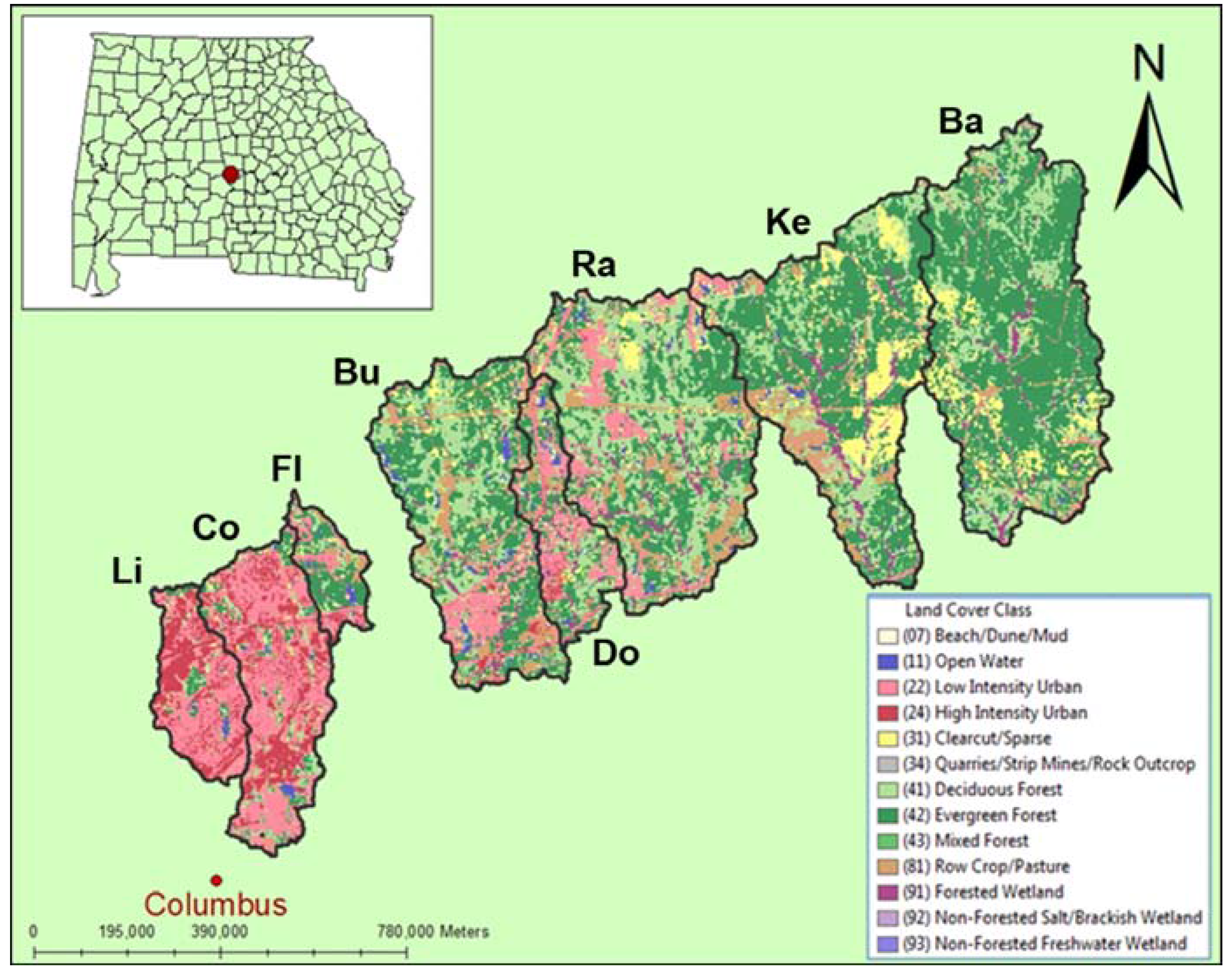
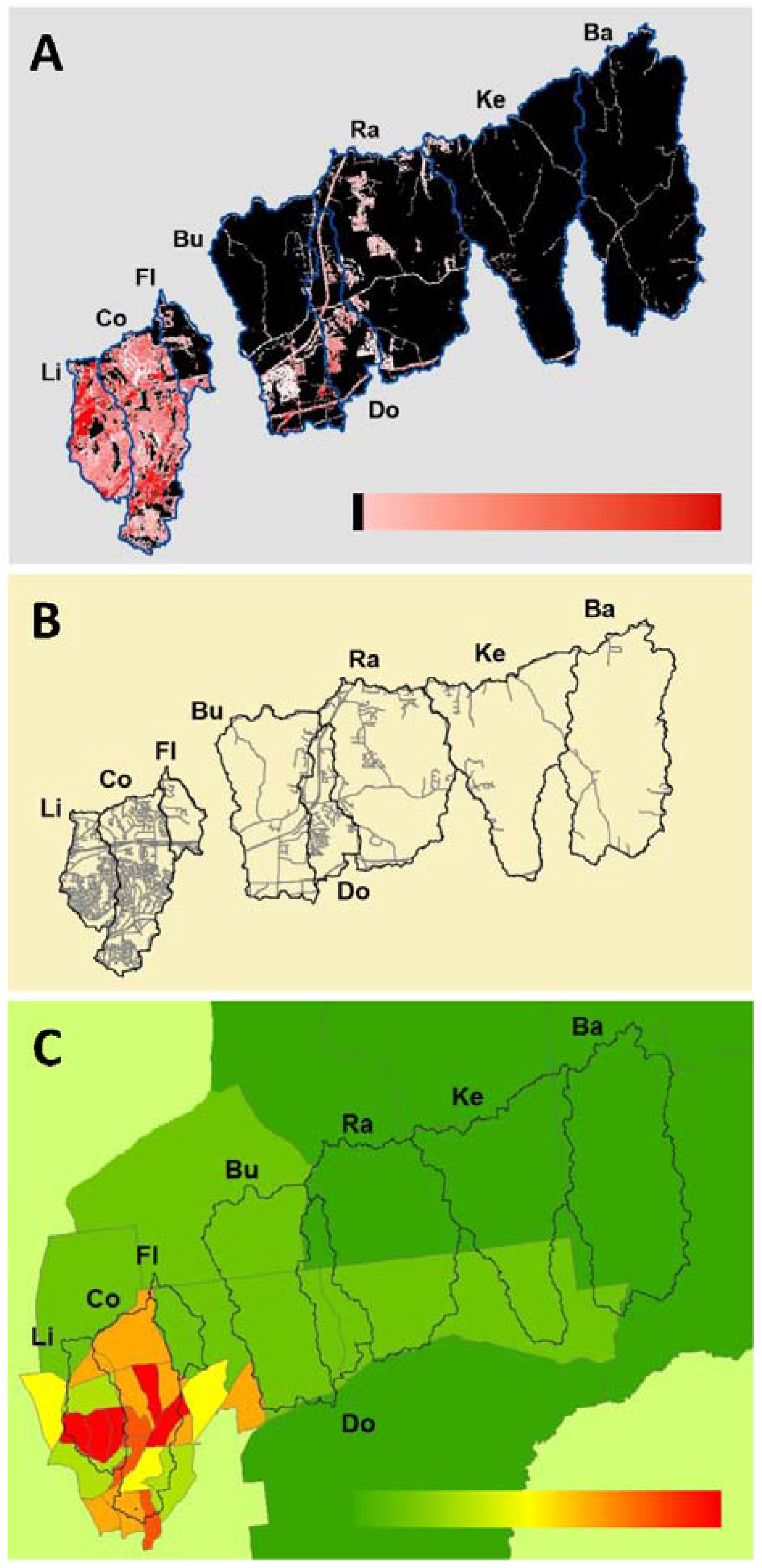
2.2. Land-Use Analyses

To quantify the land-use characteristics associated with each of the eight creeks within the watershed, we used the most recent land cover raster for the state of Georgia (file name: Georgia Land Use Trends Land Cover of Georgia 2008 from www.georgiaspatial.org). Using the North American Equal Area Conic projection for accuracy, we clipped the land cover raster to each of the creek basins. We then converted each of the clipped rasters to a polygon and used unique values to separate out each of the land-cover types that occur and calculated each area of the individual land-use type. Because similar land cover segments were listed separately within the attribute table based on their location, we quantified the total land cover area in square meters (m2) per type per basin. Once the area of each land cover type within each basin was quantified, they were summed to obtain an overall area for the basin. Overall area was used to calculate percentage total area represented by each land use type within each basin (Figure 2). Urban land-use is the percent land-use types which included Low Intensity Residential, High Intensity Residential, Clearcut/Sparse and Row Crop/Pasture. These were chosen based upon the Georgia land cover descriptions within the raster metadata (www.georgiaspatial.org).
Similarly, we used an impervious surface raster (file name: Ga. Land Use Trends Impervious Surface Cover 2008 from www.georgiaspatial.org) to quantify percent impervious surface and used the North American Equal Area Conic projection for accuracy. We clipped the land cover raster to each of the creek basins, and converted each of the clipped rasters to a polygon. We used unique values to separate out each of the percent impervious surface codes and calculated the area of each polygon of the impervious surface codes. We selected all impervious surface regions that were similarly coded within a basin and quantified the total area in m2 of each impervious surface code per basin (Figure 3a). There were a total of 20 impervious surface codes and each represented a five-increment percent imperviousness from 0% to 100% imperviousness. For example, the code 1 represents 1%–5% imperviousness and code 20 represents 96%–100%. We then summed all area values representing each impervious surface code to get a total area of the basin. Using this total area, we calculated percent total area represented by each code. Because values of 15% imperviousness and greater have been shown to cause water quality impairment [47], we summed the total area percentages for all codes (4–20) representing imperviousness above 15%.
To quantify road density (Figure 3b), we used a 2012 Georgia counties roads shapefile (file name: Roads and Highways; extent: Harris, Muscogee and Talbot Counties from www.georgiaspatial.org). We clipped the roads shapefile to each creek drainage basin and obtained all of the road segment lengths in meters (m) using a Georgia Universal Transverse Mercator (UTM) projection for accuracy. After obtaining the lengths of road segments, we summed the total length of all segments within each drainage to calculate total road length in kilometers (km).
We acquired data regarding 2010 population per block groups from the United States Census Bureau (2010 TIGER/Line Shapefiles from www.census.gov) and calculated population density within each drainage using the North American Albers Equal Area Conic projection for accuracy. We selected all census block groups that intersected each drainage. After clipping the total census block groups that intersected the basins, we calculated population density by dividing each block group population by each block group area that intersected each drainage and created a graduated colors map using the Natural Breaks classification method. We then summed the population density for each of the block groups that intersected each drainage to obtain the total population density associated with each drainage (Figure 3c). We used principal components analysis (PCA) to reduce the dimensionality of the combined GIS and water chemistry data. The resulting PCA axes were used as metrics of urbanization and correlated with measures of FA.

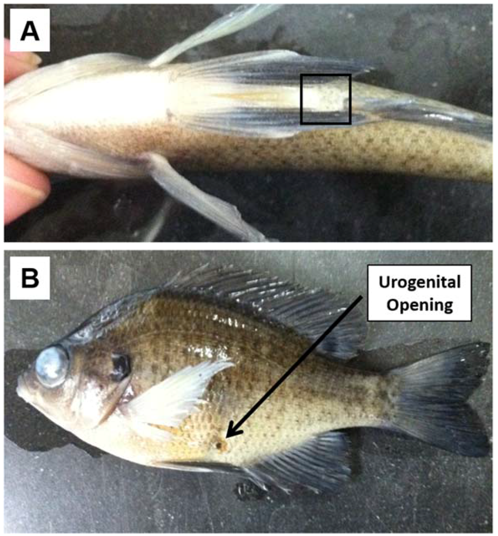
2.3. Fish Collection

A Previous survey of fishes (Permit # 29-WMB-01-147) was conducted in June 2001 and August 2002 [28] and served as the foundational data for investigating the effects of urbanization on biodiversity [28,29,30]. In October 2012, we collected only Lepomis specimens (Permit # 29-WJH-12-192) for this study using a backpack electrofisher until a minimum of 20 L. auritus and/or L. macrochirus were obtained from each of the eight creeks. Global Positioning System (GPS) coordinates were used to ensure fish were collected from the same localities sampled in both 2001 and 2002. All collections of fishes were euthanized and immediately fixed in 10% formalin for transport to the laboratory where they were washed, placed in 70% ethanol and catalogued for permanent archival in the Ichthyology Range of the Sam Houston State Vertebrate Museum.

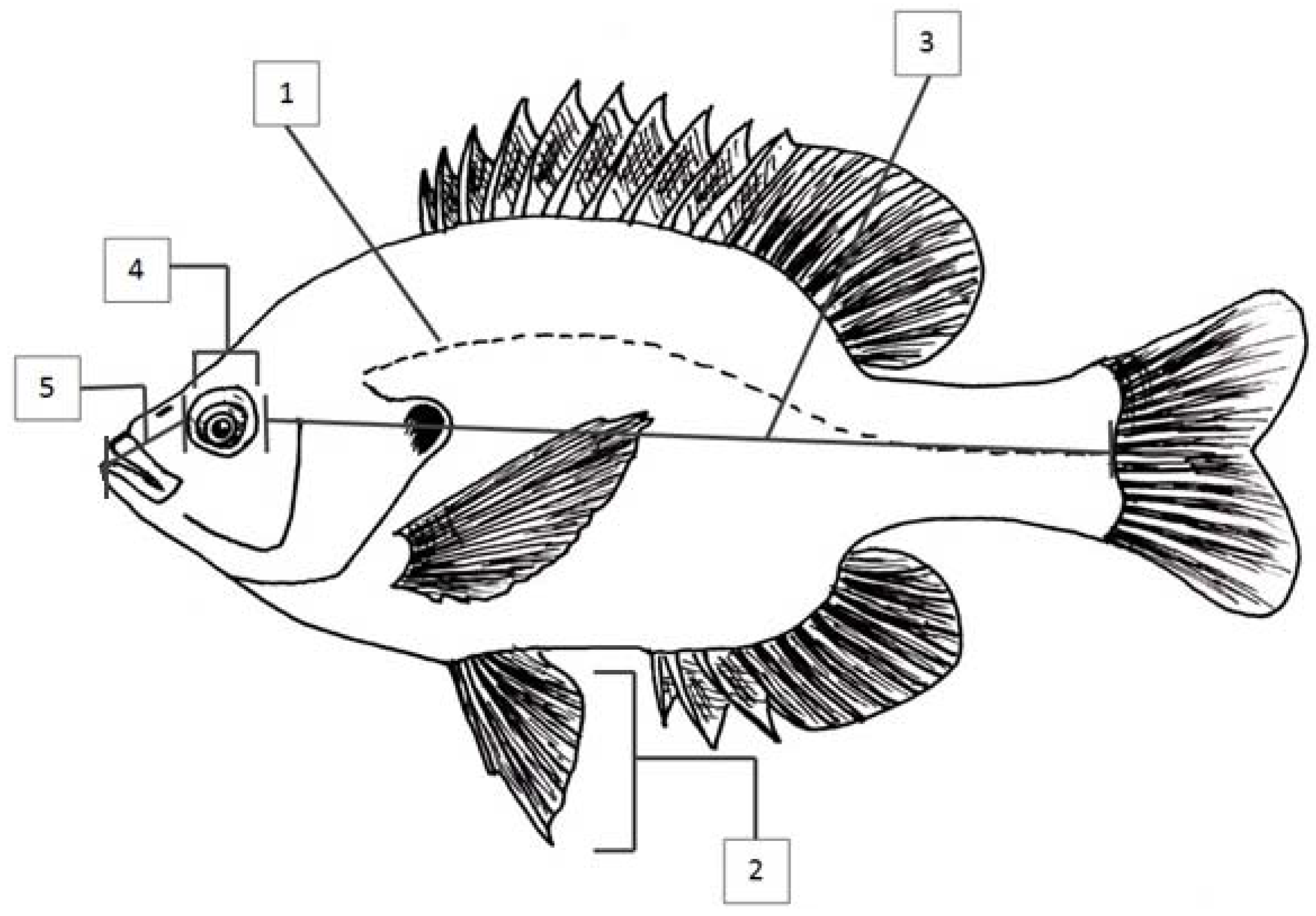
2.4. Metric and Meristic Analyses

We selected and quantified five paired bilateral characters (Figure 4) that are dichotomous and conserved between Lepomis species [27]. Preliminary results showed no significant responses and almost no variability in the FA of meristic characters among creeks. Thus, only metric characters were used here as these continuous (not discrete) data may offer more continuous variation for correlation with the urbanization gradient. Metric characters were measured to the nearest ±0.01 mm in triplicate on three different days allowing for assessment of measurement error (ME) [4].

2.5. Fluctuating Asymmetry Analysis

We followed the methods of Merila and Bjorklund in quantifying measurement error first and testing for differences in FA [48]. We used mixed-model repeated measures ANOVA (side of the fish served as the fixed factor and individual fish as the random repeated factor) to partition ME and test for differences among creeks. In this analysis, FA and ME are calculated from the mean square interaction (MSSxI) and the mean square within (MSwithin). To calculate FA, we subtracted the MSwithin from the MSSxI and divided that by the number of repeated measures (n = 3) [10]. To calculate ME, we divided the MSwithin by the newly calculated FA value. This assesses if ME is high in relation to FA, which indicates either a high occurrence of ME or low FA. After assessing ME, we tested for differences in FA among creeks using mixed-model ANOVA. Individual FA measures were then calculated as the signed mean differences between left and right measures (standardized by body size and averaged across the three replicate measures). Because all three metric measures (Figure 4) are potentially inter-correlated, a composite FA score for each individual was calculated by summing the three scaled (z-score) FA values for each individual. Individual composite FA scores were averaged for each creek and their mean values (±SE) were correlated with PCA axes (metrics of urbanization) to test hypotheses regarding associations between FA and urbanization.

3. Results

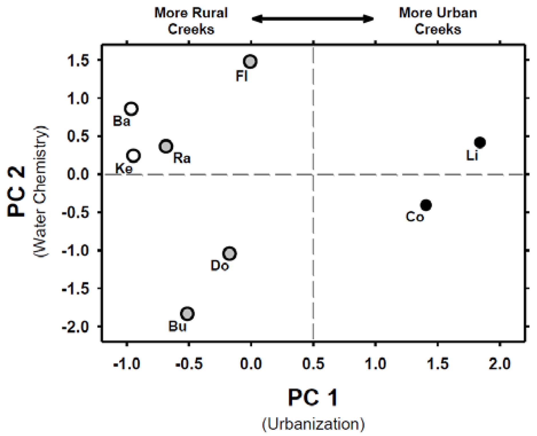
3.1. Land-Use Analyses and Chemical Factors of Urbanization

A summary of land-use and geospatial data (Table 2) using GIS quantified and illustrates a distinct urbanization gradient across the eight creeks (Lindsey, Cooper, Flatrock, Bull, Dozier, Randall, Kendall and Baker) within the Bull and Upatoi Creeks Watershed (Figure 3). Because water chemistry is related to the land-use characteristics of urbanization [37], chemical factors (total suspended solids and major ions, fluoride, chlorine, sulfate and orthophosphate) were quantified (Table 3).
All land-use and chemical factors were used in a principal component analysis (PCA) to investigate the relative similarities among creeks within multivariate space. The first principal component (PC1) explains 51% (eigenvalue 4.605) of the variation among creeks with respect to urbanization where impervious surface, land use, and population density loaded heaviest. The second principal component (PC2) explains 18% (eigenvalue 1.615) of the variation among creeks with total suspended solids (TSS), orthophosphate (negatively correlated), and sulfate (positively correlated) loading heaviest for water chemistry (Figure 5).

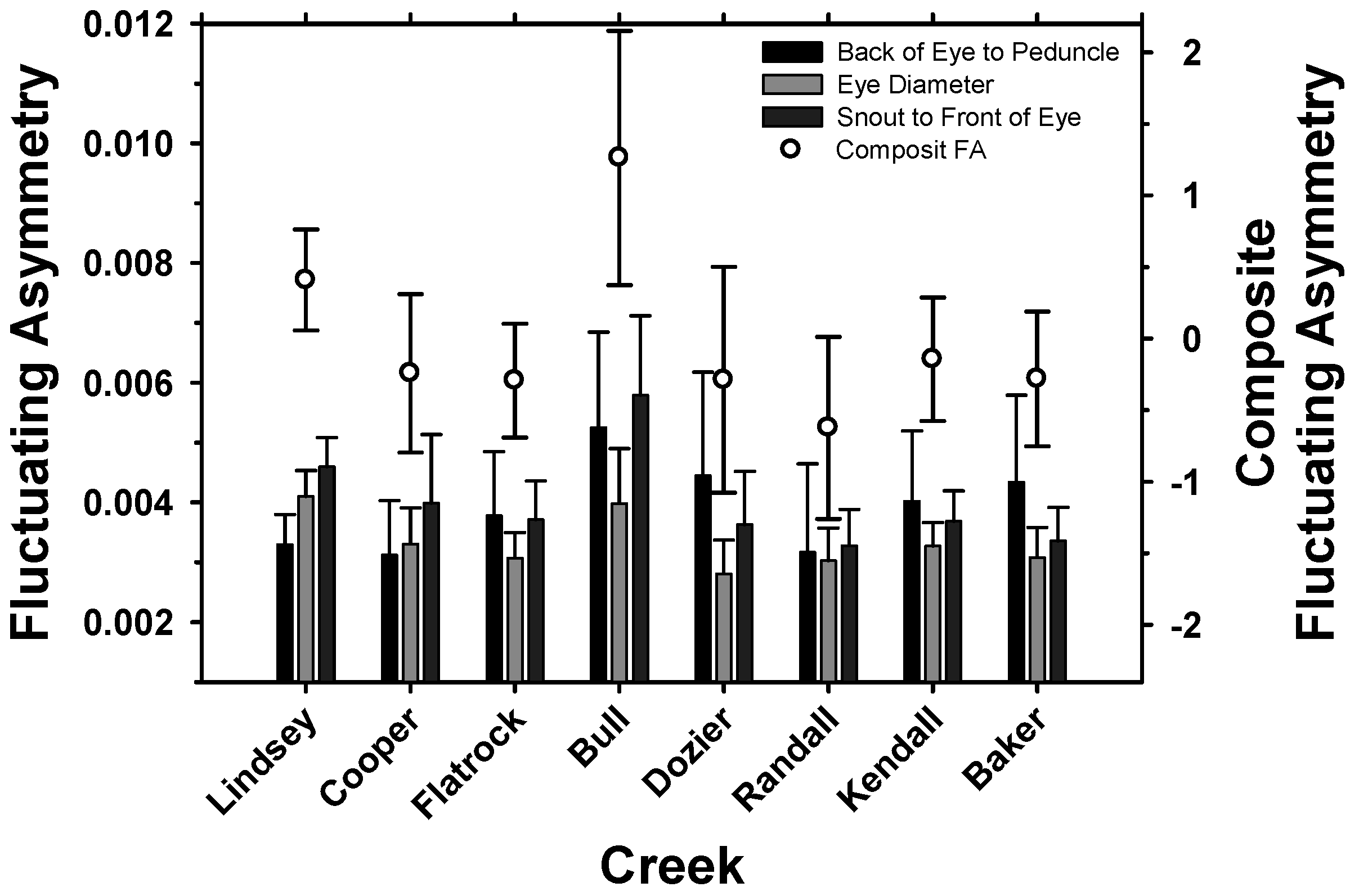
3.2. Fluctuating Asymmetry

Fluctuating asymmetry was quantified in 428 fishes (range = 22 to 119 fishes per creek; Table 4) collected in October 2012. Sampling of fishes within Bull, Dozier and Randall proved more difficult than other creeks but produced the minimum of 20 Lepomis specimens needed for investigating potential FA differences among creeks. We combined data from both L. auritus and L. macrochirus in a genus-level analysis because these species are phylogenetically [49] and eco-morphologically [50] similar. In addition, preliminary analyses using a mixed model ANOVA with side, individual and species as factors indicated no significant differences in FA responses between species for the three metric characters; eye to the caudal peduncle distance (F = 1.05, P = 0.304), eye diameter (F = 3.20, P = 0.094) and the front edge of the eye to the tip of the snout distance F = 0.384, P = 0.535). To ensure statistical power, this genus-level analysis was practical considering sampling restrictions and limitations (Permit # 29-WJH-12-192 and IACUC #12-09-25-1003-3-01). However, we do offer a cautionary note regarding the potential Yule–Simpson effect [51] when considering combined data.
Because metric characters and FA values may be positively influenced by body size [52], we analyzed the relationship between each metric character and body size. We found eye-peduncle distance (F1,426 = 24.3, r2 = 0.05, P < 0.001), eye diameter (F1,426 = 59.7, r2 = 0.12, P < 0.001), and eye-snout distance (F1,426 = 70.73, r2 = 0.14, P < 0.001) to be positively influenced by standard length. Prior to additional analyses of FA (and the calculation of composite scores), we corrected all FA values for the effects of scaling using the correction outlined in [52]. We found significant differences in FA of fishes among creeks (Table 5). All three FA measures were generally highest in Bull and Lindsey Creeks (Figure 6). Raw FA values by creek (mean difference between repeated L and R measures, standardized by body length) ranged from 0.0012 (Dozier) to 0.0018 (Lindsey) in eye diameter; 0.0025 (Cooper) to 0.0042 (Bull) in distance from front of eye to snout; and 0.0025 (Cooper) to 0.0042 (Bull) in distance from back of the eye to the caudal peduncle.

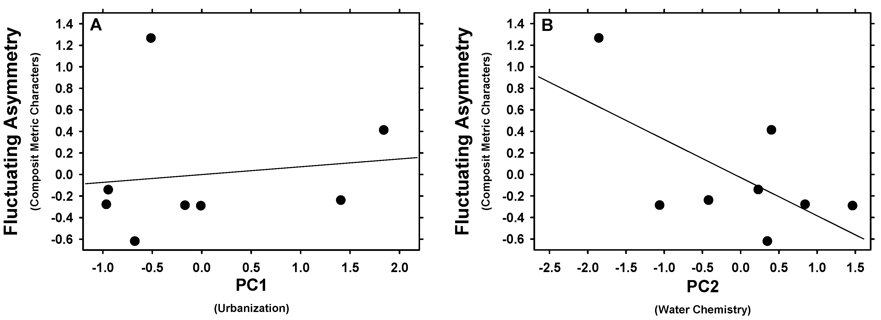
3.3. Fluctuating Asymmetry Related to Land-Use and Chemical Factors of Urbanization

Each creek’s PCA score for both principal components (PC1 = urbanization and PC2 = water chemistry) were regressed against its composite FA score to investigate if FA among individuals within a creek could be influenced by the land-use and chemical factors of urbanization (Figure 7). We found no relationship between urbanization (PC1) and composite FA (F = 0.130, P = 0.731). Environmental water chemistry did not regress with the composite FA (F = 3.501, P = 0.111) but showed a stronger trend than urbanization as a predictor (Table 6).

4. Discussion

We use GIS to spatially characterize urbanization and a land-use gradient (e.g., [33,34,35]) across eight creeks to investigate if increased urbanization would predict an increased degree of FA within resident fishes (Lepomis) of the Bull and Upatoi Creeks watershed. We predicted that fishes in Lindsey Creek, the most urban located within the urban center of Columbus, would have the highest FA and that the degree of FA would decrease predictably to the most rural, Baker Creek.
We found a distinct urbanization gradient among creeks with urban land-use, impervious surface, length of roads, and population density showing a clear decreasing trend eastward from Lindsey to Baker creek (Table 2, Figure 2 and Figure 3). The water chemistry associated with each creek drainage basin did not show such a clear decreasing tread except for chlorine ion, in which Bull Creek within the middle of the watershed had the lowest value (Table 3).
Both land-use and chemical factors associated with anthropogenic land-use and landscape scale processes can play a significant role in defining stream condition and thus create developmental stressors resulting in FA [23,53]. The fact that land-use and chemical factors were each associated with different PCA axes (each explaining a substantial amount of variation) indicates urbanization influences on creeks is more complex than linear gradients radiating away from population centers. Of the land-use and chemical factors investigated in this study, the PCA allowed us to characterize creeks in multivariate space and identify which land-use and chemical factors were important in defining differences among creeks (Figure 5). As expected, we found the two most urban creeks to be most similar in multivariate space and loaded in similar positions along the first principal component (PC1 = urbanization). Likewise, the most rural creeks (Kendall and Baker) loaded in similar positions with all other creeks being intermediate along PC1. Although the second principal component (PC2 = water chemistry) explained 18% of the variation among creeks, no trends are noticeable except that the intermediate creeks (Flatrock, Bull and Dozier) have the highest positive and negative PC2 scores (Figure 5). We should also note that although PC1 separates creeks along the eastward gradient (Figure 1), both the most urban and most rural creeks are most similar with respect to their PCS scores and therefore have similar total suspended solids (TSS), orthophosphate, and sulfate. Such similarity in environmental water chemistry occurs because both urban and agricultural based land-use can have similar impacts on water quality, habitat, and aquatic biota [53,54,55].
We found FA differences among creeks for two of the three metric characters (Table 5), but failed to show a linear relationship between an increasing urbanization gradient and increased FA (Table 6). Similar to the urbanization analyses, we found no significant relationships between FA and water chemistry. What might be of future interest is that we found significant relationships between urbanization and the standard deviation in eye-peduncle distance (F = 24.08, P = 0.003, r2 = 0.80) and environmental water chemistry and the standard deviation in the composite FA (F = 18.05, P = 0.005, r2 = 0.75). Different degrees of FA among individuals within in a population may identify environmental instability within both urban and rural creeks. Headwater streams are notoriously variable, especially in urban settings. Thus, one might expect varying strengths of FA signals from year to year. Fishes (Lepomis) are also long-live meaning fishes sampled within creeks are of different size (and thus age) and may be associated with degrees of FA resulting from a temporal aspect for the presences of environmental stressors within a system. Because FA is considered a population parameter as well as an individual parameter [1,6,10], individuals should have highly similar development of bilateral characters unless the system experience large shifts in environmental quality. Therefore, developmental differences among individuals within a creek may be strongly correlated with the temporal aspects of environment.
Other sources of differing degrees of FA among individuals in a population may be caused by temporal influences. In this study, each creek was sampled twice in 2012 and twice a decade prior. Again, Lepomis are long-lived species meaning that the group of individuals sampled are of different size classes (i.e., ages) and could have experienced different and unique developmental conditions during their particular time of development. Ideally, developmental periods are limited but our assumption here was that urbanization pressures would be ubiquitous through time. However, annual variability in temperature and water levels could impact a variety of stressors contributing to increase variability in dataset separated by 10 years of collection.
We were compelled to generate composite scores (see methods) for FA as all metric characters used here (Figure 4) are potentially inter-correlated. Although we regressed each metric character with urbanization and water chemistry for individual character comparison, we felt that a composite score of FA would provide a more comprehensive analysis. We plot the composite FA with the FA of individual metric characters and show how this composite FA compares to the group of metric per creek (Figure 6).
FA scores for individual metrics and the composite were highest in the most urban, Lindsey and Bull Creeks, (Figure 6). Furthermore, Lindsey Creek had the highest urbanization values (Table 2, Figure 3) while Bull Creek had one of the highest TSS and orthophosphate (Table 3). These two creeks with the highest FA (Figure 6) values also had the most extreme scores on each of these PCA axes (Lindsey = 1.84 on PC1, Bull = −1.8 on PC2; Figure 5). In regard to the others creeks, FA patterns along urbanization gradients were not as defined resulting in an inability to show significant effects of the urbanization gradient or water chemistry on the composite FA (Table 6, Figure 7).
Our land-use analyses show a strong urbanization gradient related to numerous land-use characteristics across creeks. The failure to show a relationship between FA and urbanization may be because the particular land-use in this study may not create adequate environmental stress to detect responses in FA. However, water chemistry may have a more direct influence on FA and may be a more powerful predictor of developmental stress than the indirect quantification of urbanization, even though urbanization might be linked to water quality within the aquatic system.
Numerous factors have been shown to increase FA and include inbreeding, nutrition, chemical contaminants and pH [27]. We show a significant difference in the degree of FA among the eight creeks studied (Table 5, Figure 6). The FA of metric characters were also found to be related to the land-use factor of population density and the chemical factors of TSS and orthophosphate potentially influenced by urbanization (Table 6, Figure 7). Our metrics of urbanization were not complete and there are likely other (unmeasured) factors that could contribute to FA in resident fishes. Small headwater streams like these are particularly variable environments where physiological tolerance to abiotic factors has been shown to play an important role in regulating populations [56]. Stream hydrology, chemistry and biota are dictated by factors that take place on varying spatial and scales, especially those taking place on regional and local levels [54,57]. Geomorphology and climate at a regional level and land-use and land cover at local levels are major drivers within a stream habitat.
Many studies have shown FA to be a reliable bioindicator of environmental stress (e.g., [12,13,14,15]). While some researchers have shown FA to be a poor indicator (e.g., [58]), community and assemblage indices may still predict urbanization (e.g., [28,29,34,39,47]). When considering potential bioindicators of environmental stress, specifically urbanization stress, community indices such as species diversity, richness, and total abundance seem to act as reliable bioindicators (e.g., [39]). Although the association between FA and the urbanization gradient among creeks was weak here, Martin and Lutterschmidt found that species richness and total abundance increased as urbanization decreased in this same study system [28].
The monitoring of changes in biodiversity is considered a powerful tool in evaluating environmental degradation and the health of aquatic ecosystems [59,60,61]. For example, Yoder et al. supported this idea that community indices seem to be highly sensitive indicators as when they showed that biologically sensitive fish species disappear at 0%–5% urban land-use and extreme loss of fish fauna occurs at greater than 15% urban land-use [62]. Additionally, it could be argued that the urbanization gradient treatment was not stressful enough to induce FA, but that seems unlikely because community level changes were detected. Community indices seem to be highly sensitive indicators as discussed by [62] where biologically sensitive fish species disappear at 0%–5% urban land-use and extreme loss of fish fauna occurs at greater than 15% urban land-use.
Related work in these same Georgia Peidmont streams [28,29] have documented how biodiversity may be affected by urbanization and potential environmental stress within this watershed. Martin and Lutterschmidt investigated the diversity of fishes within these same eight creeks within the Bull and Upatoi Creeks watershed and found that both species richness and total abundance correlated with distance from the urban center of Columbus, GA and percent urban land-use [28]. Additionally, a detailed survey of parasites sampled from 222 bluegill (Lepomis macrochirus) and 205 redbreast sunfish (Lepomis auritus) was conducted to provide a checklist for documenting the biodiversity of parasites within this watershed. The use of parasites as a bioindicator of ecosystem health is not novel [63,64] and may be particularly useful in environmental monitoring [65,66,67] and the monitoring of anthropogenic related pollutants [68]. Buck and Lutterschmidt further illustrated the link between host density, which is influenced by urbanization, and parasite abundance within this aquatic system [30].
Here, we investigate the use of FA as a potential biological indicator of the environmental stressors associated with an urbanization gradient associated with Columbus, Georgia. We found differences in environmental water chemistry among creeks across this urbanization gradient to be a better predictor of FA than urbanization. Future investigation of FA within this system may benefit from focusing on environmental water quality, microhabitat assessment, and changes in hydrology. These particular factors may be more meaningful for predicting responses in FA than characterizations of land-use along. Additionally, community level analyses of fishes may identify species with greater responses in FA that could better serve as biological indicators (e.g., [58,59,69]). Such community analyses of this system (e.g., [28]) have focused on the presence and absence of species and may benefit from investigations of differential responses in FA among the species within the fish community. Finally, FA may be observed in meristic and metric characters not typically quantified for study and extreme occurrence of FA in a single individual may prove meaningful biologically in identifying environmental stressors within a stream. Although not the most urban, we found Cooper Creek to be most impacted by urban disturbance related to road and population density (Table 2), debris, storm drainage, run-off and alteration of flow regime. Interestingly, one of the most dramatic and extreme examples of FA observed within this watershed was found in an individual (Figure 8) collected from Cooper Creek.

Acknowledgments

We thank Sidney M. Anderson, Riccardo A. Fiorillo, Laurianne Dent, Daniel S. Millican, Dennis K. Wasco and Kelbi D. Delaune for field assistance related to this research and acknowledge a scientific collector’s permit (# 29-WJH-12-192) issued by Georgia Dept. of Natural Recourses and the Sam Houston State University IACUC protocol (#12-09-25-1003-3-01) for research. We also thank Rachelle Smith, Operations Manager of the Texas Research Institute for Environmental Studies (TRIES) Analytical Laboratory, for water analyses. We thank Michael Homer and acknowledge the Texas Parks and Wildlife Department Inland Fisheries Office in Snook, Texas for support and use of field equipment including an electrofisher. We thank Don Albert and Falguni Mukherjee for their reviews and helpful guidance in the use of GIS to investigate and characterize land-use and acknowledge World Wide Web based information [70,71] used in our analyses. We acknowledge the assistance provided by Gordon A. Plishker and all personnel of the Texas Research Institute for Environmental Studies (TRIES) at Sam Houston State University. This work was supported in part by a grant from the Engineer Research and Development Center (ERDC) and the Civil Engineering Research Lab (CERL) of the US Army Corps of Engineers (ERDC-CERL Contract #DACA 42-00-C-0047) to William I. Lutterschmidt and we sincerely thank Hugh Westbury of the Strategic Environmental Research and Development Program (SERDP), Ecosystem Management Project (SEMP), and Harold (Hal) Balbach of the US Army ERDC and CERL for their sincere interest in and support of this project.

Author Contributions

W.I.L. conceived and designed the study, W.I.L. and S.L.M. performed field sampling and collection, S.L.M. sorted, identified, and cataloged all fishes for the museum, measured all meristic and metric characters for analyses, and conducted all GIS analyses, J.F.S. provide statistical expertise and analyzed fluctuating asymmetry data, W.I.L. provided graphical presentation of data, and W.I.L., S.L.M. and J.F.S. wrote and edited the manuscript.

Conflicts of Interest

The authors declare no conflict of interest.

References

  1. Moller, A.P.; Swaddle, J.P. Asymmetry, Developmental Stability, and Evolution; Oxford University Press: New York, NY, USA, 1997. [Google Scholar]
  2. Moller, A.P. Developmental stability and fitness: A review. Am. Nat. 1997, 149, 916–932. [Google Scholar]
  3. Zakharov, L.A. A measure of fluctuating asymmetry for a set of characters. Acta Zool. Fenn. 1992, 191, 37–77. [Google Scholar]
  4. Palmer, R.A. Fluctuating asymmetry analyses: A primer. In Developmental Stability: Its Origins and Evolutionary Implications; Markow, T.A., Ed.; Kluwer Academic Publishers: Dordrecht, The Netherlands, 1994; pp. 335–364. [Google Scholar]
  5. Lucentini, L.; Carosi, A.; Erra, R.; Giovinazzo, G.; Lorenzoni, M.; Mearelli, M. Fluctuating asymmetry in perch, Perca fluviatilia (Percidae) from three lakes of the Region Umbria (Italy) as a tool to demonstrate the impact of man-made lakes on developmental stability. Ital. J. Zool. 1998, 65, 445–447. [Google Scholar]
  6. Van Valen, L. A study of fluctuating asymmetry. Evolution 1962, 16, 125–142. [Google Scholar]
  7. Palmer, R.A. Waltzing with asymmetry. BioScience 1996, 46, 518–532. [Google Scholar] [CrossRef]
  8. Graham, J.H.; Shimizu, K.; Emlen, J.M.; Freeman, D.C.; Merkel, J. Growth models and the expected distribution of fluctuating asymmetry. Biol. J. Linn. Soc. 2003, 80, 57–65. [Google Scholar] [CrossRef]
  9. Hochwender, C.G.; Fritz, R.S. Fluctuating asymmetry in a Salix hybrid system: The importance of genetic versus environmental causes. Evolution 1999, 53, 408–416. [Google Scholar] [CrossRef]
  10. Palmer, R.A.; Strobeck, C. Fluctuating asymmetry: Measurement, analysis, and patterns. Annu. Rev. Ecol. Evol. Syst. 1986, 17, 391–421. [Google Scholar] [CrossRef]
  11. Palmer, R.A.; Strobeck, C. Fluctuating asymmetry as a measure of developmental stability: Implications of non-normal distributions and power of statistical tests. Acta Zool. Fennica 1992, 191, 57–72. [Google Scholar]
  12. Siegel, P.; Siegel, M.I.; Krimmer, E.C.; Doyle, W.J.; Barry, H. Fluctuating asymmetry as an indicator of the stressful prenatal effects of D9-tetrahydrocannabinol in the laboratory rat. Toxicol. Appl. Pharm. 1977, 42, 339–344. [Google Scholar] [CrossRef]
  13. Hardersen, S. The role of behavioural ecology of damselflies in the use of fluctuating asymmetry as a bioindicator of water pollution. Ecol. Entomol. 2000, 25, 45–53. [Google Scholar] [CrossRef]
  14. Bonada, N.; Williams, D.D. Exploration of the utility of fluctuating asymmetry as an indicator of river condition using larvae of the caddisfly Hydropsyche morose (Trichoptera: Hydropsychidae). Hydrobiologia 2002, 481, 147–156. [Google Scholar] [CrossRef]
  15. Seixas, L.B.; Neves Dos Santos, A.F.G.; Neves Dos Santos, L. Fluctuating asymmetry: A tool for impact assessment on fish populations in a tropical polluted bay, Brazil. Ecol. Indic. 2016, 71, 522–532. [Google Scholar] [CrossRef]
  16. Tull, J.C.; Brussard, P.F. Fluctuating asymmetry as an indicator of environmental stress from off-highway vehicles. J. Wildl. Manag. 2006, 71, 1944–1948. [Google Scholar] [CrossRef]
  17. Lajus, D.; Rainer, K.; Brix, O. Fluctuating asymmetry and other parameters of morphological variation of eelpout Zoarces viviparus (Zoarcidae, Teleostei) from different parts of its distributional range. Sarsia 2003, 88, 247–260. [Google Scholar] [CrossRef]
  18. Estes, E.C.; Katholi, C.R.; Angus, R.A. Elevated fluctuating asymmetry in eastern mosquitofish (Gambusia holbrooki) from a river receiving paper mill effluent. Environ. Toxicol. Chem. 2006, 25, 1026–1033. [Google Scholar] [CrossRef] [PubMed]
  19. Pickett, S.T.A.; Cadenasso, M.L.; Grove, J.M.; Nilon, C.H.; Poutay, R.V.; Zipperer, W.C.; Constanza, R. Urban ecological systems: Linking terrestrial ecology, physical, and socioeconomic components of metropolitan areas. Annu. Rev. Ecol. Syst. 2001, 32, 127–157. [Google Scholar] [CrossRef]
  20. Weller, B.; Ganzhorn, J.U. Carabid beetle community composition, body size, and fluctuating asymmetry along an urban-rural gradient. Basic Appl. Ecol. 2004, 5, 193–201. [Google Scholar] [CrossRef]
  21. Hahs, A.K.; McDonnell, M.J. Selecting independent measures to quantify Melbourne’s urban-rural gradient. Landsc. Urban Plan. 2006, 78, 435–448. [Google Scholar] [CrossRef]
  22. Duh, J.; Shandas, V.; Chang, H.; George, L.A. Rates of urbanization and the resiliency of air and water quality. Sci. Total Environ. 2008, 400, 238–256. [Google Scholar] [CrossRef] [PubMed]
  23. Poff, N.L.; Allan, J.D.; Bain, M.B.; Karr, J.R.; Prestegaard, K.L.; Richter, B.D.; Sparks, R.E.; Stromberg, J.C. The natural flow regime. BioScience 1997, 47, 769–784. [Google Scholar] [CrossRef]
  24. Graham, J.H.; Emlen, J.M.; Freeman, C.D. Developmental stability and its applications in ecotoxicology. Ecotoxicology 1993, 2, 175–184. [Google Scholar] [CrossRef] [PubMed]
  25. Valentine, D.W.; Soule, M. Effect of p,p’-DDT on developmental stability of pectoral fin rays in the grunion, Leuresthes tenius. Fish. Bull. 1973, 71, 921–926. [Google Scholar]
  26. Ames, L.J.; Felley, J.D.; Smith, M.H. Amounts of asymmetry in Centrarchid fish inhabiting heated and nonheated reservoirs. Trans. Am. Fish. Soc. 1979, 108, 489–495. [Google Scholar] [CrossRef]
  27. Allenbach, D.M. Fluctuating asymmetry and exogenous stress in fishes: A review. Rev. Fish Biol. Fish. 2011, 21, 355–376. [Google Scholar] [CrossRef]
  28. Martin, S.M.; Lutterschmidt, W.I. A checklist to the common Cyprinid and Centrachid fishes of the Bull and Upatoi Creeks Watershed of Georgia with a brief glimpse of correlative urban influences and land use. Southeast. Nat. 2013, 12, 769–780. [Google Scholar] [CrossRef]
  29. Anderson, S.M.; Fiorillo, R.A.; Cook, T.J.; Lutterschmidt, W.I. Helminth parasites of two species of Lepomis (Osteichthyes: Centrarchidae) from an urban watershed and their potential use in environmental monitoring. Ga. J. Sci. 2015, 73, 123–135. [Google Scholar]
  30. Buck, J.C.; Lutterschmidt, W.I. Parasite abundance decrease with host density: Evidence of the encounter-dilution effect for a parasite with a complex life cycle. Hydrobiology 2017, 784, 201–210. [Google Scholar] [CrossRef]
  31. Deal, B. Ecological urban dynamics: The convergence of spatial modelling and sustainability. Build. Res. Inf. 2001, 29, 381–393. [Google Scholar] [CrossRef]
  32. Wang, Y.; Choi, W.; Deal, B.M. Long-term impacts of land-use change on non-point source pollutant loads for the St. Louis metropolitan area, USA. Environ. Manag. 2005, 35, 194–205. [Google Scholar] [CrossRef] [PubMed]
  33. Callender, E.; Rice, K.C. The urban environmental gradient: Anthropogenic influences on the spatial and temporal distributions of lead and zinc in sediments. Environ. Sci. Technol. 2000, 34, 232–238. [Google Scholar] [CrossRef]
  34. Helms, B.S.; Feminella, J.W. Detection of biotic responses to urbanization using fish assemblages from small streams of western Georgia, USA. Urban Ecosyst. 2005, 8, 39–57. [Google Scholar] [CrossRef]
  35. Styers, D.M.; Chappelka, A.H. Urbanization and atmospheric deposition: Use of bioindicators in determining patterns of land-use change in western Georgia. Water Air Soil Pollut. 2009, 200, 371–386. [Google Scholar] [CrossRef]
  36. Griffith, G.E.; Omernik, J.M.; Comstock, J.A.; Lawrence, S.; Martin, G.; Goddard, A.; Hulcher, V.J.; Foster, T. Ecoregions of Alabama and Georgia; US Geological Survey: Reston, VA, USA, 2001.
  37. Crim, J.F. Water Quality Changes Across an Urban-Rural Land Use Gradient in Streams of the West Georgia Piedmont. Master’s Thesis, Auburn University, Auburn, AL, USA, December 2007. [Google Scholar]
  38. Clesceri, L.S.; Greenberg, A.E.; Eaton, A.D. (Eds.) Standard Methods for the Examination of Water and Wastewater, 20th ed.; American Public Health Association: Washington, DC, USA, 1998.
  39. Paul, M.J.; Meyer, J.L. Streams in the urban landscape. Annu. Rev. Ecol. Syst. 2001, 32, 333–365. [Google Scholar] [CrossRef]
  40. Schoonover, J.E.; Lockaby, B.G. Land cover impacts on stream nutrients and fecal coliform in the lower Piedmont of west Georgia. J. Hydrol. 2006, 331, 371–382. [Google Scholar] [CrossRef]
  41. Camargo, J.A.; Alonso, A. Ecological and toxicological effects of inorganic nitrogen pollution in aquatic ecosystems: A global assessment. Environ. Int. 2006, 32, 831–849. [Google Scholar] [CrossRef] [PubMed]
  42. Hubbard, R.K.; Sheridan, J.M. Streamflow water quality in the Georgia coastal plain. In Proceedings of the 1989 Georgia Water Resources Conference, Athens, GA, USA, 16–17 May 1989.
  43. Dickerson, B.R.; Vinyard, G.L. Effects of high levels of the total dissolved solids in Walker lake, Nevada, on survival and growth of Lahontan cutthroat trout. Trans. Am. Fish. Soc. 1999, 128, 507–515. [Google Scholar] [CrossRef]
  44. Biggs, T.W.; Dunne, T.; Martinelli, L.A. Natural controls and human impacts on stream nutrient concentrations in a deforested region of the Brazilian Amazon basin. Biogeochemistry 2004, 68, 227–257. [Google Scholar] [CrossRef]
  45. Theobald, D.M. Placing exurban land-use change in a human modification framework. Front. Ecol. Environ. 2004, 2, 139–144. [Google Scholar] [CrossRef]
  46. Jones, J.A.; Swanson, F.J.; Wemple, B.C.; Snyder, K.U. Effects of roads on hydrology, geomorphology, and disturbance patches in stream networks. Conserv. Biol. 2000, 14, 76–85. [Google Scholar] [CrossRef]
  47. Klein, R.D. Urbanization and stream quality impairment. Water Resour. Bull. 1979, 15, 948–963. [Google Scholar] [CrossRef]
  48. Merila, J.; Bjorklund, M. Fluctuating asymmetry and measurement error. Syst. Biol. 1995, 44, 97–101. [Google Scholar] [CrossRef]
  49. Roe, K.J.; Harris, P.M.; Mayden, R.L. Phyolgenetic relationships of the genera of North American sunfishes and basses (Percoidei: Centrarchidae) as evidenced by the mitochondrial cytochrome b gene. Copeia 2002, 2002, 897–905. [Google Scholar] [CrossRef]
  50. Collar, D.C.; O’Meara, B.C.; Wainright, P.C.; Near, T.J. Piscivory limits diversification of feeding morphology in Centrarchid fishes. Evolution 2009, 63, 1557–1573. [Google Scholar] [CrossRef] [PubMed]
  51. Yule, G.U. Notes on the theory of association of attributes in statistics. Biometrika 1903, 2, 121–134. [Google Scholar] [CrossRef]
  52. Pertoldi, C.; Kristensen, T.N. A new fluctuating asymmetry index, or the solution for the scaling effect? Symmetry 2015, 7, 327–335. [Google Scholar] [CrossRef]
  53. Allan, J.D. Landscapes and riverscapes: The influence of land use on stream ecosystems. Annu. Rev. Ecol. Evolut. Syst. 2004, 35, 257–284. [Google Scholar] [CrossRef]
  54. Richards, C.; Johnson, L.B.; Host, G.E. Landscape-scale influences on stream habitats and biota. Can. J. Fish. Aquat. Sci. 1996, 53, 295–311. [Google Scholar] [CrossRef]
  55. Roy, A.H.; Rosemond, A.D.; Paul, M.J.; Leigh, D.S.; Wallace, J.B. Stream macroinvertebrate response to catchment urbanization (Georgia, USA). Freshw. Biol. 2003, 48, 329–346. [Google Scholar] [CrossRef]
  56. Matthews, W.J. Physiochemical tolerance and selectivity of stream fishes as related to their geographic ranges and local distributions. In Community and Evolutionary Ecology of North American Stream Fishes; University of Oklahoma Press: Norman, OK, USA, 1987; pp. 111–120. [Google Scholar]
  57. Wang, L.; Lyons, J.; Kanehl, P.; Bannerman, R. Impacts of urbanization on stream habitat and fish across multiple spatial scales. Environ. Manag. 2001, 28, 255–266. [Google Scholar] [CrossRef]
  58. Bjorksten, T.; David, P.; Pomiankowski, A.; Fowler, K. Fluctuating asymmetry of sexual and nonsexual traits in stalk-eyed flies: A poor indicator of developmental and genetic quality. J. Evol. Biol. 2001, 13, 89–97. [Google Scholar] [CrossRef]
  59. Karr, J.R. Assessment of biotic integrity using fish communities. Fisheries 1981, 6, 21–27. [Google Scholar] [CrossRef]
  60. Fausch, K.D.; Lyons, J.; Karr, J.R.; Angermeier, P.L. Fish Communities as Indicators of Environmental Degradation. Am. Fish. Soc. Symp. 1990, 8, 123–144. [Google Scholar]
  61. Cookson, N.; Schorr, M.S. Correlation of watershed housing density with environmental conditions and fish assemblages in a Tennessee ridge and valley stream. J. Freshw. Ecol. 2009, 24, 553–561. [Google Scholar] [CrossRef]
  62. Yoder, C.O.; Miltner, R.J.; White, D. Assessing the status of aquatic life designated uses in urban and suburban watersheds. In National Conference on Retrofit Opportunities for Water Resource Protection in Urban Environment, Chicago, IL, USA, 9–12 February 1998; pp. 16–28.
  63. Adams, S.M. Status and use of biological indicators for evaluating the effects of stress on fish. J. Parasitol. 1990, 70, 466–474. [Google Scholar]
  64. Marcogliese, D.J. Parasites of the superorganism: Are they indicators of ecosystem health? Int. J. Parasitol. 2005, 35, 705–716. [Google Scholar] [CrossRef] [PubMed]
  65. Lafferty, K.D. Environmental parasitology: What can parasites tell us about human impacts on the environment? Parasitol. Today 1997, 13, 251–256. [Google Scholar] [CrossRef]
  66. Kennedy, C.R. Freshwater fish parasites and environmental quality: An overview and caution. Parassitologia 1997, 39, 249–254. [Google Scholar] [PubMed]
  67. Sures, B. Environmental parasitology: Relevancy of parasites in monitoring environmental pollution. Trends Parasitol. 2004, 20, 170–177. [Google Scholar] [CrossRef] [PubMed]
  68. Khan, R.A.; Billiard, S.M. Parasites of winter flounder (Pleuronectes americanus) as an additional bioindicator of stress-related exposure to untreated pulp and paper mill effluent: A 5-year field study. Arch. Environ. Contam. Toxicol. 2007, 52, 243–250. [Google Scholar] [CrossRef] [PubMed]
  69. Karr, J.R.; Yant, P.R.; Faush, K.D.; Schlosser, I.J. Spatial and temporal variability of the index of biotic integrity in three Midwestern streams. Trans. Am. Fish. Soc. 1987, 116, 1–11. [Google Scholar] [CrossRef]
  70. Georgia Spatial Data Infrastructure. Georgia GIS Clearinghouse: Map Data and Aerial Photography. Georgia Spatial Web, 2011. Available online: www.georgiaspatial.org (accessed on 23 July 2013).
  71. United States Census Bureau TIGER/Line Shapefiles and TIGER/Line Files. United States Census Bureau Web. Available online: http://www.census.gov (accessed on 23 July 2013).
Figure 1. Map of the eight creeks (Lindsey, Cooper, Flatrock, Bull, Dozier, Randall, Kendall and Baker) located within Muscogee County. Creeks are located within the Bull and Upatoi Creeks Watershed where the degree of urbanization decreases eastward from Lindsey Creek located in the Columbus urban center to Baker being the most rural.
Symmetry 08 00124 g001
Figure 2. Map of land cover types within each drainage basin for all eight creeks: Lindsey (Li), Cooper (Co), Flatrock (Fl), Bull (Bu), Dozier (Do), Randall (Ra), Kendall (Ke) and Baker (Ba).
Symmetry 08 00124 g002
Figure 3. Map showing relative differences in: (A) impervious surface; (B) total road length; and (C) population density within each drainage basin for all eight creeks (see Figure 2 for creek codes). Scales are shown for (A) where black is 0% and red is 100% impervious service; and (B) where green is low and red is high population density.
Symmetry 08 00124 g003
Figure 4. Meristic and metric dichotomous characters that are conserved between Lepomis species [27] were selected and quantified. Meristic characters: (1) pored lateral line scales; and (2) pelvic fin rays were not used in analyses. Metric characters included: (3) distance from the back edge of the eye to the caudal peduncle; (4) eye diameter; and (5) the front edge of the eye to the tip of the snout and were used in analyses as these continuous (not discrete) data offered bilateral variation.
Symmetry 08 00124 g004
Figure 5. Principal components analysis (PCA) showing the relative similarities among creeks within multivariate space. PC1 (principal component) explains 51% (eigenvalue 4.605) of the variation among creeks with respect to urbanization where impervious surface, land use, and population density loaded heaviest. PC2 explains 18% (eigenvalue 1.615) of the variation among creeks with total suspended solids (TSS), orthophosphate (negatively correlated), and sulfate (positively correlated) loading heaviest for water chemistry. Black, gray, and white points represent most urban, intermediate and most rural creeks, respectively.
Symmetry 08 00124 g005
Figure 6. Graphs of FA (absolute value of the mean difference between sides |R-L|) scores among creeks for metric characters: (3) distance from the back edge of the eye to the caudal peduncle; (4) eye diameter; and (5) the front edge of the eye to the tip of the snout (Figure 4). Composite FA scores are shown by open circles with error bars. Error bars show 95% confidence intervals.
Symmetry 08 00124 g006
Figure 7. The relationship between the composite fluctuating asymmetry scores and the: (A) urbanization; and (B) water chemistry PCA scores. See Table 6 for summary statistics.
Symmetry 08 00124 g007
Figure 8. Fish (L. auritus) specimen collected (6 October 2012) from Cooper Creek showing major deviation in symmetry for the location of the urogenital opening. The urogenital opening is not present along the sagittal plane (A) but rather located on the left lateral side of the body; (B) Such a specimen is referred to as a major phenodeviant. This specimen is archived in the ichthyology range of the Sam Houston State Vertebrate Museum (SHSVM #1375).
Symmetry 08 00124 g008
Table 1. Chemical and land-use factors used for quantifying urbanization, their potential effects and supporting citations.
Chemical FactorCause and EffectsCitations
Orthophosphates, fluoride, chlorine and sulfatesFertilizers, cleaning agents, human and food wastes, wastewater treatments.
Acidification, increased primary production, eutrophication and changes in nutrient cycling.
[38,39,40,41]
Total suspended solidsIncreased erosion, decreased water quality.
Fish growth and survival, nutrient cycling.
[39,42,43]
Land-Use FactorPotential EffectsCitations
Urban land use changeChanges in fish assemblage, water quality, stream landscapes, nutrient cycling etc.[21,34,44,45]
Impervious surfacesInfluence water quality, water quantity, hydrology, nutrient cycling, flood pulse index, increased down cutting, changes in riparian zone, etc.[19,34,39]
Road densityChanges in riparian areas (increased erosion) and stream geomorphology, flow, flooding, discharge, increased disturbance, etc.[21,39,45,46]
Population densityChanges in water quality, water quantity, nutrient cycling, etc.[19,44,45]
Table 2. Percent urban land use, percent urban (greater than 15% imperviousness) impervious surface, total length of road within each of the eight creek drainage basins, and total population density of census block groups that intersect with each of the eight creek drainage basins.
CreekPercent Urban Land UsePercent Urban Impervious SurfaceTotal Length (km) of RoadPopulation Density (People/km2)
Lindsey90.0581.1187.19,922.6
Cooper84.2167.91154.914,832.5
Flatrock46.1923.5919.22,488.2
Bull30.828.1357.61,048.5
Dozier47.4222.5052.6265.1
Randall29.407.4567.1158.6
Kendall27.542.8534.9145.1
Baker14.341.3026.7121.1
Table 3. Results of chemical factors associated with creek from most urban to most rural. Figure 1 shows the relative location of each creek from the urban center of Columbus, Georgia.
CreekTSS (total suspended solids) (mg/L)Fluoride (ppm)Chlorine (ppm)Sulfate (ppm)Orthophosphate (mg/L)
Lindsey018.845211.21725.70660.0470
Cooper20.13829.21433.93000.0120
Flatrock20.19529.93356.16060.0030
Bull40.12082.69622.87270.0650
Dozier519.11366.87032.29440.0090
Randall10.08895.20483.38050.0038
Kendall00.47754.28052.00650.0045
Baker00.22753.84764.41780.0130
Table 4. Summary for the number of redbreast sunfish (L. auritus) and bluegill (L. macrochirus) collected within the Bull and Upatoi Creeks Watershed by species and creek. Fish were collected in October 2012 (Permit # 29-WJH-12-192) using a backpack electrofisher.
CreekL. auritusL. macrochirusTotal
Lindsey8633119
Cooper173653
Flatrock362359
Bull19524
Dozier18422
Randall28129
Kendall432972
Baker361450
Total283145428
Table 5. Estimates of FA (fluctuating asymmetry) and ME (measurement error) from the mixed-model Analysis of Variance (ANOVA) testing for significant difference in FA among creeks. The three metric characters (Figure 4) included: (3) distance from the back edge of the eye to the caudal peduncle; (4) eye diameter; and (5) the front edge of the eye to the tip of the snout measured to the nearest ±0.01 mm. Both the FA of eye diameter (P = 0.013) and eye-snout distance (P = 0.012) of fishes significantly different among creeks. FA equals Mean Squares interaction (SxI) minus the Mean Squares within divided by the number of repeated measures which equaled three. ME equals Mean Squares within divided by FA.
Metric CharacterMS (SxI)MS (Within)FAMEFP
Eye-Peduncle Distance (3)0.277780.085390.096170.085391.200.299
Eye Diameter (4)0.043320.012830.015240.012832.5690.013
Eye-Snout Distance (5)0.046570.013760.016410.013762.5970.012
Table 6. Simple linear regression results for pairs of PCA (principal component analysis) scores of each principal component (PC1 = urbanization and PC2 = water chemistry) regressed against the FA and variation in FA (i.e., standard error, SE) of each metric character and the composite FA by creek (n = 8). Results indicate that the land-use and chemical factors can predict an urbanization response in FA and the variation in FA for some of the metric characters of fishes. The F statistic (F), probability (P) and the amount of variation in FA or the standard error of FA that can be explained by the urbanization gradient among creeks (r2) is shown with degrees of freedom = 1, 6.
PC1 UrbanizationPC2 Water Chemistry
FA Metric CharacterFPr2FPr2
Eye-Peduncle Distance2.5920.1590.3022.6040.1580.303
Eye Diameter1.7380.2350.2250.5920.4710.090
Eye-Snout Distance0.4460.5290.0694.2230.0860.413
Composite FA0.1300.7310.0213.5010.1110.368

