Similarity and a Duality for Fullerenes

Abstract

Fullerenes are molecules of carbon that are modeled by trivalent plane graphs with only pentagonal and hexagonal faces. Scaling up a fullerene gives a notion of similarity, and fullerenes are partitioned into similarity classes. In this expository article, we illustrate how the values of two important fullerene parameters can be deduced for all fullerenes in a similarity class by computing the values of these parameters for just the three smallest representatives of that class. In addition, it turns out that there is a natural duality theory for similarity classes of fullerenes based on one of the most important fullerene construction techniques: leapfrog construction. The literature on fullerenes is very extensive, and since this is a general interest journal, we will summarize and illustrate the fundamental results that we will need to develop similarity and this duality.

1. Introduction

Throughout this paper, we consider a fullerene to be a trivalent plane graph $\Gamma =\left(V,E,F\right)$ where all of the faces are pentagonal or hexagonal. It follows directly from Euler’s formula that all but exactly 12 faces are hexagons. We often consider the dual to the fullerene, the geodesic dome ${\Gamma }^{*}$, which is the triangulation of the sphere with 12 vertices of degree-five and the remaining of degree-six. For every pentagon, f, in a fullerene Γ, there is a corresponding degree-five vertex, $f^{*}$, in ${\Gamma }^{*}$. By a face path between two pentagons in a fullerene, we look to the dual and consider the faces identified with the vertices of a path between corresponding degree-five vertices. We say that two pentagons, f and g, are neighbors in Γ if no other degree-five vertices in ${\Gamma }^{*}$ lie on the shortest path between $f^{*}$ and $g^{*}$. If we let Λ be the hexagonal tessellation of the plane and ${\Lambda }^{*}$ be the triangular tessellation of the plane, then these tessellations form a framework upon which we can map our fullerene/geodesic dome structures. Just as the geodesic dome is the dual of a fullerene, ${\Lambda }^{*}$ is the dual of $\Lambda .$

Given two neighboring pentagons, f and g, we form a local coordinate system in ${\Lambda }^{*}$ for the union of all shortest paths in ${\Gamma }^{*}$ joining $f^{*}$ and $g^{*}$, where $f^{*}$ is taken to be the origin and $g^{*}$ is in the first quadrant. The straight line, l, in ${\Lambda }^{*}$ through $f^{*}$ is said to be the x-axis if the wedge formed by l and the ray through the origin that is 60° counterclockwise from l contains $g^{*}$. We say this ray is the y-axis. The unit length in this coordinate system is the edge length in ${\Lambda }^{*}$. 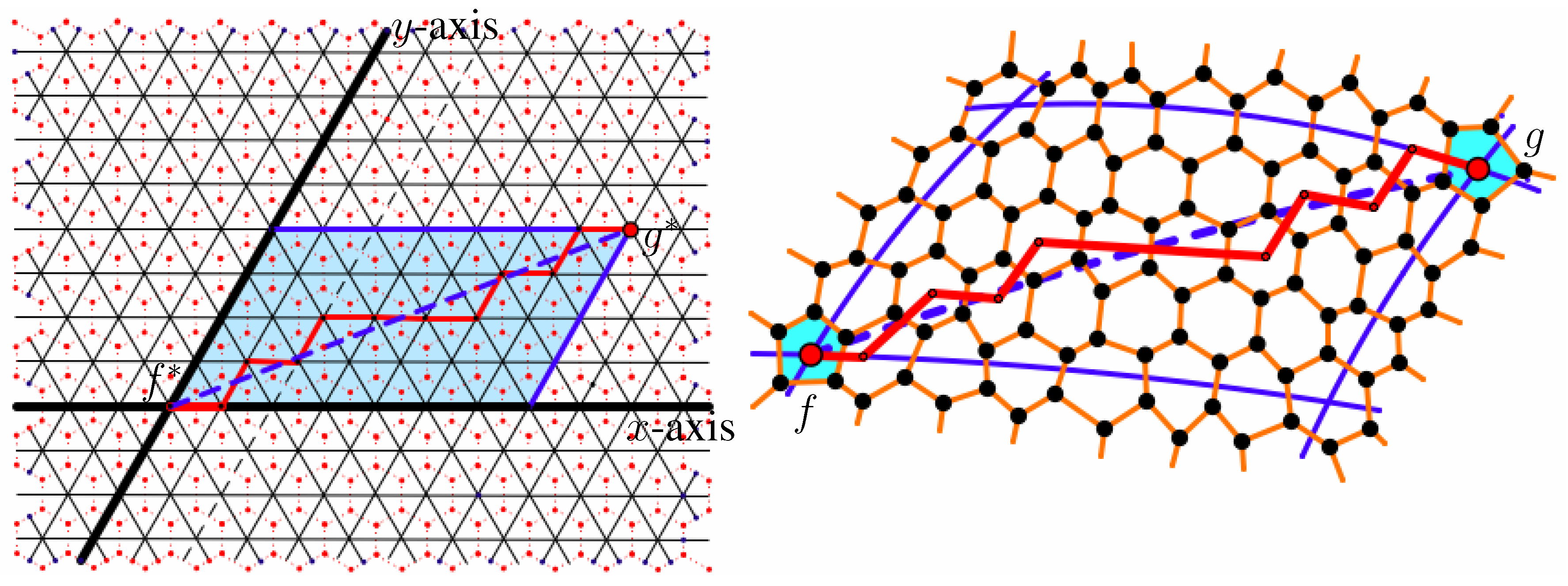For every pair of faces of Λ, we define a segment of Λ to be the straight line segment in two-space joining the centers of the two faces. The Coxeter coordinates of this segment are then the coordinates of $g^{*}$ in this coordinate system. An example of the coordinate system is shown in Figure 1. One should note that the Coxeter coordinates remain the same, if the roles of f and g are reversed; also, the Coxeter coordinates are reversed for the segment joining f and g in the mirror image of Γ. In the case when either coordinate is zero, we simply assign the segment a single Coxeter coordinate, $\left(p\right)$.

Figure 1. The coordinates of the segment shown are $(7,4)$.

Figure 1. The coordinates of the segment shown are $(7,4)$.

We say that two segments, $(a_1,b_1)$ and $(a_2,b_2)$ are adjacent if the segments each have one endpoint exiting a particular face, f. Similarly, we say a set of segments form a string if each segment is adjacent to two other segments with the exception of the first and last segments in the string, which are adjacent to only one.

We often want to consider the length of a segment σ with endpoints v and w. We define the length of σ, denoted $\left|\sigma \right|$, to be the distance between the endpoints in the graph Λ. There are several ways to interpret this length. The first method is to let $\left|\sigma \right|=p+q$ when $\sigma =(p,q)$. Using this definition of length, it is clear that there are many distinct Coxeter coordinates that all have the same length. For example, $(2,2)$ and $\left(4\right)$ both have length four; however, $(2,2)$ is shorter geometrically than $\left(4\right).$ To account for this in [3], Graver defines $\left|\left(p,q\right)\right|=p+q+\left|\frac{p-q}{p+q+1}\right|$. This way, segments are first divided into groups by graph theory distance and then within these groups are ordered by geometric distance.

For two adjacent segments, we define the angle between them to be $\theta \in \left\{1,2,3,4\right\}$, where θ is the number of vertices of the pentagon that lies between them when traversed counterclockwise or equivalently the number of edges in the corresponding geodesic dome. In cases where the segment has a single Coxeter coordinate of the form $\left(p\right)$, the segment coincides directly with an edge of the geodesic dome. As such, to avoid ambiguity, we say that the segment contributes $\frac{1}{2}$ to each of the angles on either side of the segment. As we are considering these angles around a pentagon, it follows that the angles around any vertex in the graph of a fullerene sum to five.

We now define an auxiliary graph in which the vertices represent the pentagonal faces of Γ. The edges in this new graph correspond to segments joining neighboring pentagons of $\Gamma .$ Using the length formula, $\left|\left(p,q\right)\right|=p+q+\left|\frac{p-q}{p+q+1}\right|$, we assign a weight to all of the edges in the auxiliary graph. The signature graph is the subgraph of the auxiliary graph that includes the edges that lie on some shortest spanning tree. The signature is the signature graph in which the edges are labeled with the Coxeter coordinates, and angles between edges are labeled by the measure of the angles between adjacent segments. The signature uniquely determines the fullerene or corresponding geodesic dome, as is shown in [3]. We denote the signature of a fullerene, Γ, to be $\mathcal{S}=\left(\Theta ,\theta ,c\right)$ in which Θ is the signature graph, θ is the function that represents the angle labels around each vertex and c is the function that represents the Coxeter coordinates of each segment.

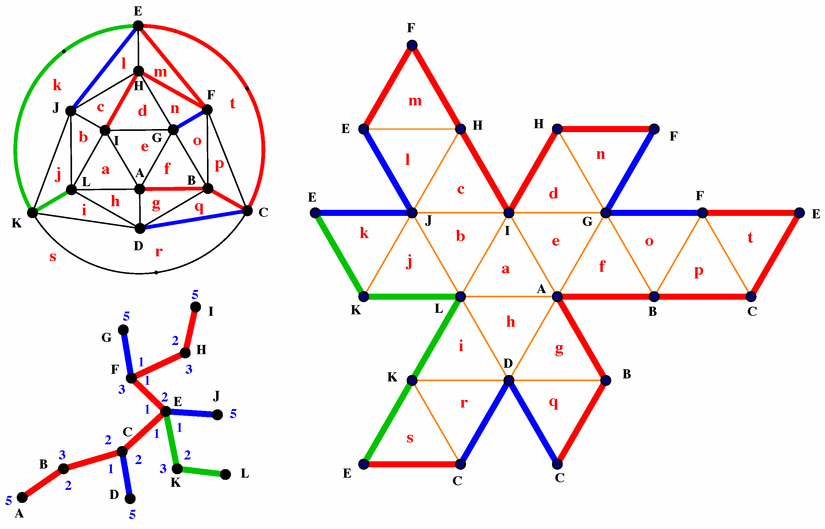
To create a flat map of the fullerene, we cut along the segments that correspond to one of the shortest spanning trees and unfold the fullerene. It was shown in [3] that fullerenes can be unfolded in this manner with no overlapping portions. An example of such a flat map is shown in Figure 2 along with the corresponding shortest spanning tree and the signature graph.

Figure 2. Fullerene on an icosahedron. Top right: signature graph of fullerene. Bottom left: one possible shortest spanning tree. Right: flat map of fullerene.

Figure 2. Fullerene on an icosahedron. Top right: signature graph of fullerene. Bottom left: one possible shortest spanning tree. Right: flat map of fullerene.

2. Similarity

Let ${\Gamma }_1$ and ${\Gamma }_2$ be two fullerenes and $\alpha \in \mathbb{Q}$. We say ${\Gamma }_1$ and ${\Gamma }_2$ are similar if the signature graphs are isomorphic with equal corresponding angles and the coordinates of the corresponding segments in the signature are proportional. More precisely, for every pair of corresponding segments, $\left(p_1,q_1\right)$ and $(p_2,q_2)$, we have $\frac{p_1}{p_2}=\frac{q_1}{q_2}=\alpha$, where α is the constant of proportionality. If the Coxeter coordinates of the segments in a fullerene have no common divisors, then we say Γ is reduced. Since all of the coordinates must be integers, it follows that all similar fullerenes are proportionally scaled versions of the reduced signature where the constant of proportionality is an integer. 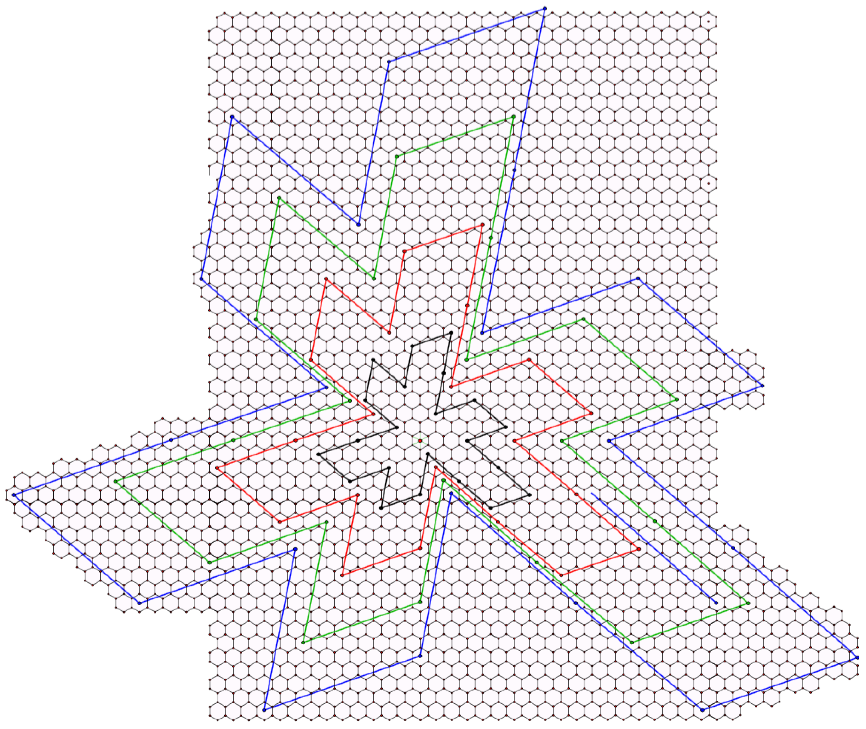If we consider two non-reduced signatures, then the constant of proportionality can be a fixed rational constant, α, given that scaling each coordinate by α yields integer coordinates. In Figure 3, we have taken the flat map of the reduced icosahedral fullerene with Coxeter coordinates $(2.1)$ (shown in black) and dilated its boundary by the factors of 2 (red), 3 (green) and 4 (blue). The center of the dilation is the red point in the center of the central hexagon.

Figure 3. Dilating the flat map of a fullerene.

Figure 3. Dilating the flat map of a fullerene.

Lemma 1. Let O be the center of a hexagon in Λ. Dilating by an integer factor from O sends centers of faces onto centers of faces.

Proof. In our coordinate system for Λ, the centers of faces all have integer coordinates. Consider the center of a face given by coordinates $(a,b)$. Let Λ be fixed. Dilating the plane about O by $m\in \mathbb{Z}$ will send $(a,b)$ to $(ma,mb)$, which is the center of a new face. ☐

Lemma 2. Let O be the center of a hexagon in Λ. Dilating by an integer factor from O sends segments to segments.

Proof. Let Λ be fixed and $(a,b)$ be the coordinates of the segment that connects faces f and g. By Lemma 1, we know that the dilation sends the centers of f and g to the centers of new faces, which we denote by $mf$ and $mg$. As such, the dilated segment connects the centers of $mf$ and $mg$ and has coordinates $(ma,mb)$. ☐

Lemma 3. Let O be the center of a hexagon in Λ. Dilating adjacent segments by an integer factor from O yields adjacent segments with the same angle measure.

Proof. Dilations preserve angle measures. ☐

Theorem 4. Let $\mathcal{S}$ be the signature of a reduced fullerene Γ. If all Coxeter coordinates in $\mathcal{S}$ are multiplied by $m\in \mathbb{Z}$, then the resulting structure is the signature of a new fullerene.

Proof. Consider a spanning tree of Γ with edge and angle labels. Scaling the spanning tree by multiplying all edge coordinates by m yields a new labeled tree. We take a flat map of the original spanning tree, and using the three lemmas, we see that the image of the boundary of the flat map under dilation by m corresponds to the dilated spanning tree. This shows that we do indeed have the flat map of a new fullerene.

We now want to show that all other distances in Γ are also dilated by m.

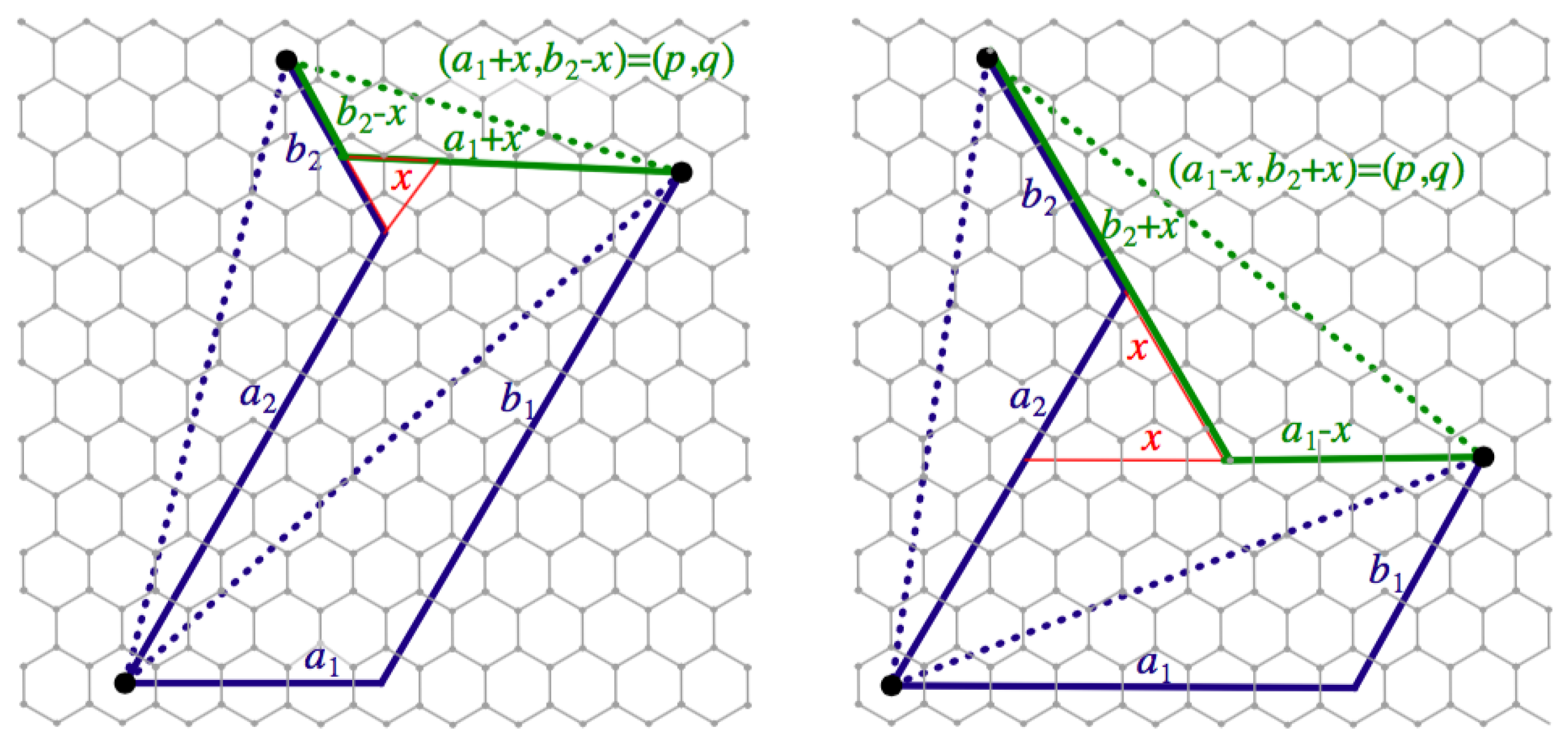
We will proceed by induction. We begin by considering the base case of two adjacent segments. Let $(a_1,b_1)$ and $(a_2,b_2)$ be the two adjacent segments in ${\Gamma }_1$, and let θ be the included angle. Therefore, the corresponding segments have Coxeter coordinates $(m{a}_1,m{b}_1)$ and $(m{a}_2,m{b}_2)$ in ${\Gamma }_2$ with the same included angle. Let $(p,q)$ be the Coxeter coordinates of the non-included side in ${\Gamma }_1$ represented by the green segment in Figure 4. We show that the non-included side in ${\Gamma }_2$ has length $m\left|\left(p,q\right)\right|.$ For this proof, it suffices to use the definition of length given by $\left|\right(a,b\left)\right|=a+b$.

Case 1: $\theta =1$

$\left|\left(p,q\right)\right|=\left|\left(a_1-x,b_2+x\right)\right|=a_1+b_2$ as is illustrated in Figure 4. There are two cases shown: one in which $a_2<b_1$ and another in which $a_2>b_1.$ Both cases yield the same length for $(p,q)$. The subsequent cases of larger angle measures are constructed similarly.

$\left|\left(mp,mq\right)\right|=\left|\left(m{a}_1-y,m{b}_2+y\right)\right|=m{a}_1+m{b}_2=m(a_1+b_2)=m\left|\left(p,q\right)\right|$

Figure 4. Calculating the length of the third side for adjacent segments with an enclosed angle of one.

Figure 4. Calculating the length of the third side for adjacent segments with an enclosed angle of one.

Case 2: $\theta =2$

$a_1\le b_2$: $\left|\left(p,q\right)\right|=\left|\left(a_1+a_2+b_1,b_2-a_1\right)\right|=b_1+b_2+a_2$

$\left|\left(mp,mq\right)\right|=\left|\left(m{a}_1+m{a}_2+m{b}_1,m{b}_2-m{a}_1\right)\right|=m{b}_1+m{b}_2+m{a}_2=m\left(b_1+b_2+a_2\right)=m\left|\left(p,q\right)\right|$

$a_1\ge b_2$: $\left|\left(p,q\right)\right|=\left|\left(a_1+a_2-x+b_1,x\right)\right|=a_1+a_2+b_1$

$\left|\left(mp,mq\right)\right|=\left|\left(m{a}_1+m{a}_2-y+m{b}_1,y\right)\right|=m{a}_1+m{a}_2+m{b}_1=m\left(a_1+a_2+b_1\right)=m\left|\left(p,q\right)\right|$

Case 3: $\theta =3$

$\left|\left(p,q\right)\right|=\left|\left(a_1+a_2,b_1+b_2\right)\right|=a_1+a_2+b_1+b_2$

$\left|\left(mp,mq\right)\right|=\left|\left(m{a}_1+m{a}_2,m{b}_1+m{b}_2\right)\right|=m{a}_1+m{a}_2+m{b}_1+m{b}_2=m\left(a_1+a_2+b_1+b_2\right)=m\left|\left(p,q\right)\right|$

Case 4: $\theta =4$

$\left|\left(p,q\right)\right|=\left|\left(a_2+x,b_1-x\right)\right|=b_1+a_2$

$\left|\left(mp,mq\right)\right|=\left|\left(m{a}_2+y,m{b}_1-y\right)\right|=m{b}_1+m{a}_2=m(b_1+a_2)=m\left|\left(p,q\right)\right|$

As such, scaling the components of the Coxeter coordinates by m also scales the non-included side by m. It follows that the length of the non-included side remains greater than both of the included sides. Hence, the two sides remain in the signature, while the non-included one remains excluded. Therefore, the claim holds for the base case.

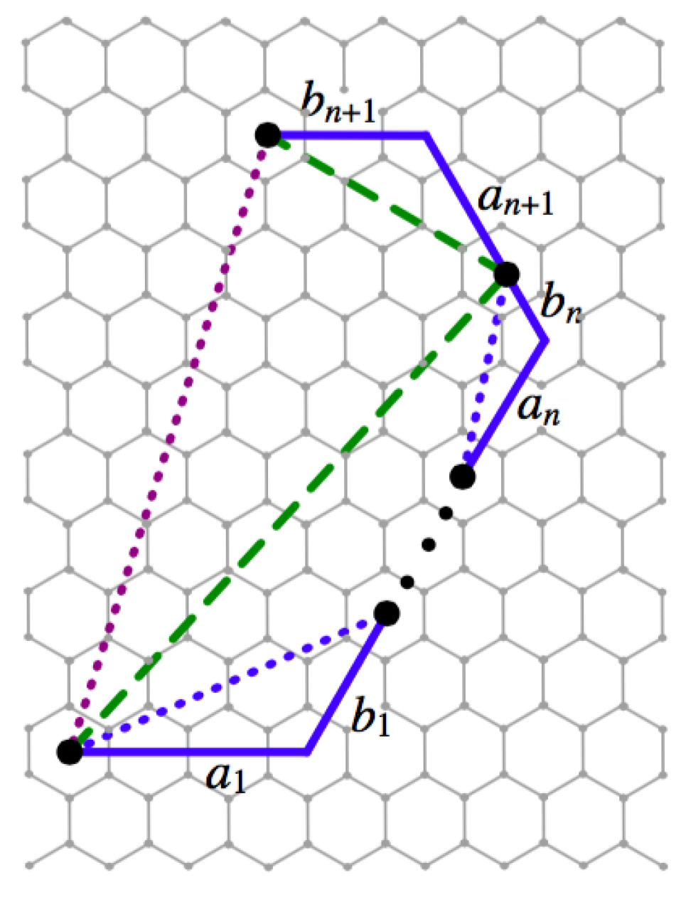
Now, assume the claim holds for a string of adjacent segments of length n in ${\Lambda }_1$, noticing that $n\le 11$ by the definition of a fullerene. Then, the length of the segment connecting the end points of the n adjacent segments is m-times larger than its corresponding segment in ${\Lambda }_1.$ Looking at a string of $n+1$ adjacent segments, the first n have an included segment that is scaled by m, and we scale the $\left(n+1\right)$ segment by m, as well. We can see in Figure 5 that once the endpoints of the string of n segments has been shown to be scaled by m, then by the base case, this gives us that the claim holds for our string of length $n+1.$ The signature of any fullerene can be viewed as a union of strings with a length of at most 11. As the claim holds for all such strings, we conclude that the resulting scaled graph is the signature of a new fullerene.  ☐

Figure 5. The string of $n+1$ adjacent segments can be reduced to the base case of two segments.

Figure 5. The string of $n+1$ adjacent segments can be reduced to the base case of two segments.

3. Leapfrog Fullerenes

Given any fullerene $\Gamma =\left(V,E,F\right)$ where $\left|V\right|=n$, we can construct a fullerene ${\Gamma }^{\prime }=\left(V^{\prime },E^{\prime },F^{\prime }\right)$, where $\left|V^{\prime }\right|=3n$ using a method called the leapfrog construction, which is shown in Figure 6. To construct the leapfrog fullerene of Γ, an extra vertex is added to the center of each face of $\Gamma .$ These new vertices are connected with all of the vertices surrounding the face in which the new vertex lies; in the figure, this is shown with the pink edges. This new graph has triangular faces and vertices of degrees five and six and, therefore, is a geodesic dome. The dual of this new graph (shown in green) is then a fullerene, and one easily checks that it has $3n$ vertices. We say that any fullerene that could have been constructed in this manner is a leapfrog fullerene. We note that in the construction of ${\Gamma }^{\prime }$, each pentagonal face is in the center of a pentagonal face of Γ. Hence, there is a natural correspondence between the pentagons of ${\Gamma }^{\prime }$ and the pentagons of Γ.

Figure 6. Green edges show the result of the leapfrog construction on original blue faces.

Figure 6. Green edges show the result of the leapfrog construction on original blue faces.

The Coxeter coordinates of a segment joining a pair of pentagons in Γ changes as we move to the segment joining the corresponding pair of pentagons in ${\Gamma }^{\prime }$. To compute this change, we apply the leapfrog operation to Λ, giving ${\Lambda }^{\prime }$, the leapfrog tessellation, and then compute the Coxeter coordinates of the representative segments in both Λ and ${\Lambda }^{\prime }$. The results of these computations are recorded in the next lemma.

Lemma 5. Let σ be a segment in Λ, and let ${\Lambda }^{\prime }$ the leapfrog tessellation. The Coxeter coordinates of σ in ${\Lambda }^{\prime }$ are calculated from the Coxeter coordinates of σ in Λ as described in the following table:

$$\begin{array}{ccccc}\Lambda coordinates& \left(p+r,p\right)& \left(p,p+r\right)& \left(p,p\right)& \left(r\right)\\ {\Lambda }^{\prime } coordinates& \left(r,r+3p\right)& \left(r+3p,r\right)& \left(3p\right)& \left(r,r\right)\end{array}$$

Since the coordinates change, the resulting fullerene need not be similar to the original. It follows that the signature of the two need not be isomorphic, as can be seen in Figure 7. In the figure, the dark purple segments represent segments in the original fullerene that are included in the signature, and the pink segments represent the coordinates of the non-included side. The dark green and light green segments represent the coordinates of the segments when the leapfrog construction is applied. As can be seen in the figure, the two dark green sides are no longer shorter than the light green side, so the signature is altered.

Figure 7. Leapfrog construction may change the signature of a fullerene.

Figure 7. Leapfrog construction may change the signature of a fullerene.

It follows from Lemma 5 that the Coxeter coordinates of segments in a leapfrog fullerene are always congruent mod three. We say the signature of fullerene is of the leapfrog type if the coordinates of each segment in the signature are congruent modulo three, and it was proven in [4] that a fullerene is a leapfrog fullerene if and only if its signature is of the leapfrog type. Many of the properties of leapfrog fullerenes were worked out in [1]. We will consider one of the more important properties of leapfrog fullerenes in a later section.

4. Duality

The collection of all fullerenes can be partitioned into equivalence classes of similar signatures. By looking at the structure of the most reduced signature in the class, we can separate the equivalence classes into those of the leapfrog type and those of the non-leapfrog type. In a class of the leapfrog type, the reduced fullerene is a leapfrog, and hence, all fullerenes in the class are leapfrog. In a non-leapfrog-type class, the reduced fullerene is not a leapfrog fullerene. It is important to note that there are leapfrog fullerenes within classes of the non-leapfrog type, namely when the scaling factor, m, is a multiple of three.

Performing the leapfrog construction twice yields a fullerene in the similarity class of the original one. From this, we have a duality between similarity classes in which the dual of a leapfrog type fullerene is one of the non-leapfrog type. We call this the leapfrog dual.

Theorem 6. Dual similarity classes cannot both be of the leapfrog type.

Proof. Let Γ be a reduced leapfrog fullerene, and let ${\Gamma }^{\prime }$ be its leapfrog dual. Assume by way of contradiction that both fullerenes are in leapfrog-type classes. Since the Coxeter coordinates of the segments in the signature of Γ must be congruent modulo three, it follows that the Coxeter coordinates are all of the form $\left(p+r,p\right)$, $\left(p,p+r\right)$, $\left(p,p\right)$ or $\left(r\right)$, where $r=3s$ for some $s\in \mathbb{N}$, but s and p are not a multiple of three. By the previous lemma, we get the following table.

$$\begin{array}{ccccc}\Lambda \mathrm{coordinates}& \left(p+3s,p\right)& \left(p,p+3s\right)& \left(p,p\right)& \left(3s\right)\\ {\Lambda }^{\prime } \mathrm{coordinates}& \left(3s,3s+3p\right)& \left(3s+3p,3s\right)& \left(3p\right)& \left(3s,3s\right)\end{array}$$

Reducing ${\Gamma }^{\prime }$ by dividing through by three results in non-leapfrog fullerene. As such, both Γ and ${\Gamma }^{\prime }$ cannot be in the leapfrog-type classes. ☐

5. Chains and the Clar and Fries Numbers

The carbon atom actually has valence four, even though we consider the fullerene as a trivalent graph. In a fullerene, each carbon atom forms a double bond with one of its neighbors. These double bonds form a perfect matching called a Kekulé structure. It follows from Petersen’s theorem [6] that every fullerene admits a Kekulé structure. Let $\Gamma =\left(V,E,F\right)$ be a fullerene. Given a Kekulé structure, hexagonal faces with alternate bounding edges being double bonds are called benzene rings. For any Kekulé structure K on Γ, we define the set of edges of K that belong to no benzene ring to be $A_0\left(K\right)$ and the set of edges of K that belong to exactly one benzene ring to be $A_1\left(K\right)$.

Lemma 7. Let K be a Kekulé structure for fullerene Γ, and let ${\varphi }_{\Gamma }\left(K\right)$ denote the number of benzene rings in K, then:

$${\varphi }_{\Gamma }\left(K\right)=\frac{1}{3}\left(\left|V\right|-2\left|A_0\left(K\right)\right|-\left|A_1\left(K\right)\right|\right).$$

Proof. $3{\varphi }_{\Gamma }\left(K\right)$ counts the Kekulé edges that lie on a benzene ring: it counts those that lie on two benzene rings twice, those that lie on one benzene ring just once and those that lie on no benzene rings not at all. Hence, $3{\varphi }_{\Gamma }\left(K\right)+2\left|A_0\left(K\right)\right|+\left|A_1\left(K\right)\right|$ double counts the edges in K. We get:

$$\left|V\right|=2\left|K\right|=3{\varphi }_{\Gamma }\left(K\right)+2\left|A_0\left(K\right)\right|+\left|A_1\left(K\right)\right|.$$

Solving for ${\varphi }_{\Gamma }\left(K\right)$ yields the desired result. ☐

The Fries number of a fullerene, ${\varphi }_{\Gamma }$, is the maximum of ${\varphi }_{\Gamma }\left(K\right)$ over all Kekulé structures K. We easily see that the strict upper bound for ${\varphi }_{\Gamma }$, namely $\frac{1}{3}\left|V\right|$, is attained when $\left|A_0\left(K\right)\right|=\left|A_1\left(K\right)\right|=0$. If this upper bound is attained, we say that Γ is Fries perfect. We will soon see that the collection of leapfrog fullerenes and the collection of Fries perfect fullerenes are one in the same.

The Clar number of Γ, ${\chi }_{\Gamma }$, is defined to be the maximum size of a Clar set (a set of independent benzene rings) over all Kekulé structures. Given a Clar set C, we denote the Kekulé edges not bounding a face in C by A. The Clar and Fries parameters seem to be related to the stability of a carbon molecule: the larger the better.

Lemma 8. Let K be a Kekulé structure for Γ, and let ${\gamma }_{\Gamma }\left(K\right)$ denote the size of the largest Clar set C in K, then:

$${\gamma }_{\Gamma }\left(K\right)=\frac{1}{6}\left(\left|V\right|-2\left|A\right|\right).$$

Proof. The faces in C and the edges in A cover every vertex exactly once. Hence, $6\left|C\right|+2\left|A\right|=\left|V\right|$. Solving for $\left|C\right|$ yields the desired result. ☐

It is not the purpose of this paper to compute the Clar and Fries numbers of any particular fullerene, but rather to explain the method of computation and to show that computing the Clar and Fries numbers for the three smallest fullerenes in a similarity class gives the Clar and Fries numbers for all members of that similarity class. Computing the Clar number and the Fries number requires an additional structure: chain decompositions. To motivate the chain decompositions of a fullerene, we return to the hexagonal tessellation of the plane, Λ. This tessellation admits an edge-face three-coloring: a face coloring with three colors, say red, blue and green, so that the three faces at each vertex are assigned different colors, and an edge three-coloring with these same colors, so that the color of each edge is different from the colors of the two faces that it bounds. One easily verifies that the three edges at any vertex are assigned different colors and, in fact, that this color scheme is unique up to a permutation of the colors. Now, each edge color class of edges is a Kekulé structure. If we choose the red Kekulé structure then the blue and the green faces are benzene rings. This is a perfect Fries structure: each red edge bounds two benzene rings, i.e., $|A_0|=|A_1|=0$. It also has a perfect Clar structure: the blue (green) faces cover all of the vertices, i.e., $\left|A\right|=0$.

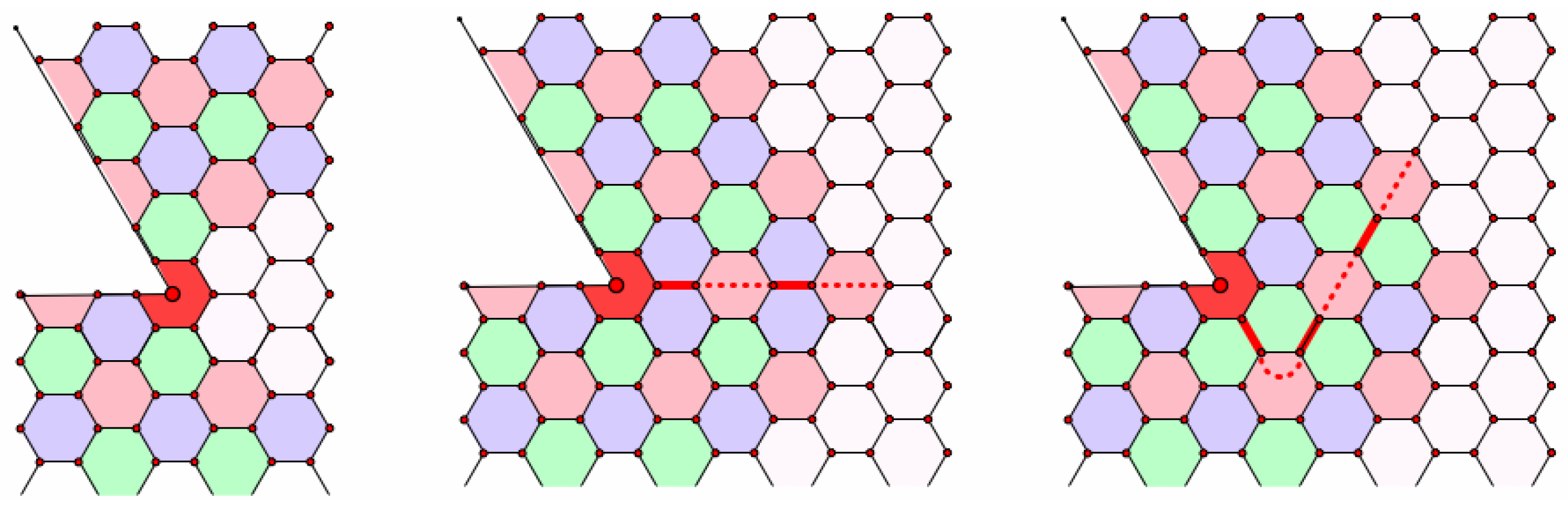
Now, think of starting with a patch of hexagons on a fullerene. Choose an edge-face three-coloring for the patch and think of trying to expand this coloring. As soon as the expansion reaches a pentagon, the face coloring cannot wrap around the pentagon without assigning two adjacent faces the same color. We illustrate this in Figure 8. The incompatibility occurs along a chain consisting of an alternating sequence of faces and edges starting with the pentagon. In the figure, the pentagon is assigned the color red, as are the edges and other faces of the chain; the face color incompatibilities all occur at the edges of the chain. Depending on which direction the chain leaves the pentagon, the incompatibilities are blue or green. As we have illustrated in the figure, the chain can zig-zag. As long as the turns are sharp, the color of incompatibility remains the same; we will restrict our attention to chains with just one color of incompatibility. As we continue to extend the face three coloring, the chain continues to extend and can only terminate in another pentagon. Expanding as far as possible results in an improper face three-coloring where the incompatibilities all occur along six disjoint chains that pair the pentagons. In particular, we have a proper edge-face three-coloring away from these chains.

Figure 8. Building a chain from a pentagon.

Figure 8. Building a chain from a pentagon.

Chains were first introduced in [5]. Formally, the chains that we consider consist of sequences of faces and edges $f_0,e_1,f_1,e_2,\cdots ,e_n,f_n$ where:

• for all i, $e_i$ has exactly one endpoint in $f_{i-1}$, while the other endpoint is in $f_i$;
• if $f_i$ is a hexagon, the endpoints of $e_i$ and $e_{i+1}$ are either opposite or adjacent around the boundary of $f_i$;
• either $f_n=f_0$ and all faces are distinct hexagons or $f_0$ and $f_n$ are distinct pentagons, and all other faces on the chain are distinct hexagons.

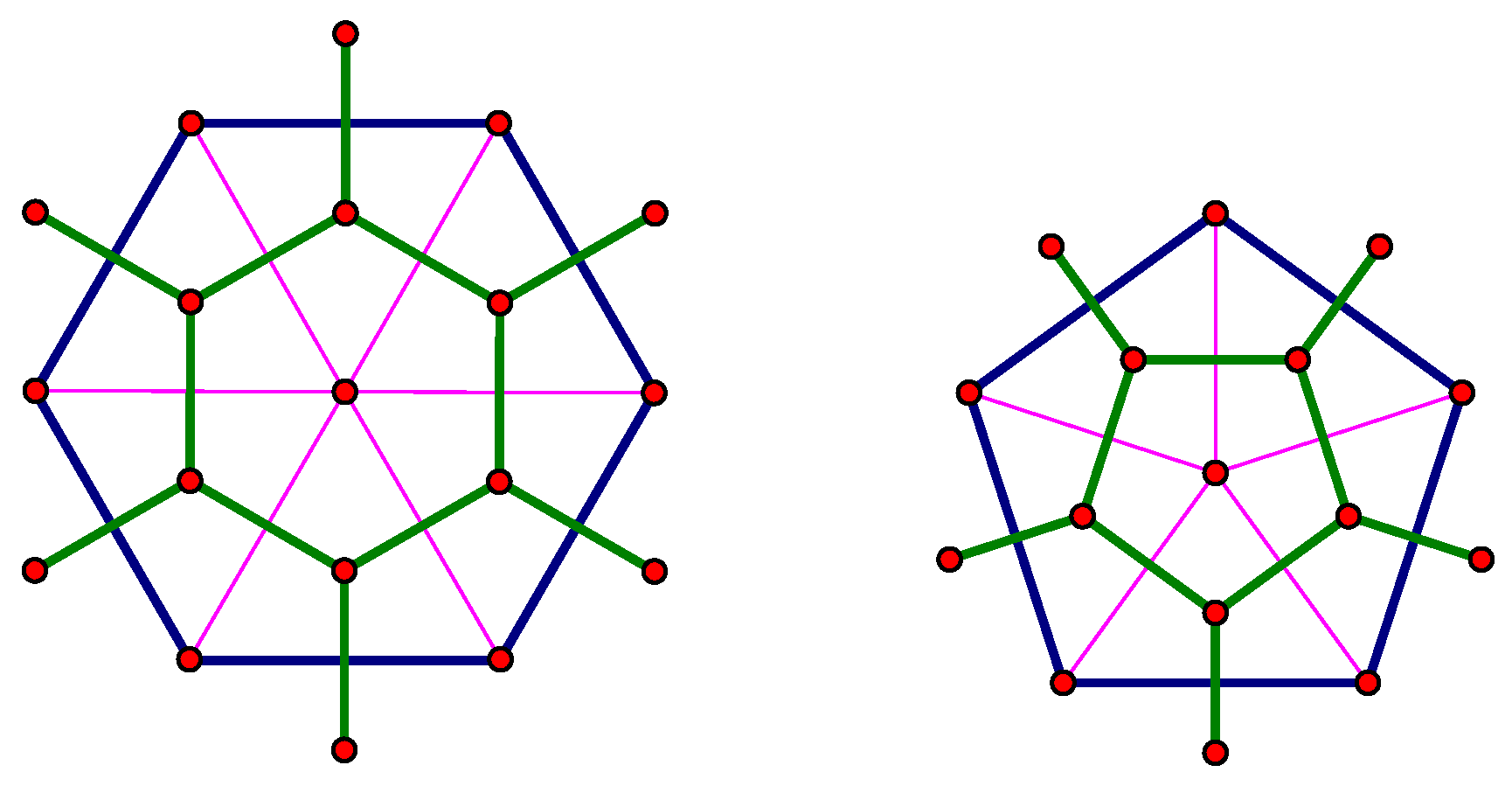
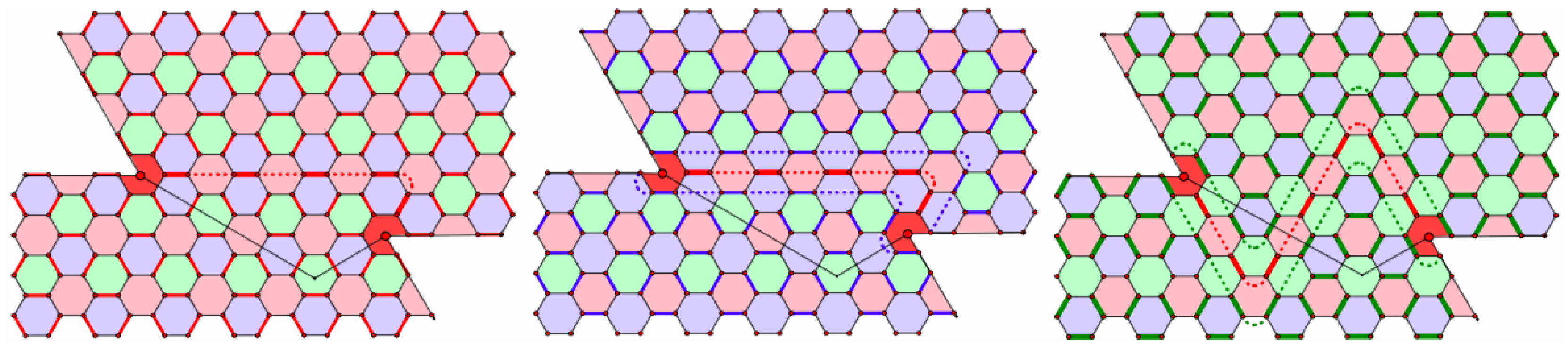
The basic properties of chains have been worked out in [2] and we summarize these basic properties here. Assume that two neighboring pentagons can be joined by a chain. To start with, we restrict our attention to chains that do not swing out around a third pentagon. By a flip we mean interchanging a single left (right) turn by a left-right-left (right-left-right) sequence of turns: the right chain in Figure 9 is obtained from the center chain by flipping face f into face $f^{\prime }$ and flipping face g into face $g^{\prime }$. Two chains are equivalent if one can be transformed into the other by a sequence of such flips. By the length of a chain, we mean the number of edges in the chain. We note that a flip does not change the length of a chain, and it does not change the color of incompatibility. A chain that has two consecutive right turns can be shortened by directly connecting the face just before the first right turn and the face directly after the second right turn; see Figure 10. We restrict our attention to chains that cannot be shortened, and they fall into just two equivalence classes: those with blue incompatibility and those with green incompatibility.

Considering Figure 9, we note that the Coxeter coordinates of the segment joining these two pentagons are $(5,2)$ and that five is congruent to two mod three. In fact, two neighboring pentagons with Coxeter coordinates $(p,q)$ where p and q are not congruent mod three can only be joined by chains that wrap around a third pentagon. In this example, the chain with the blue incompatibility has length five, while the two equivalent chains with the green incompatibility have length seven. When two neighboring pentagons have Coxeter coordinates $(p,q)$ where p and q are congruent mod three, then the minimal chains joining them fall into two equivalence classes where:

• the chains in one equivalence class have length $max\{p,q\}$ and a color of incompatibility different from the color of the faces of the chain;
• the chains in the other equivalence class have length $p+q$ and the third color as the color of incompatibility.

Figure 9. The properties of simple chains.

Figure 9. The properties of simple chains.

Figure 10. Shortening a chain with two consecutive right turns.

Figure 10. Shortening a chain with two consecutive right turns.

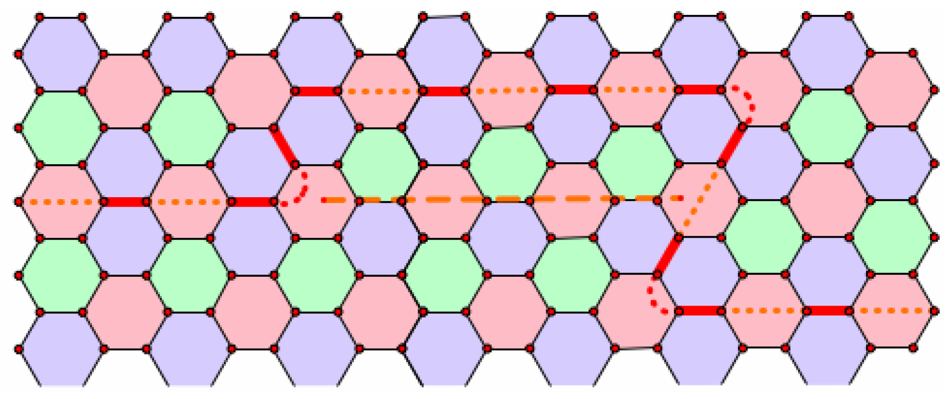
Now, consider choosing the Kekulé structure to be one of the edge color classes away from the chain and try to extend it to include the region around the chain. If we choose the red edges, the same color as the chain, there is a perfect match. See the left-most region in Figure 11. In this case, there is no contribution to the Fries deficit; all blue and green faces are benzene rings, while all red faces are void. Therefore, every red edge belongs to two benzene rings and $|A_0|=|A_1|=0$ in this region. If we choose the blue edges for the Kekulé structure (the color of incompatibility) away from this chain, the red edges of the chain will then complete the Kekulé structure through this region. In this case, the five edges on the chain contribute five to $|A_0|$, while the 12 edges of the closed blue chain surrounding the red chain contribute 12 to $|A_1|$, for a total contribution to the Fries deficit of 22; see the central picture in Figure 11. Finally, if we start with the green edges for the Kekulé structure and extend toward the chain with blue incompatibility, the edges of both the red and blue chains will be incorporated into the Kekulé structure. The edges of the red and blue chains will now contribute 17 to $|A_0|$, and there will be a closed green chain surrounding the blue chain contributing 16 to $|A_1|$. This gives a contribution of 50 to the Fries deficit. However, we can do much better if we use the slightly longer red chain with green as the color of incompatibility, the right-hand region. In this case, the red chain contributes seven to $|A_0|$, while the edges of the closed green chain surrounding the red chain contribute 16 to $|A_1|$, for a total contribution to the Fries deficit of just 30.

Figure 11. Contribution of simple chains to the Fries deficit.

Figure 11. Contribution of simple chains to the Fries deficit.

If we choose the green faces in Figure 11 to be the Clar faces with either the red or blue Kekulé structure, A consists of the five edges of the red chain. If we choose the red faces for C, A will consist of either the 17 edges of the red and blue chains from the center picture or the 23 edges of the red and green chains from the right-hand picture. Finally, if we choose the blue faces to be the Clar faces with the green Kekulé structure, A consists of the seven edges of the red chain. If we were to choose the blue faces to be the Clar faces with the red Kekulé structure, we could only include the blue faces from one side of the red chain, say the top and right-most blue faces bordering the red chain. In this case, the set A would consist of the seven red edges on the bottom four blue faces, but not on the chain. However, this is just the edges of the right-most chain folded.

Now, to compute the Fries or Clar number of a fullerene, we consider all possible sets of pairing chains. Then, for each choice of pairing chains, we consider each of the three edge color classes, extend to the chains and compute the Clar and Fries deficits. In both cases, the number of choices is finite; nevertheless, one may need to consider many different possibilities. We now wish to illustrate that if we carry out this investigation for the three smallest fullerenes in a similarity class, we can then deduce the Clar and Fries numbers for every member of that class.

First consider leapfrog fullerenes. Since in a leapfrog fullerene, the Coxeter coordinates of any segment joining two pentagons are congruent modulo three, all pentagons are assigned the same color, and taking that color class of edges gives $\frac{1}{3}\left|V\right|$ for the Fries number. We still must find a chain decomposition to compute the Clar number, but that is usually straight forward. Therefore, we concentrate on the more complicated problems with the non-leapfrog similarity classes.

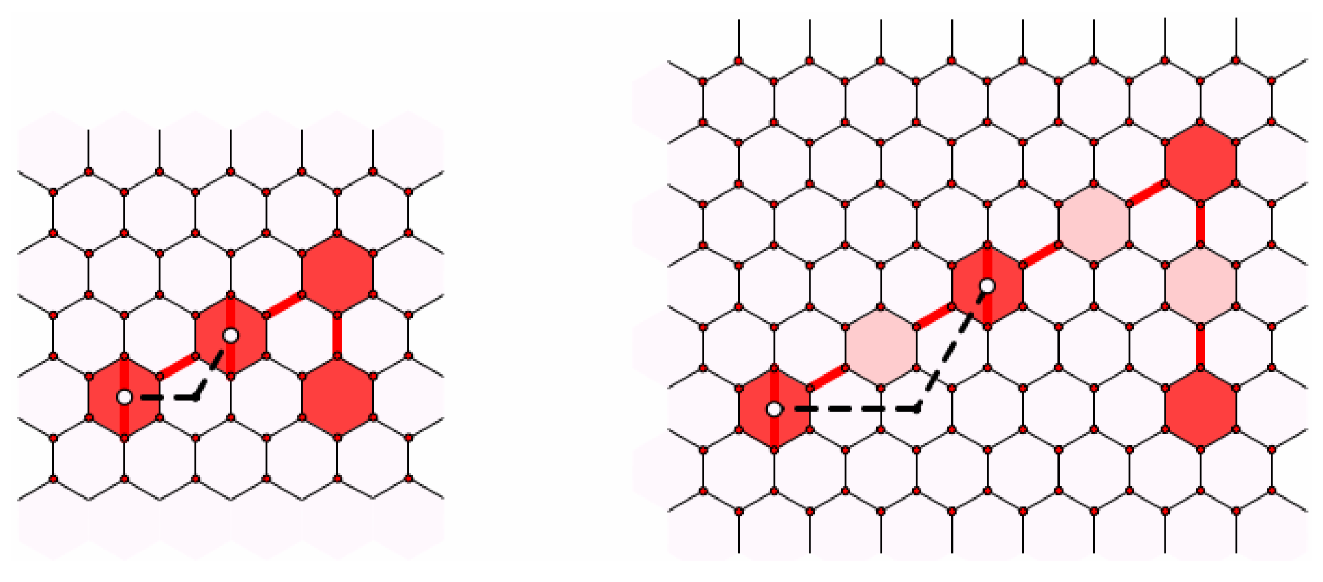
Our first task is to consider the effect of similarity on chains. Let Γ be a reduced non-leapfrog fullerene and ${\Gamma }^{\prime }$ be the similar fullerene expanded by the factor m. Suppose that we have a chain joining neighboring pentagons f and g in Γ, and let $f^{\prime }$ and $g^{\prime }$ be the images of f and g under the dilation. Consider the image of the faces of the chain under the expansion. In Figure 12, we consider part of such a chain where $m=2$. The Coxeter coordinates for the segment joining consecutive faces on the chain in Γ are $(1,1)$; hence, the Coxeter coordinates for the segment joining images of these faces in ${\Gamma }^{\prime }$ are $(m,m)$ ($(2,2)$ in the figure). Hence, the $m-1$ faces along the segment joining image faces may be added in to complete a chain joining $f^{\prime }$ to $g^{\prime }$. Therefore, any chain in the reduced fullerene may be lifted to any similar fullerene. We should note here that when a chain wraps around another pentagon, it will take two consecutive right (or left) turns. However, it cannot be shortened because the shortening path would cut off or through the pentagon it is wrapping around; see Figure 10. Now, when we lift a chain that is wrapped around a pentagon, the lifted image may pull far enough away from the pentagon that it can be shortened (pulled tighter around the pentagon). When we say that a chain is lifted, we will assume that it has also been shortened as much as is possible.

Figure 12. Dilating a chain.

Figure 12. Dilating a chain.

Now, suppose that pentagons f and g in the reduced fullerene Γ are sent to pentagons $f^{\prime }$ and $g^{\prime }$ in a similar fullerene ${\Gamma }_m$. As we just showed, chains joining f and g lift to chains joining $f^{\prime }$ and $g^{\prime }$. However, of course, not all chains joining $f^{\prime }$ and $g^{\prime }$ are one of these dilated chains. If f and g are neighbors in Γ, then $f^{\prime }$ and $g^{\prime }$ are neighbors in ${\Gamma }_m$. Furthermore, the shortest chains in both cases fall into just two equivalence classes under the flipping operation identified by the color of incompatibility. Lifting one chain of each class joining f and g in Γ gives one representative for each class joining $f^{\prime }$ and $g^{\prime }$ in ${\Gamma }_m$. It is also true for chains that join f and g by wrapping around one or more pentagons: there will be just two equivalence classes of shortest paths that wrap around the same pentagons in the same order. The only question that remains is: could there be a pair of pentagons in ${\Gamma }_m$ that can be joined by a chain in ${\Gamma }_m$ where the corresponding pair in Γ cannot be joined by a chain in Γ? The answer is yes when the scaling factor is a multiple of three and no otherwise.

When the scaling factor m is three, all segments joining neighboring pentagons have Coxeter coordinates congruent modulo three; so, ${\Gamma }_m$ is a leapfrog fullerene, and as we have already observed, any pair of pentagons may be joined by a chain including pairs that cannot be paired in the reduced fullerene. 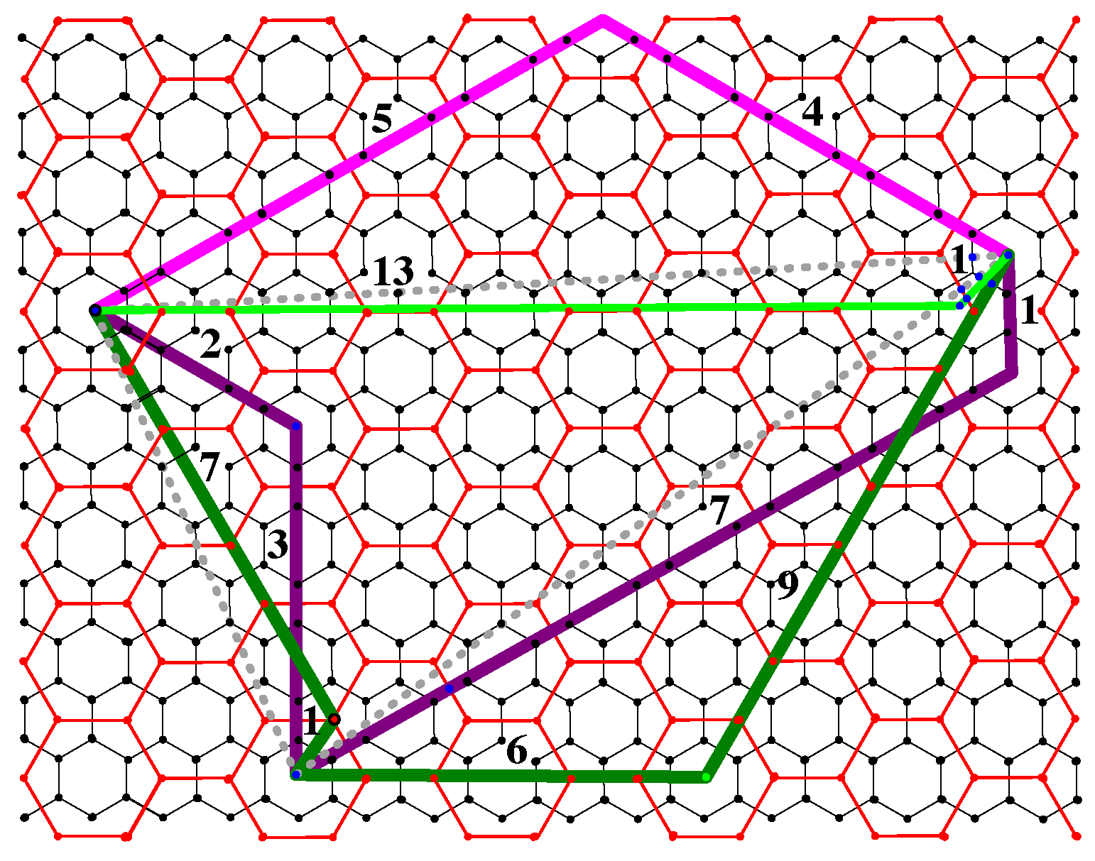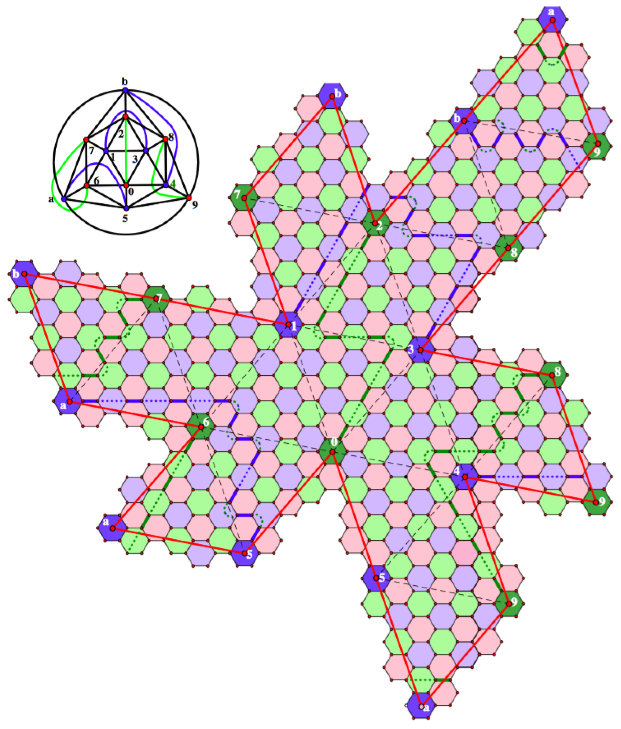However, when the scaling factor m is not a multiple of three, then all pairing chains in ${\Gamma }_m$ are equivalent to a chain lifted from Γ. In view of this fact, we find the best chain decomposition for the reduced fullerene and lift it to the non-leapfrog fullerenes in the similarity class. To illustrate this process, we consider the best chain decomposition for the reduce icosahedral fullerene with coordinates $(2,1)$; this is pictured in Figure 13. Here, we use some chains that wrap around a pentagon. For example, Pentagons 1 and 3 cannot be joined by a direct chain, but they can be joined by a chain that wraps around Pentagon 2. The feature that makes this pairing so good is that we have three green chains where blue is the color of incompatibility and three blue chains with green the color of incompatibility. Choosing the green edges for the Kekulé structure, the green chains contribute nothing to the Fries deficit, while the blue chain has the smallest possible contribution (as described in the paragraph after Figure 11). If choosing the red faces for the Char set, then only the lengths of the chains contribute to the Clar deficit, the least possible for a chain decomposition.

In Figure 14, we have scaled up this chain decomposition by a factor of two.

Figure 13. The best chain decomposition for the reduce icosahedral fullerene with coordinates $(2,1)$.

Figure 13. The best chain decomposition for the reduce icosahedral fullerene with coordinates $(2,1)$.

Figure 14. The scaled up chain decomposition for the similar icosahedral fullerene with coordinates $(4,2)$.

Figure 14. The scaled up chain decomposition for the similar icosahedral fullerene with coordinates $(4,2)$.

Here, we again have three green and three blue chains; however, the color of incompatibility for all chains is red. Therefore, the contributions to the Fries and Clar deficits are not simply scaled up; the contributions to the deficits are quite large. We could get back to blue and green as the incompatibility colors by switching in each case to a chain in the other equivalence class. For example, the length eight green chain joining Pentagons 0 and 2 with red incompatibility could be replaced by a length 10 green chain joining Pentagons 0 and 2 with blue incompatibility. However, this would increase the contributions to deficits. It is natural to ask if we must reconsider every other non-leapfrog fullerene in the similarity class. The answer is no. If we expand by a factor of four, in fact by any factor congruent to one modulo three, our basic chain decomposition will scale up to three green chains with blue the color of incompatibility and three blue chains with green the color of incompatibility and lengths increased by a factor of four. If we expand by a factor of five, in fact by any factor congruent to two modulo three, our basic chain decomposition will scale up to three green chains and three blue chains with all incompatibilities colored red. Hence, once we find the best chain decomposition for the expansion by two cases, we can use that decomposition for all of the expansions by a factor congruent to two mod three.

Therefore, for each non-leapfrog similarity class, we need only find the best chain decomposition for the Clar number and the best chain decomposition for the Fries number in each of the three smallest members of the class. Additionally, from these chain decompositions, we can derive formulas for the Clar and Fries numbers for all members of the similarity class.