2. Jacobi Last Multiplier and Its Properties
In this section, we recall the definition and properties of the Jacobi last multiplier, its connection to Lie symmetries and to Lagrangians (namely, calculus of variations).
The method of the Jacobi last multiplier [
10,
11] (an English translation of [
11] is available in [
12]) provides a means to determine all of the solutions of the partial differential equation:
or its equivalent associated Lagrange’s system:
In fact, if one knows the Jacobi last multiplier and all, but one of the solutions, namely
solutions, then the last solution can be obtained by a quadrature. The Jacobi last multiplier
M is given by:
where
and
are
solutions of (3) or, equivalently, first integrals of (4) independent of each other. This means that
M is a function of the variables
and depends on the chosen
solutions, in the sense that it varies as they vary. The essential properties of the Jacobi last multiplier are:
- (a)
If one selects a different set of
independent solutions
of Equation (
3), then the corresponding last multiplier
N is linked to
M by the relationship:
- (b)
Given a non-singular transformation of variables:
then the last multiplier
of
is given by:
where
M obviously comes from the
solutions of
, which correspond to those chosen for
through the inverse transformation
.
- (c)
One can prove that each multiplier
M is a solution of the following linear partial differential equation:
and
vice versa, every solution
M of this equation is a Jacobi last multiplier.
- (d)
If one knows two Jacobi last multipliers
and
of Equation (
3), then their ratio is a solution ω of (3) or, equivalently, a first integral of (4). Naturally, the ratio may be quite trivial, namely a constant;
vice versa, the product of a multiplier
times any solution ω yields another last multiplier
.
Since the existence of a solution/first integral is consequent upon the existence of symmetry, an alternative formulation in terms of symmetries was provided by Lie [
13,
14]. A clear treatment of the formulation in terms of solutions/first integrals and symmetries is given by Bianchi [
15]. If we know
symmetries of (3)/4), say:
a Jacobi last multiplier is given by
, provided that
, where:
There is an obvious corollary to the results of the Jacobi mentioned above. In the case that there exists a constant multiplier, the determinant is a first integral. This result is potentially very useful in the search for first integrals of systems of ordinary differential equations. In particular, if each component of the vector field of the equation of motion is missing, the variable associated with that component, i.e., , the last multiplier is a constant, and any other Jacobi last multiplier is a first integral.
Another property of the Jacobi last multiplier is its (almost forgotten) relationship with the Lagrangian,
, for any second-order equation:
namely [
11,
16]:
where
satisfies the following equation:
Then, Equation (
10) becomes the Euler–Lagrange equation:
The proof is given by taking the derivative of (13) by
and showing that this yields (12). If one knows a Jacobi last multiplier, then
L can be obtained by a double integration,
i.e.:
where
and
are functions of
t and
x, which have to satisfy a single partial differential equation related to (10) [
17]. As was shown in [
17],
are related to the gauge function
. In fact, we may assume:
where
has to satisfy the mentioned partial differential equation and
F is obviously arbitrary.
In [
18], it was shown that a system of two first-order ordinary differential equations:
always admits a linear Lagrangian of the form:
The key is a function
W, such that:
and
It is obvious that Equation (
19) is Equation (
7) of the Jacobi last multiplier for system (16), as it was point out in [
8]. Therefore, once a Jacobi last multiplier
has been found, then a Lagrangian of system (16) can be obtained by two integrations,
i.e.,
where
satisfies two linear differential equations of first order that can be always integrated and
is the arbitrary gauge function that should be taken into consideration in order to apply correctly Noether’s theorem [
9]. If a Noether symmetry:
exists for the Lagrangian
L in (20), then a first integral of system (16) is:
We underline that and always disappear from the expression of the first integral (22) thanks to the linearity of the Lagrangian (20) and formula (20).
3. Lie Symmetries of System (1)–(2)
It is well known to practitioners of Lie group analysis that a first-order system of ordinary differential equations admits an infinite-dimensional Lie symmetry algebra; e.g., see [
19]. Lie’s theory allows us to integrate system (1)–(2) by quadrature, if we find at least a two-dimensional Lie algebra. In order to find it, we derive
from (2),
i.e.,
Consequently we obtain a second-order ordinary differential equation (ODE) in
,
and search for its Lie symmetry algebra. An operator Γ:
is said to generate a Lie point symmetry group of an equation of second-order, e.g.,
if its second prolongation:
applied to (26), on its solutions, is identically equal to zero,
i.e.:
A trivial Lie point symmetry of system (1)–(2) and also of Equation (
24) is translation in time,
i.e.,
Using
ad hoc REDUCE interactive programs [
20], we find that Equation (
24) admits at least another symmetry in two cases. Of course, any of those symmetries corresponds to a symmetry of system (1)–(2), as we show below.
Case (A)
If the following relationship among the parameters
and
c is satisfied (condition
does not yield a second Lie symmetry of Equation (
24)):
then Equation (
24) admits a two-dimensional Lie symmetry algebra generated by (if
, then (29) implies that
; this is a particular example of Case (A), and we discuss it in Remark 3 of
Section 4):
This Lie symmetry algebra is non-Abelian and transitive,
i.e., of Type III in Lie’s classification of two-dimensional algebras in the real plane [
14] (this classification can also be found in Bianchi’s book [
15] and in modern textbooks, e.g., [
21]). Therefore, to integrate Equation (
24), we have to transform it into its canonical form, as given by Lie himself,
i.e.,
where
are the new independent and dependent variables, respectively,
is an arbitrary function of
and the two-dimensional canonical Lie algebra of Type III is generated by the following operators:
We determine:
and consequently, (24) becomes:
which can be integrated by two quadratures to yield:
with
two arbitrary constants.
Case (B)
If the following relationship among the parameters
a and
c is satisfied:
then Equation (
24) admits a two-dimensional Lie symmetry algebra generated by:
This Lie symmetry algebra is also non-Abelian and transitive. Therefore, we can derive the corresponding canonical transformation,
i.e.,
and consequently, (24) becomes:
which can be integrated by two quadratures to yield:
with
two arbitrary constants.
Subcase (B.1)
If in addition to the condition (36), the following relationship among the parameters
h and
c is satisfied:
then Equation (
24),
i.e.,
admits a three-dimensional Lie symmetry algebra generated by:
This algebra is a representation of
. It was shown in [
22] that if we treat (42) as a first integral, namely if we solve the equation with respect to
(this choice, instead of
K, is just for convenience),
i.e.:
then a linearizable third-order equation is obtained,
i.e.,
In fact, this equation admits a seven-dimensional Lie symmetry algebra generated by the following operators:
We remark that we could not solve Equation (
42) with respect to
c since it is not an essential constant: in fact, we could have eliminated it from system (1)–(2) by rescaling. Indeed, the third-order equation that one gets through
c, namely:
admits a two-dimensional Lie symmetry algebra, generated by
, and consequently, it is not linearizable.
Following Lie [
14], the linearizing transformation of Equation (
45) is given by finding a two-dimensional Abelian intransitive subalgebra and putting it into the canonical form
. Since a two-dimensional Abelian intransitive subalgebra is that generated by
and
, then the point transformation:
takes (45) into the following linear equation:
Its general solution simply is:
with
arbitrary constants, that, replaced into (45), yields the general solution:
Since the original Equation (
42) is of second order, then one of the constants of integrations
should be superfluous. Indeed, if we replace (50) into (44), then the following condition is obtained:
that yields:
Finally, the general solution of Equation (
42) is:
and consequently, by means of (23), the general solution of system (1)–(2),
i.e.,
is given by:
Since
, this solution corresponds to asymptotic death for all [
7]. We present two particular instances of the general solution (56) in
Figure 1 and
Figure 2.
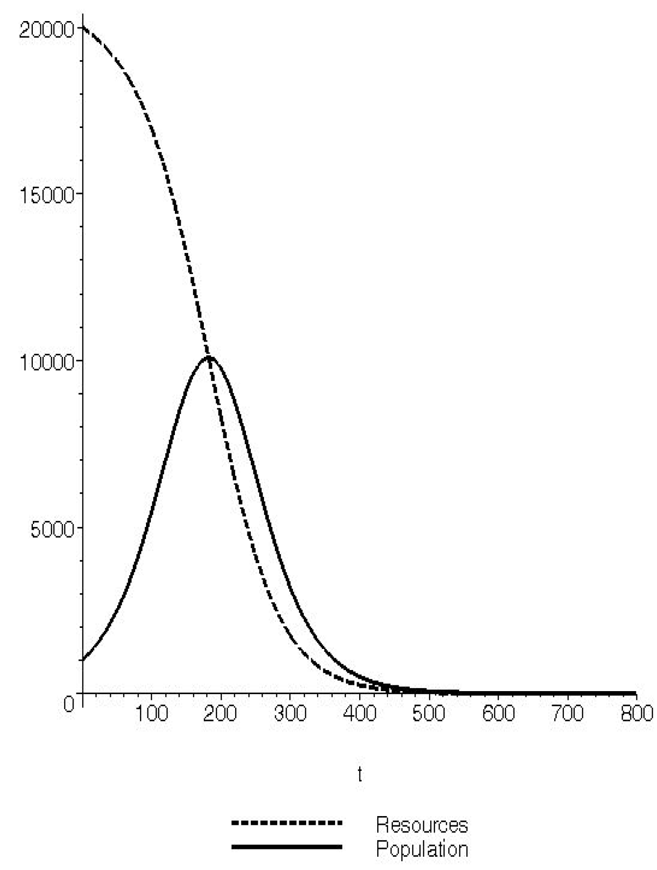
Figure 1.
The amount of resources and that of the population for the values of the parameters , and for the initial conditions 1000, 20000.
Figure 1.
The amount of resources and that of the population for the values of the parameters , and for the initial conditions 1000, 20000.
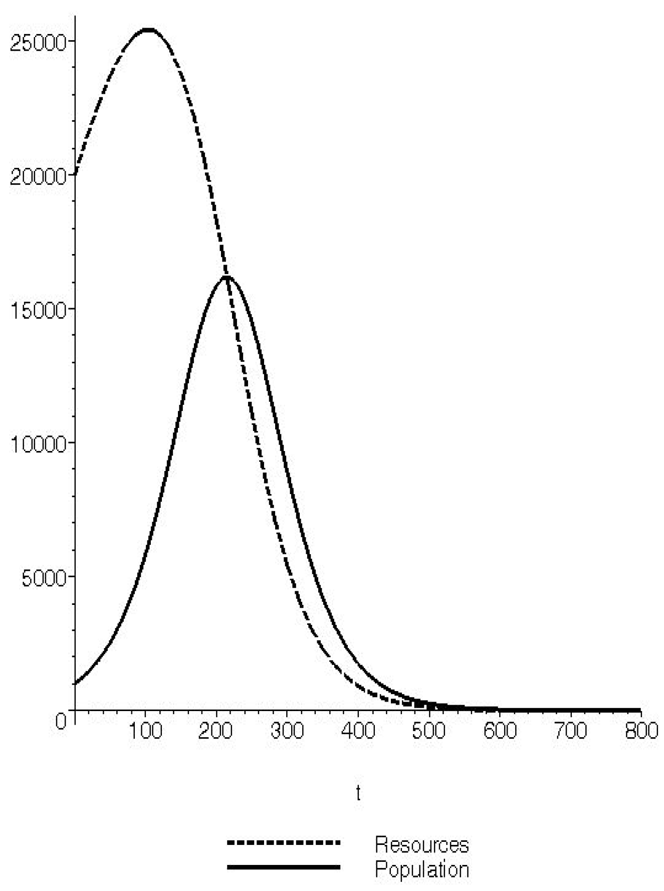
Figure 2.
The amount of resources and that of the population for the values of the parameters , and for the initial conditions 1000, 20000.
Figure 2.
The amount of resources and that of the population for the values of the parameters , and for the initial conditions 1000, 20000.
It is interesting to remark that if we double the carrying capacity
K leaving the other parameters and initial conditions unaltered, the amount of resources
actually grows along with the population
at least for a period of time (approximately a century in
Figure 2) before decreasing dramatically.
4. Jacobi Last Multipliers, Lagrangians and First Integrals of System (1)–(2)
A Jacobi last multiplier for system (1)–(2) has to satisfy Equation (
7),
i.e.,
As in [
8], we assume that
has the following form:
where
are constants to be determined. Replacing this
into system (1)–(2) yields:
Therefore, the following Lagrangian of system (1) and (2) is obtained by means of Equation (
20):
It is obvious that if
, then the Lagrangian
does not exist. Indeed, if:
then the Jacobi Last Multiplier (59) becomes:
and consequently, the Lagrangian of system (1)–(2) is:
The Jacobi Last Multiplier (59) yields the following Jacobi last multiplier of Equation (
24) by means of the application of Property (b):
and consequently, the following Lagrangian is derived by means of (14):
If the following condition on the parameters is satisfied,
i.e.,
then the trivial Lie symmetry (28) admitted by system (1)–(2) and Equation (
24) is also a Noether symmetry (Equation (
24) does not admit another Lie symmetry). Consequently, Noether’s theorem [
9] yields the following first integral:
of Equation (
24),
i.e.,
Replacing
u with
and
with
, namely the RHS of Equation (2), into
yields the following first integral of system (1)–(2):
Remark 1: It was shown in [
7], Proposition 6, that if
, then the first integral (69) yields periodic orbits. In particular, if
, it is easy to show that the general solution depends on elliptic functions. ⧫
It is obvious that if either
or
, then the Lagrangian
in (65) does not exist. In fact, if:
then from
in (64),
i.e.,
the following Lagrangian is obtained by means of (14),
i.e.,
This Lagrangian does not admit any Noether point symmetry unless
, and consequently, the Lagrangian (72) admits the Lie symmetry
as Noether symmetry and the following first integral is derived:
the gauge function being
.
Replacing
u with
and
with
, namely the RHS of Equation (2), into
yields the following first integral of system (1)–(2):
Remark 2: The case
is a particular example of Case (B), and consequently, Equation (
24),
i.e.,
admits the two Lie symmetries (37),
i.e.,
Another Jacobi last multiplier can be obtained from the reciprocal of (9),
i.e.,
Surprisingly, we do not obtain another Jacobi last multiplier. Indeed, is equal to in (71), apart from an unessential multiplicative constant. ⧫
If
then from
in (64),
i.e.,
the following Lagrangian is obtained by means of (14),
i.e.,
This Lagrangian does not admit any Noether point symmetry unless either of the following further conditions are also satisfied,
i.e.,
or
If
, then the Lagrangian (80) admits the trivial Lie symmetry (28) as Noether symmetry, and consequently, the following first integral is derived:
Replacing
u with
and
with
, namely the RHS of Equation (2), into
yields the following first integral of system (1)–(2):
Remark 3: The case
is a particular example of Case (A), and consequently, Equation (
24),
i.e.,
admits the two Lie symmetries (30),
i.e.,
Its general solution can be determined through the canonical variables, as explained in the previous section, although in implicit form,
i.e.,
Another Jacobi last multiplier (hence, another Lagrangian) for Equation (
85) can be obtained from the reciprocal of (9),
i.e.,
Because of Property (d), the ratio of the Jacobi last multiplier in (79),
i.e.,
, with that found in Equation (
88),
i.e.,
, yields a first integral that surprisingly is just
, apart from an unessential multiplicative constant. ⧫
If
, then the Lagrangian (80) admits the Lie symmetry
as Noether symmetry, and the following first integral is derived:
the gauge function being
.
Replacing
u with
and
with
, namely the RHS of Equation (2), into
yields the following first integral of system (1)–(2):
Remark 4: The case
is another instance of Case (B), and consequently, Equation (
24),
i.e.,
admits the two Lie symmetries (37),
i.e.,
and its general solution can be determined through the canonical variables, as explained in the previous section. Thus, the general solution of system (1)–(2) is that both
and
can go to infinity at the same finite time,
i.e., if:
Another Jacobi last multiplier for Equation (
91) can be obtained from the reciprocal of Equation (
9),
i.e.,
Because of Property (d), the ratio of the Jacobi last multiplier in (79), i.e., , with that found in (95), i.e., , yields a first integral that is just , apart from an unessential multiplicative constant. ⧫
Case (A)
If condition (29) is satisfied, then the Lagrangian (65) admits the Lie symmetry
in (30) as Noether symmetry, with gauge function
and consequently, Noether’s theorem [
9] yields the following first integral:
of Equation (
24),
i.e.,
Replacing
u with
and
with
, namely the RHS of Equation (2), into
yields the following first integral of system (1)–(2):
Another Jacobi last multiplier, and consequently Lagrangian, can be obtained by means of the two Lie symmetries (30) through (9),
i.e.,
The corresponding Lagrangian admits one Lie symmetry as Noether symmetry, with gauge function
,
i.e.,
in (30), and consequently, the following first integral:
We remark that the two first integrals and are not functionally independent.
Case (B)
If condition (36) is satisfied, then the Lagrangian (65) admits the Lie symmetry
in (37) as Noether symmetry, with gauge function
, and consequently, Noether’s theorem [
9] yields the following first integral (
):
of Equation (
24),
i.e.,
Replacing
u with
and
with
, namely the RHS of Equation (2), into
yields the following first integral of system (1)–(2):
Another Jacobi last multiplier, and consequently Lagrangian, can be obtained by means of the two Lie symmetries (37) through (9),
i.e.,
The corresponding Lagrangian admits only the Lie symmetry
in (37) as Noether symmetry, with gauge function
, and consequently, the following first integral:
We remark that the two first integrals and are not functionally independent.
Subcase (B.1)
If condition (41) is satisfied, then the Lagrangian (65) admits all three Lie symmetries in (43) as Noether symmetries, with gauge functions
, and consequently, Noether’s theorem [
9] yields the following three first integrals:
of Equation (
24),
i.e.,
Three more Jacobi last multipliers, and consequently, three Lagrangians, can be obtained by means of the three Lie symmetries (43) through (9),
i.e.,
Since the ratio of two Jacobi last multipliers is a first integral, then we can obtain three first integrals of Equation (
107),
i.e.,
The Lagrangian corresponding to
admits only the Lie symmetry
in (43) as Noether symmetry, with gauge function
, and consequently, Noether’s theorem [
9] yields the following first integral:
The Lagrangian corresponding to
admits only the Lie symmetry
in (43) as Noether symmetry, with gauge function
, and consequently, Noether’s theorem [
9] yields the following first integral:
The Lagrangian corresponding to
admits only the Lie symmetry
in (43) as Noether symmetry, and consequently, Noether’s theorem [
9] yields the following first integral:
Of course, of all these nine first integrals, only two are functionally independent.
5. Discussion and Final Remarks
In this paper, we have determined different cases that fit the qualitative prediction (in [
7], it was assumed
) given in [
7]. Assuming
, then the solution (56) with
corresponds (since
and
) to Proposition 2, namely the case of asymptotic death for all, with both the population and the resources going to zero at infinity. Furthermore, the ratio of population over resources goes asymptotically to 2,
i.e.,
, as predicted in [
7]. Indeed, solution (56) shows that resources decrease, while the population grows exponentially
for an extended period of time followed by a
catastrophic elimination [
7], as can also be seen in
Figure 1. However, for at least a period of time, resources may increase along with the population, as shown in
Figure 2, if the carrying capacity
K is large enough.
In [
7], one first integral was derived under the condition
(Proposition 6). It corresponds to our first integral
I in (69) under the condition
. We have derived many other first integrals and also the general solution of system (1)–(2) in closed form, as well as the general solution of Equation (
24) in implicit form:
the first integral in (74) if ;
the first integral in (84) and also the general solution (87) if ;
the first integral in (90) and also the general solution (94) if ;
the first integral in (98) if , that corresponds to Proposition 3 (, );
the first integral in (103) if , that corresponds to Proposition 1 ().
Last, but not least, we were able to find a Lagrangian (60) for system (1)–(2) and any value of the involved parameters (if the Lagrangian is (63)).
Recently, archeological findings have pointed out that Polynesian rats may have greatly contributed to the tree destruction on Easter Island [
23]. Consequently, in [
24], rats have been included in the mathematical model, leading to three nonlinear first-order differential equations. The chaotic nature of that system has subsequently been determined in [
25]. Can symmetries help since they have always been associated with non-chaotic systems? We recall that in [
26], Lie symmetries yielded an exact transformation that turned a butterfly into a tornado (and
vice versa), and the chaotic features of the Lorenz system [
27] were thus tamed. Could the chaotic features of the rats-trees-islanders model be equally tamed? We hope to address this question in the near future.


