Symmetries Shared by the Poincaré Group and the Poincaré Sphere

1
Center for Fundamental Physics, University of Maryland, College Park, MD 20742, USA
2
Department of Radiology, New York University, New York, NY 10016, USA
*
Author to whom correspondence should be addressed.
Symmetry 2013, 5(3), 233-252; https://doi.org/10.3390/sym5030233
Submission received: 29 May 2013
/
Revised: 9 June 2013
/
Accepted: 9 June 2013
/
Published: 27 June 2013
Abstract
:Henri Poincaré formulated the mathematics of Lorentz transformations, known as the Poincaré group. He also formulated the Poincaré sphere for polarization optics. It is shown that these two mathematical instruments can be derived from the two-by-two representations of the Lorentz group. Wigner’s little groups for internal space-time symmetries are studied in detail. While the particle mass is a Lorentz-invariant quantity, it is shown to be possible to address its variations in terms of the decoherence mechanism in polarization optics.
Keywords:
Poincaré group; Poincaré sphere; Wigner’s little groups; particle mass; decoherence mechanism; two-by-two representations; Lorentz groupClassification:
PACS 03.65.Fd; 03.67.-; 05.30.-d1. Introduction
It was Henri Poincaré who worked out the mathematics of Lorentz transformations before Einstein and Minkowski, and the Poincaré group is the underlying language for special relativity. In order to analyze the polarization of light, Poincaré also constructed a graphic illustration known as the Poincaré sphere [1,2,3].
It is of interest to see whether the Poincaré sphere can also speak the language of special relativity. In that case, we can study the physics of relativity in terms of what we observe in optical laboratories. For that purpose, we note first that the Lorentz group starts as a group of four-by-four matrices, while the Poincaré sphere is based on the two-by-two matrix consisting of four Stokes parameters. Thus, it is essential to find a two-by-two representation of the Lorentz group. Fortunately, this representation exists in the literature [4,5], and we shall use it in this paper.
As for the problems in relativity, we shall discuss here Wigner’s little groups dictating the internal space-time symmetries of relativistic particles [6]. In his original paper of 1939 [7], Wigner considered the subgroups of the Lorentz group, whose transformations leave the four-momentum of a given particle invariant. While this problem has been extensively discussed in the literature, we propose here to study it using Naimark’s two-by-two representation of the Lorentz group [4,5].
This two-by-two representation is useful for communicating with the symmetries of the Poincaré sphere based on the four Stokes parameters, which can take the form of two-by-two matrices. We shall prove here that the Poincaré sphere shares the same symmetry property as that of the Lorentz group, particularly in approaching Wigner’s little groups. By doing this, we can study the Lorentz symmetries of elementary particles from what we observe in optical laboratories.
The present paper starts from an unpublished note based on an invited paper presented by one of the authors (YSK) at the Fedorov Memorial Symposium: Spins and Photonic Beams at Interface held in Minsk (2011) [8]. To this, we have added a detailed discussion of how the decoherence mechanism in polarization optics is mathematically equivalent to a massless particle gaining mass to become a massive particle. We are particularly interested in how the variation of mass can be accommodated in the study of internal space-time symmetries.
In Section 2, we define the symmetry problem we propose to study in this paper. We are interested in the subgroups of the Lorentz group, whose transformations leave the four-momentum of a given particle invariant. This is an old problem and has been repeatedly discussed in the literature [6,7,9]. In this paper, we discuss this problem using the two-by-two formulation of the Lorentz group. This two-by-two language is directly applicable to polarization optics and the Poincaré sphere.
While Wigner formulated his little groups for particles in their given Lorentz frames, we give a formalism applicable to all Lorentz frames. In his 1939 paper, Wigner pointed out that his little groups are different for massive, massless and imaginary-particles. In Section 3, we discuss the possibility of deriving the symmetry properties for massive and imaginary-mass particles from that of the massless particle.
In Section 4, we assemble the variables in polarization optics, and define the matrix operators corresponding to transformations applicable to those variables. We write the Stokes parameters in the form of a two-by-two matrix. The Poincaré sphere can be constructed from this two-by-two Stokes matrix. In Section 5, we note that there can be two radii for the Poincaré sphere. Poincaré’s original sphere has one fixed radius, but this radius can change, depending on the degree of coherence. Based on what we studied in Section 3, we can associate this change of the radius to the change in mass of the particle.
2. Poincaré Group and Wigner’s Little Groups
Poincaré formulated the group theory of Lorentz transformations applicable to four-dimensional space consisting of three space coordinates and one time variable. There are six generators for this group consisting of three rotation and three boost generators.
In addition, Poincaré considered translations applicable to those four space-time variables, with four generators. If we add these four generators to the six generators for the homogenous Lorentz group, the result is the inhomogeneous Lorentz group [7] with ten generators. This larger group is called the Poincaré group in the literature.
The four translation generators produce space-time four-vectors consisting of the energy and momentum. Thus, within the framework of the Poincaré group, we can consider the subgroup of the Lorentz group for a fixed value of momentum [7]. This subgroup defines the internal space-time symmetry of the particle. Let us consider a particle at rest. Its momentum consists of its mass as its time-like variable and zero for the three momentum components.
For convenience, we use the four-vector convention, and .
This four-momentum of Equation (1) is invariant under three-dimensional rotations applicable only to the coordinates. The dynamical variable associated with this rotational degree of freedom is called the spin of the particle.
We are then interested in what happens when the particle moves with a non-zero momentum. If it moves along the z direction, the four-momentum takes the value:
which means:
Accordingly, the little group consists of Lorentz-boosted rotation matrices. This aspect of the little group has been discussed in the literature [6,9]. The question then is whether we could carry out the same logic using two-by-two matrices
Of particular interest is what happens when the transformation parameter, η, becomes very large and the four-momentum becomes that of a massless particle. This problem has also been discussed in the literature within the framework of four-dimensional Minkowski space. The η parameter becomes large when the momentum becomes large, but it can also become large when the mass becomes very small. The two-by-two formulation allows us to study these two cases separately, as we will do in Section 3.
If the particle has an imaginary mass, it moves faster than light and is not observable. Yet, particles of this kind play important roles in Feynman diagrams, and their space-time symmetry should also be studied. In his original paper [7], Wigner studied the little group as the subgroup of the Lorentz group whose transformations leave the four-momentum invariant of the form:
Wigner observed that this four-momentum remains invariant under the Lorentz boost along the x or y direction.
If we boost this four-momentum along the z direction, the four-momentum becomes:
with:
The two-by-two formalism also allows us to study this problem.
In Subsection 2.1, we shall present the two-by-two representation of the Lorentz group. In Subsection 2.2, we shall present Wigner’s little groups in this two-by-two representation. While Wigner’s analysis was based on particles in their fixed Lorentz frames, we are interested in what happens when they start moving. We shall deal with this problem in Section 3.
2.1. Two-by-Two Representation of the Lorentz Groups
The Lorentz group starts with a group of four-by-four matrices performing Lorentz transformations on the Minkowskian vector space of leaving the quantity:
invariant. It is possible to perform this transformation using two-by-two representations [4,5]. This mathematical aspect is known as , the universal covering group for the Lorentz group.
In this two-by-two representation, we write the four-vector as a matrix:
Then, its determinant is precisely the quantity given in Equation (7). Thus, the Lorentz transformation on this matrix is a determinant-preserving transformation. Let us consider the transformation matrix as:
with:
The G matrix starts with four complex numbers. Due to the above condition on its determinant, it has six independent parameters. The group of these G matrices is known to be locally isomorphic to the group of four-by-four matrices performing Lorentz transformations on the four-vector . In other words, for each G matrix, there is a corresponding four-by-four Lorentz-transform matrix, as is illustrated in the Appendix.
The matrix, G, is not a unitary matrix, because its Hermitian conjugate is not always its inverse. The group can have a unitary subgroup, called , performing rotations on electron spins. As far as we can see, this G-matrix formalism was first presented by Naimark in 1954 [4]. Thus, we call this formalism the Naimark representation of the Lorentz group. We shall see first that this representation is convenient for studying space-time symmetries of particles. We shall then note that this Naimark representation is the natural language for the Stokes parameters in polarization optics.
With this point in mind, we can now consider the transformation:
Since G is not a unitary matrix, it is not a unitary transformation. In order to tell this difference, we call this the “Naimark transformation”. This expression can be written explicitly as:
For this transformation, we have to deal with four complex numbers. However, for all practical purposes, we may work with two Hermitian matrices:
and two symmetric matrices:
whose Hermitian conjugates are not their inverses. The two Hermitian matrices in Equation (13) lead to rotations around the z and y axes, respectively. The symmetric matrices in Equation (14) perform Lorentz boosts along the z and x directions, respectively.
Repeated applications of these four matrices will lead to the most general form of the G matrix of Equation (9) with six independent parameters. For each two-by-two Naimark transformation, there is a four-by-four matrix performing the corresponding Lorentz transformation on the four-component four-vector. In the Appendix, the four-by-four equivalents are given for the matrices of Equations (13) and (14).
It was Einstein who defined the energy-momentum four-vector and showed that it also has the same Lorentz-transformation law as the space-time four-vector. We write the energy-momentum four-vector as:
with:
which means:
where m is the particle mass.
Now, Einstein’s transformation law can be written as:
or explicitly:
2.2. Wigner’s Little Groups
Later in 1939 [7], Wigner was interested in constructing subgroups of the Lorentz group whose transformations leave a given four-momentum invariant. He called these subsets “little groups”. Thus, Wigner’s little group consists of two-by-two matrices satisfying:
This two-by-two W matrix is not an identity matrix, but tells about the internal space-time symmetry of a particle with a given energy-momentum four-vector. This aspect was not known when Einstein formulated his special relativity in 1905. The internal space-time symmetry was not an issue at that time.
If its determinant is a positive number, the P matrix can be brought to a form proportional to:
corresponding to a massive particle at rest.
If the determinant is negative, it can be brought to a form proportional to:
corresponding to an imaginary-mass particle moving faster than light along the z direction, with its vanishing energy component.
If the determinant is zero, we may write P as:
which is proportional to the four-momentum matrix for a massless particle moving along the z direction.
For all three of the above cases, the matrix of the form:
will satisfy the Wigner condition of Equation (20). This matrix corresponds to rotations around the z axis, as is shown in the Appendix.
For the massive particle with the four-momentum of Equation (21), the Naimark transformations with the rotation matrix of the form:
also leave the P matrix of Equation (21) invariant. Together with the matrix, this rotation matrix leads to the subgroup consisting of the unitary subset of the G matrices. The unitary subset of G is , corresponding to the three-dimensional rotation group dictating the spin of the particle [9].
For the massless case, the transformations with the triangular matrix of the form:
leave the momentum matrix of Equation (23) invariant. The physics of this matrix has a stormy history, and the variable, γ, leads to gauge transformation applicable to massless particles [6,10].
For a particle with its imaginary mass, the W matrix of the form:
will leave the four-momentum of Equation (22) invariant. This unobservable particle does not appear to have observable internal space-time degrees of freedom.
Table 1 summarizes the transformation matrices for Wigner’s subgroups for massive, massless and imaginary-mass particles. Of course, it is a challenging problem to have one expression for all those three cases, and this problem has been addressed in the literature [11].

Table 1.
Wigner’s Little Groups. The little groups are the subgroups of the Lorentz group, whose transformations leave the four-momentum of a given particle invariant. Thus, the little groups define the internal space-time symmetries of particles. The four-momentum remains invariant under the rotation around it. In addition, the four-momentum remains invariant under the following transformations. These transformations are different for massive, massless and imaginary-mass particles.
| Particle mass | Four-momentum | Transform matrices | ||
|---|---|---|---|---|
| Massive | ||||
| Massless | ||||
| Imaginary mass |
3. Lorentz Completion of Wigner’s Little Groups
In his original paper [7], Wigner worked out his little groups for specific Lorentz frames. For the massive particle, he constructed his little group in the frame where the particle is at rest. For the imaginary-mass particle, the energy-component of his frame is zero.
For the massless particle, it moves along the z direction with a nonzero momentum. There are no specific frames particularly convenient for us. Thus, the specific frame can be chosen for an arbitrary value of the momentum, and the triangular matrix of Equation (26) should remain invariant under Lorentz boosts along the z direction.
For the massive particle, let us Lorentz-boost the four-momentum matrix of Equation (21) by performing a Naimark transformation:
which leads to:
This resulting matrix corresponds to the Lorentz-boosted four-momentum given in Equation (2). For simplicity, we let hereafter in this paper. The Lorentz transformation applicable to the four-momentum matrix is not a similarity transformation, but it is a Naimark transformation, as defined in Equation (11).
On the other hand, the rotation matrix of Equation (25) is Lorentz-boosted as a similarity transformation:
and it becomes:
If we perform the Naimark transformation of the four-momentum matrix of Equation (29) with this Lorentz-boosted rotation matrix:
the result is the four-momentum matrix of Equation (29). This means that the Lorentz-boosted rotation matrix of Equation (31) represents the little group, whose transformations leave the four-momentum matrix of Equation (29) invariant.
For the imaginary-mass case, the Lorentz boosted four-momentum matrix becomes:
For the massless case, if we boost the four-momentum matrix of Equation (23), the result is:
Here, the η parameter is an independent variable and cannot be defined in terms of the momentum or energy.
The remaining problem is to see whether the massive and imaginary-mass cases collapse to the massless case in the large η limit. This variable becomes large when the momentum becomes large or the mass becomes small. We shall discuss these two cases separately.
3.1. Large-Momentum Limit
While Wigner defined his little group for the massive particle in its rest frame in his original paper [7], the little group represented by Equation (31) is applicable to the moving particle, whose four-momentum is given in Equation (29). This matrix can also be written as:
In the limit of large η, we can change the above expression into:
This process is continuous, but not necessarily analytic [11]. After making this transition, we can come back to the original frame to obtain the four momentum matrix of Equation (23).
The remaining problem is the Lorentz-boosted rotation matrix of Equation (31). If this matrix is going to remain finite as η approaches infinity, the upper-right element should be finite for large values of η. Let it be γ. Then:
This means that angle θ has to become zero. As a consequence, the little group matrix of Equation (31) becomes the triangular matrix given in Equation (26) for massless particles.
Imaginary-mass particles move faster than light, and they are not observable. On the other hand, the mathematics applicable to Wigner’s little group for this particle has been useful in the two-by-two beam transfer matrix in ray and polarization optics [12].
Let us go back to the four-momentum matrix of Equation (22). If we boost this matrix, it becomes:
which can be written as:
This matrix can be changed to form Equation (37) in the limit of large η.
Indeed, the little groups for massive, massless and imaginary cases coincide in the large-η limit. Thus, it is possible to jump from one little group to another, and it is a continuous process, but not necessarily analytic [12].
The η parameter can become large as the momentum becomes large or the mass becomes small. In this subsection, we considered the case for large momentum. However, it is of interest to see the limiting process when the mass becomes small, especially in view of the fact that neutrinos have small masses.
3.2. Small-Mass Limit
Let us start with a massive particle with fixed energy, E. Then, , and . The four-momentum matrix is
The determinant of this matrix is . In the regime of the Lorentz group, this is the and is a Lorentz-invariant quantity. There are no Lorentz transformations that change the angle, χ. Thus, with this extra variable, it is possible to study the little groups for variable masses, including the small-mass limit and the zero-mass case.
If , the matrix of Equation (41) becomes that of the four-momentum matrix for a massless particle. As it becomes a positive small number, the matrix of Equation (41) can be written as:
with
Here, again, the determinant of Equation (42) is . With this matrix, we can construct Wigner’s little group for each value of the angle, χ. If χ is not zero, even if it is very small, the little group is -like, as in the case of all massive particles. As the angle, χ, varies continuously from zero to 90°, the mass increases from zero to its maximum value.
It is important to note that the little groups are different for the small-mass limit and for the zero-mass case. In this section, we studied the internal space-time symmetries dictated by Wigner’s little groups, and we are able to present their Lorentz-covariant picture in Table 2.
Table 2.
Covariance of the energy-momentum relation and covariance of the internal space-time symmetry groups. The γ parameter for the massless case has been studied in earlier papers in the four-by-four matrix formulation [6]. It corresponds to a gauge transformation. Among the three spin components, is along the direction of the momentum and remains invariant. It is called the “helicity".
| Massive, Slow | Covariance | Massless, Fast | ||
|---|---|---|---|---|
| Einstein’s | ||||
| Helicity | ||||
| Wigner’s Little Group | ||||
| Gauge Transformation |
4. Jones Vectors and Stokes Parameters
In studying polarized light propagating along the z direction, the traditional approach is to consider the x and y components of the electric fields. Their amplitude ratio and the phase difference determine the state of polarization. Thus, we can change the polarization either by adjusting the amplitudes, by changing the relative phase or both. For convenience, we call the optical device that changes amplitudes an “attenuator” and the device that changes the relative phase a “phase shifter”.
The traditional language for this two-component light is the Jones-vector formalism, which is discussed in standard optics textbooks [13]. In this formalism, the above two components are combined into one column matrix, with the exponential form for the sinusoidal function:
This column matrix is called the Jones vector.
When the beam goes through a medium with different values of indexes of refraction for the x and y directions, we have to apply the matrix:
with . In measurement processes, the overall phase factor, , cannot be detected and can therefore be deleted. The polarization effect of the filter is solely determined by the matrix:
which leads to a phase difference of δ between the x and y components. The form of this matrix is given in Equation (13), which serves as the rotation around the z axis in the Minkowski space and time.
Also along the x and y directions, the attenuation coefficients could be different. This will lead to the matrix [14]:
with . If and , the above matrix becomes:
which eliminates the y component. This matrix is known as a polarizer in the textbooks [13] and is a special case of the attenuation matrix of Equation (47).
This attenuation matrix tells us that the electric fields are attenuated at two different rates. The exponential factor, , reduces both components at the same rate and does not affect the state of polarization. The effect of polarization is solely determined by the squeeze matrix [14]:
This diagonal matrix is given in Equation (14). In the language of space-time symmetries, this matrix performs a Lorentz boost along the z direction.
The polarization axes are not always the x and y axes. For this reason, we need the rotation matrix:
which, according to Equation (13), corresponds to the rotation around the y axis in the space-time symmetry.
Among the rotation angles, the angle of 45° plays an important role in polarization optics. Indeed, if we rotate the squeeze matrix of Equation (49) by 45°, we end up with the squeeze matrix:
which is also given in Equation (14). In the language of space-time physics, this matrix leads to a Lorentz boost along the x axis.
Indeed, the G matrix of Equation (9) is the most general form of the transformation matrix applicable to the Jones vector. Each of the above four matrices plays its important role in special relativity, as we discussed in Section 2. Their respective roles in optics and particle physics are given in Table 3.
However, the Jones vector alone cannot tell us whether the two components are coherent with each other. In order to address this important degree of freedom, we use the coherency matrix [1,2]:
with:
where T, for a sufficiently long time interval, is much larger than τ. Then, those four elements become [15]:
The diagonal elements are the absolute values of and , respectively. The off-diagonal elements could be smaller than the product of and , if the two beams are not completely coherent. The σ parameter specifies the degree of coherency.
This coherency matrix is not always real, but it is Hermitian. Thus, it can be diagonalized by a unitary transformation. If this matrix is normalized so that its trace is one, it becomes a density matrix [16,17].
Table 3.
Polarization optics and special relativity sharing the same mathematics. Each matrix has its clear role in both optics and relativity. The determinant of the Stokes or the four-momentum matrix remains invariant under Lorentz transformations. It is interesting to note that the decoherence parameter (least fundamental) in optics corresponds to the mass (most fundamental) in particle physics.
| Polarization Optics | Transformation Matrix | Particle Symmetry | ||
|---|---|---|---|---|
| Phase shift δ | Rotation around z | |||
| Rotation around z | Rotation around y | |||
| Squeeze along x and y | Boost along z | |||
| Squeeze along 45° | Boost along x | |||
| Determinant | (mass)2 |
If we start with the Jones vector of the form of Equation (44), the coherency matrix becomes:
We are interested in the symmetry properties of this matrix. Since the transformation matrix applicable to the Jones vector is the two-by-two representation of the Lorentz group, we are particularly interested in the transformation matrices applicable to this coherency matrix.
The trace and the determinant of the above coherency matrix are:
Since is always smaller than one, we can introduce an angle, χ, defined as:
and call it the “decoherence angle”. If , the decoherence is minimum, and it becomes maximum when χ = 90°. We can then write the coherency matrix of Equation (55) as:
The degree of polarization is defined as [13]:
This degree is one if . When χ = 90°, it becomes:
Without loss of generality, we can assume that a is greater than b. If they are equal, this minimum degree of polarization is zero.
Under the influence of the Naimark transformation given in Equation (11), this coherency matrix is transformed as:
It is more convenient to make the following linear combinations:
These four parameters are called Stokes parameters, and four-by-four transformations applicable to these parameters are widely known as Mueller matrices [1,3]. However, if the Naimark transformation given in Equation (61) is translated into the four-by-four Lorentz transformations according to the correspondence given in the Appendix, the Mueller matrices constitute a representation of the Lorentz group.
Another interesting aspect of the two-by-two matrix formalism is that the coherency matrix can be formulated in terms of quarternions [18,19,20]. The quarternion representation can be translated into rotations in four-dimensional space. There is a long history between the Lorentz group and the four-dimensional rotation group. It would be interesting to see what the quarternion representation of polarization optics will add to this history between those two similar, but different, groups.
As for earlier applications of the two-by-two representation of the Lorentz group, we note the vector representation by Fedorov [21,22]. Fedorov showed that it is easier to carry out kinematical calculations using his two-by-two representation. For instance, the computation of the Wigner rotation angle is possible in the two-by-two representation [23]. Earlier papers on group theoretical approaches to polarization optics include also those on Mueller matrices [24] and on relativistic kinematics and polarization optics [25].
5. Geometry of the Poincaré Sphere
We now have the four-vector, , which is Lorentz-transformed like the space-time four-vector, , or the energy-momentum four-vector of Equation (15). This Stokes four-vector has a three-component subspace, , which is like the three-dimensional Euclidean subspace in the four-dimensional Minkowski space. In this three-dimensional subspace, we can introduce the spherical coordinate system with:
The radius, R, is the radius of this sphere, and is:
with:
This spherical picture is traditionally known as the Poincaré sphere [1,2,3]. Without loss of generality, we assume a is greater than b, and is non-negative. In addition, we can consider another sphere with its radius:
according to Equation (62).
The radius, R, takes its maximum value, , when χ = 0°. It decreases and reaches its minimum value, , when χ = 90°. In terms of R, the degree of polarization given in Equation (59) is:
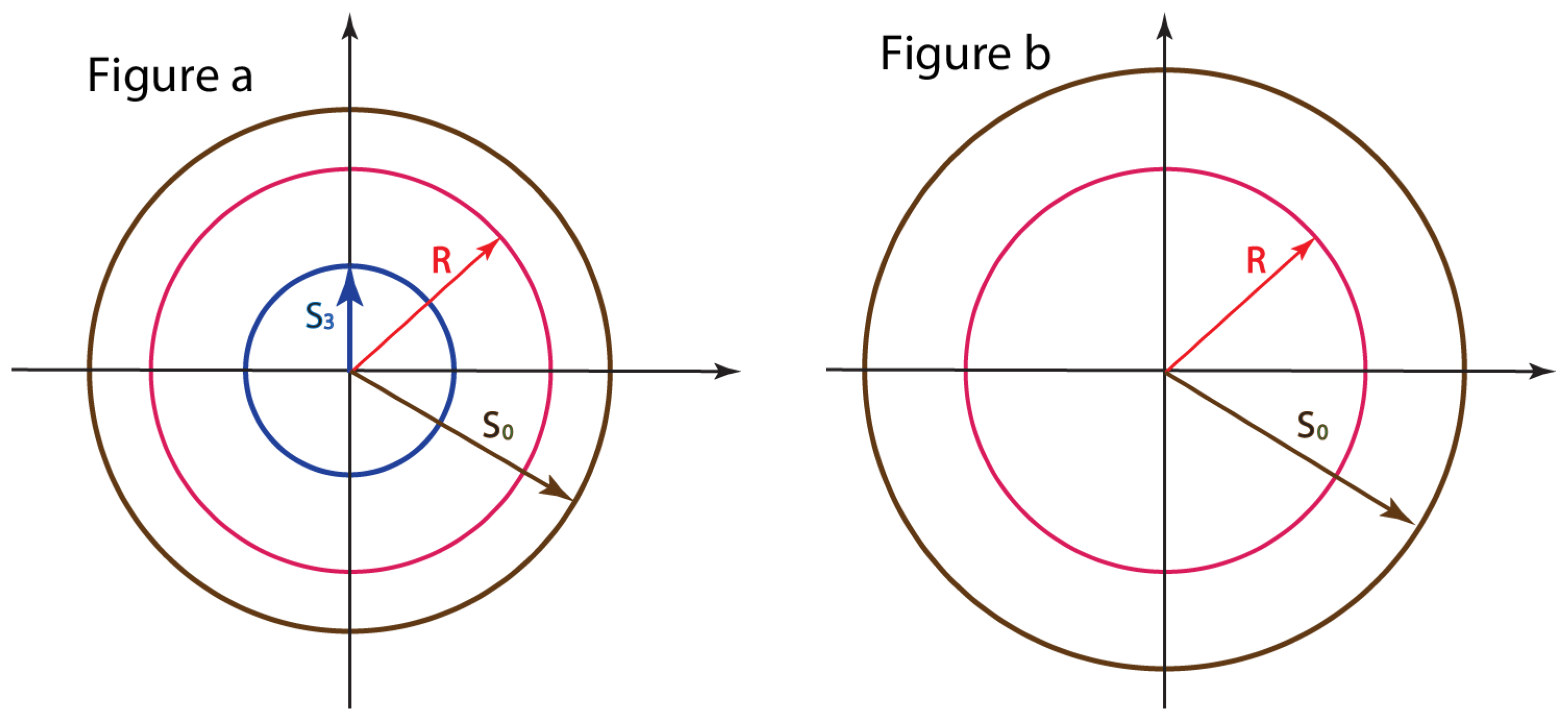
This aspect of the radius R is illustrated in Figure 1a. The minimum value of R is of Equation (64).
Figure 1.
Radius of the Poincaré sphere. The radius, R, takes its maximum value, , when the decoherence angle, χ, is zero. It becomes smaller as χ increases. It becomes minimum when the angle reaches 90°. Its minimum value is , as is illustrated in Figure a. The degree of polarization is maximum when and is minimum when . According to Equation (65), becomes zero when , and the minimum value of R becomes zero, as is indicated in Figure 1b. Its maximum value is still . This maximum radius can become larger because b becomes larger to make .
Let us go back to the four-momentum matrix of Equation (15). Its determinant is and remains invariant. Likewise, the determinant of the coherency matrix of Equation (58) should also remain invariant. The determinant in this case is:
This quantity remains invariant. This aspect is shown on the last row of Table 3.
Let us go back to Equation (49). This matrix changes the relative magnitude of the amplitudes, a and b. Thus, without loss of generality, we can study the Stokes parameters with . The coherency matrix then becomes:
Since the angle, δ, does not play any essential roles, we can let and write the coherency matrix as:
Then, the minimum radius, , and of Equation (62) and R of Equation (64) become:
respectively. The Poincaré sphere becomes simplified to that of Figure 1b. This Poincaré sphere allows R to decrease to zero.
The determinant of the above two-by-two matrix is:
Since the Lorentz transformation leaves the determinant invariant, the change in this χ variable is not a Lorentz transformation. It is of course possible to construct a larger group in which this variable plays a role in a group transformation [23], but in this paper, we are more interested in its role in a particle gaining a mass. With this point in mind, let us diagonalize the coherency matrix of Equation (69). Then it takes the form:
This form is the same as the four-momentum matrix given in Equation (41). There, we were not able to associate the variable, χ, with any known physical process or symmetry operations of the Lorentz group. Fortunately, in this section, we noted that this variable comes from the degree of decoherence in polarization optics.
6. Concluding Remarks
In this paper, we noted first that the group of Lorentz transformations can be formulated in terms of two-by-two matrices. This two-by-two formalism can also be used for transformations of the coherency matrix in polarization optics consisting of four Stokes parameters.
Thus, this set of the four parameters is like a Minkowskian four-vector under four-by-four Lorentz transformations. In order to accommodate all four Stokes parameters, we noted that the radius of the Poincaré sphere should be allowed to vary from its maximum value to its minimum, corresponding to the fully and minimal coherent cases.
As in the case of the particle mass, the decoherence parameter in the Stokes formalism is invariant under Lorentz transformations. However, the Poincaré sphere, with a variable radius, provides the mechanism for the variations of the decoherence parameter. It was noted that this variation gives a physical process whose mathematics correspond to that of the mass variable in particle physics.
As for polarization optics, the traditional approach has been to work with two polarizer matrices, like:
We have replaced these two matrices by one attenuation matrix of Equation (47). This replacement enables us to formulate the Lorentz group for the Stokes parameters [15]. Furthermore, this attenuation matrix makes it possible to make a continuous transformation from one matrix to another by adjusting the attenuation parameters in optical media. It could be interesting to design optical experiments along this direction.
Acknowledgments
This paper is in part based on an invited paper presented by one of the authors (YSK) at the Fedorov Memorial Symposium: International Conference “Spins and Photonic Beams at Interface”, dedicated to the 100th anniversary of F.I. Fedorov (1911–1994) (Minsk, Belarus, 2011). He would like to thank Sergei Kilin for inviting him to the conference.
In addition to numerous original contributions in optics, Fedorov wrote a book on two-by-two representations of the Lorentz group based on his own research on this subject. It was, therefore, quite appropriate for him (YSK) to present a paper on applications of the Lorentz group to optical science. He would like to thank V. A. Dluganovich and M. Glaynskii for bringing the papers and the book written by Academician Fedorov, as well as their own papers to his attention.
Conflict of Interest
The authors declare no conflict of interest.
Appendix
In Section 2, we listed four two-by-two matrices whose repeated applications lead to the most general form of the two-by-two matrix, G. It is known that every G matrix can be translated into a four-by-four Lorentz transformation matrix through [4,9,15]:
and:
These matrices appear to be complicated, but it is enough to study the matrices of Equation (13) and Equation (14) to cover all the matrices in this group. Thus, we give their four-by-four equivalents in this Appendix:
leads to the four-by-four matrix:
Likewise:
and:
References
- Azzam, R.A.M.; Bashara, I. Ellipsometry and Polarized Light; North-Holland: Amsterdam, The Netherlands, 1977. [Google Scholar]
- Born, M.; Wolf, E. Principles of Optics, 6th ed.; Pergamon: Oxford, NY, USA, 1980. [Google Scholar]
- Brosseau, C. Fundamentals of Polarized Light: A Statistical Optics Approach; John Wiley: New York, NY, USA, 1998. [Google Scholar]
- Naimark, M.A. Linear representation of the Lorentz group. Uspekhi Mater. Nauk 1954, 9, 19–93, Translated by Atkinson, F.V., American Mathematical Society Translations, Series 2, 1957, 6, 379–458. [Google Scholar]
- Naimark, M.A. Linear Representations of the Lorentz Group; Pergamon Press: Oxford, NY, USA, 1958; Translated by Swinfen, A.; Marstrand, O.J., 1964. [Google Scholar]
- Kim, Y.S.; Wigner, E.P. Space-time geometry of relativistic particles. J. Math. Phys. 1990, 31, 55–60. [Google Scholar] [CrossRef]
- Wigner, E. On unitary representations of the inhomogeneous Lorentz group. Ann. Math. 1939, 40, 149–204. [Google Scholar] [CrossRef]
- Kim, Y.S. Poincaré Sphere and Decoherence Problems. Available online: http://arxiv.org/abs/1203.4539 (accessed on 17 June 2013).
- Kim, Y.S.; Noz, M.E. Theory and Applications of the Poincaré Group; Reidel: Dordrecht, The Netherlands, 1986. [Google Scholar]
- Han, D.; Kim, Y.S.; Son, D. E(2)-like little group for massless particles and polarization of neutrinos. Phys. Rev. D 1982, 26, 3717–3725. [Google Scholar]
- Başkal, S.; Kim, Y.S. One analytic form for four branches of the ABCD matrix. J. Mod. Opt. 2010, 57, 1251–1259. [Google Scholar] [CrossRef]
- Başkal, S.; Kim, Y.S. Lorentz Group in Ray and Polarization Optics. In Mathematical Optics: Classical, Quantum and Computational Methods; Lakshminarayanan, V., Calvo, M.L., Alieva, T., Eds.; CRC Taylor and Francis: New York, NY, USA, 2013; Chapter 9; pp. 303–349. [Google Scholar]
- Saleh, B.E.A.; Teich, M.C. Fundamentals of Photonics, 2nd ed.; John Wiley: Hoboken, NJ, USA, 2007. [Google Scholar]
- Han, D.; Kim, Y.S.; Noz, M.E. Jones-vector formalism as a representation of the Lorentz group. J. Opt. Soc. Am. A 1997, 14, 2290–2298. [Google Scholar]
- Han, D.; Kim, Y.S.; Noz, M.E. Stokes parameters as a Minkowskian four-vector. Phys. Rev. E 1997, 56, 6065–6076. [Google Scholar]
- Feynman, R.P. Statistical Mechanics; Benjamin/Cummings: Reading, MA, USA, 1972. [Google Scholar]
- Han, D.; Kim, Y.S.; Noz, M.E. Illustrative example of Feynman’s rest of the universe. Am. J. Phys. 1999, 67, 61–66. [Google Scholar] [CrossRef]
- Pellat-Finet, P. Geometric approach to polarization optics. II. Quarternionic representation of polarized light. Optik 1991, 87, 68–76. [Google Scholar]
- Dlugunovich, V.A.; Kurochkin, Y.A. Vector parameterization of the Lorentz group transformations and polar decomposition of Mueller matrices. Opt. Spectrosc. 2009, 107, 312–317. [Google Scholar] [CrossRef]
- Tudor, T. Vectorial Pauli algebraic approach in polarization optics. I. Device and state operators. Optik 2010, 121, 1226–1235. [Google Scholar] [CrossRef]
- Fedorov, F.I. Vector parametrization of the Lorentz group and relativistic kinematics. Theor. Math. Phys. 1970, 2, 248–252. [Google Scholar] [CrossRef]
- Fedorov, F.I. Lorentz Group; [in Russian]; Global Science, Physical-Mathematical Literature: Moscow, Russia, 1979. [Google Scholar]
- Başkal, S.; Kim, Y.S. De Sitter group as a symmetry for optical decoherence. J. Phys. A 2006, 39, 7775–7788. [Google Scholar]
- Dargys, A. Optical Mueller matrices in terms of geometric algebra. Opt. Commun. 2012, 285, 4785–4792. [Google Scholar] [CrossRef]
- Pellat-Finet, P.; Basset, M. What is common to both polarization optics and relativistic kinematics? Optik 1992, 90, 101–106. [Google Scholar]
© 2013 by the authors; licensee MDPI, Basel, Switzerland. This article is an open access article distributed under the terms and conditions of the Creative Commons Attribution license (http://creativecommons.org/licenses/by/3.0/).
Share and Cite
MDPI and ACS Style
Kim, Y.S.; Noz, M.E. Symmetries Shared by the Poincaré Group and the Poincaré Sphere. Symmetry 2013, 5, 233-252. https://doi.org/10.3390/sym5030233
AMA Style
Kim YS, Noz ME. Symmetries Shared by the Poincaré Group and the Poincaré Sphere. Symmetry. 2013; 5(3):233-252. https://doi.org/10.3390/sym5030233
Chicago/Turabian StyleKim, Young S., and Marilyn E. Noz. 2013. "Symmetries Shared by the Poincaré Group and the Poincaré Sphere" Symmetry 5, no. 3: 233-252. https://doi.org/10.3390/sym5030233