1. Introduction
One-dimensional integer partition of periodic space into segments (of
mod N) containing k-points-atoms was proposed by Patterson [
1] and researched [
2,
3] to solve a homometrical theory problem that leads to the ambiguity of crystal structure interpretation. In particular, it was demonstrated [
4] that the vector system point disposition along the nodal directions of the orthogonal cell of
N ×
N nodes allows us to have a set of two-dimensional (2D) homometric structures for each direction. In that case, the vector system for each of these structures contains all points of the lattice constant
N. In combinatorics (
Table 3 [
5]), the coordinates of the structure of the complete vector system of points form a block diagram and (
v,
k,
λ)- difference set, where
v =
N-,
k- is the minimum number of points with integer coordinates and
λ- is the multiplicity of points in the vector system. When building a complete system of vector points in the two-dimensional lattice and the centered cells of the lattice, its versions form the basis of the discrete two-dimensional model, and the
n-dimensional packing space is formed
N times. The choice of direction in the lattice containing
N ×
N nodes defines one of the sublattices, and its cell is composed of
N lattice nodes.
Enumerating the options of homometric structures with a given number k (k + 1) = N of vector system points in the cell of a two-dimensional structure showed that this number coincides with (N + 1), but only for simple N. A solution of the general problem of enumerating the number of two-dimensional (2D) and three-dimensional (3D) lattices with N-nodes in the translational lattice was obtained after the introduction of the concept of packing space (PS) and its formalization.
Report [
6] had the goal of using PS for the search, generation and prediction of structures based on the partition of space into polyominoes. Some practical steps were used to establish the method of discrete modeling of partitions and packages [
7] to predict variations of molecular crystal structure (see, for example, [
8]). The basis of the method was the partition of periodic space into policubes (3D-polyomino).
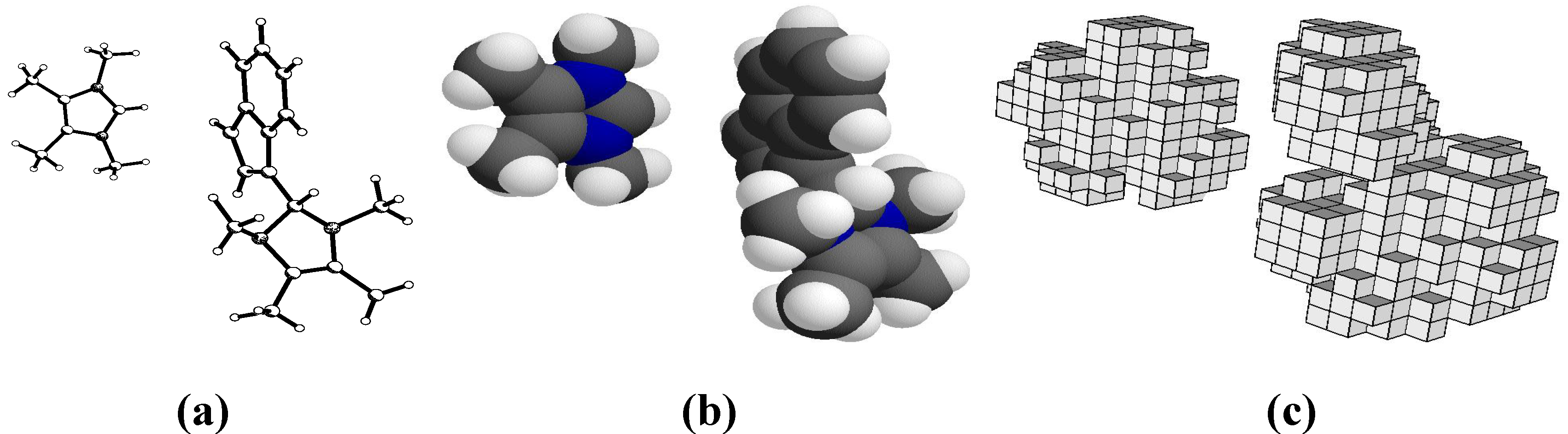
Figure 1 represents molecules in the form of policubes.
Figure 1.
(a) The rod model of molecules; (b) geometrical (spherical) model; and (c) discrete model (policube).
Figure 1.
(a) The rod model of molecules; (b) geometrical (spherical) model; and (c) discrete model (policube).
Generally, a growing number of publications have been devoted to the problems of the space partition (see for example [
9] or a collection dedicated to M. Gardner [
10]). Recent works published in
Symmetry [
11] were also concerned with the problems of space partition into polyominoes and polyiamonds.
The results represented in article [
11] show that the interest in partitions is not decreasing and that many problems have not yet been solved. Research carried out by a group of scientists from Vladimir State University (VlSU, Vladimir, Russia), described elsewhere [
7,
12], continues. To the best of our knowledge, this paper represents another way to partition periodic space into 2D-, 3D-polyomino with the help of final permutation groups never described before.
The presentation of a generalized packaging
N ×
N space containing all two-dimensional lattices of packing spaces of
Nth order was introduced in [
12]. Generalized criterion of the space partition into the polyominoes and policubes based on the Patterson model of structure as a vector system of points with integer values of the coordinates (in fractions of the cell) has been proposed. Algorithms and programs of the space partition into the polyominoes (2D), policubes (3D) and prediction of the model and actual molecular structures were partially presented in [
13,
14].
These investigations have proceeded in another direction in the description of the mechanism of the layered growth of real and model crystal structures [
15,
16].
The ideas of the approach are based on the research by Conway, Sloane,
et al. [
17]. The properties of the resulting 3D-packaging polyhedron (
Figure 2) in a mathematical model of the growing connection graph of the polyominoes in the partition have been studied and described in [
18,
19]. Article [
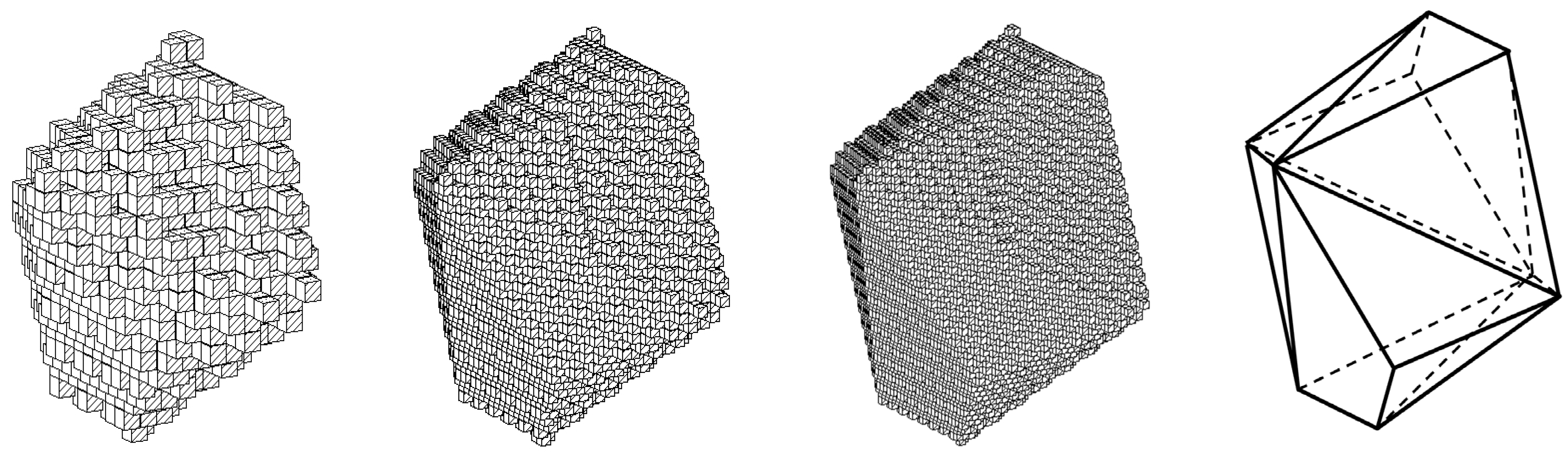
20] presented the results of the packing polyhedra calculation of growth in crystal nuclei of real structures (nanoclusters) of rhombic and monoclinic sulfur. The possibilities of using the Cambridge Structural Database (CSD) for a great number of nanoclusters of different molecular compounds were presented in [
20]. Anthracene, pentacene, coronene and halite nanoclusters were also researched. Based on the calculation of nanoclusters, a multicenter computer model of random nucleation and growth of crystal nuclei in the material has been developed. The output for the two-phase polycrystalline samples of monoclinic and rhombic sulfur S
8 is presented in
Figure 3. The sizes of the nuclei in the figure range from 1 nm to 8 nm.
Figure 2.
Formation of a grown polyhedron by tiling of the plane into policubes. The number of layers
n [
15] is consistently indicated (
n = 5;
n = 10;
n = 15).
Figure 2.
Formation of a grown polyhedron by tiling of the plane into policubes. The number of layers
n [
15] is consistently indicated (
n = 5;
n = 10;
n = 15).
Figure 3.
A multicenter model of the growth of monoclinic and rhombic sulfur S8 nanoclusters presented in “the Nanoscopic Computer”. Color of the clusters identifies various moments of the random nucleation of the future crystalline phases.
Figure 3.
A multicenter model of the growth of monoclinic and rhombic sulfur S8 nanoclusters presented in “the Nanoscopic Computer”. Color of the clusters identifies various moments of the random nucleation of the future crystalline phases.
The concept of
n-dimensional packing space was introduced in [
21]. In [
22], it was proposed to use a mathematical permutation group for the analysis of the symmetry of the packing space (PS). The crystallographic symmetry PS
2D based on classical symmetry transformations in the Weyl group was presented in [
23]. Broadened options to use the method for the description of fractal non-periodic partitions at present were shown in [
24].
In this paper, we describe new results of a discrete model of packing space usage for the visualization of abstract finite groups of substitutions, quaternions, Pauli matrices, Dirac matrices, and a description of the real two-dimensional layer structure.
2. Basic Concepts and Definitions
In crystallography, figures built on the basis of joining squares are called polyomino, on the basis of triangles are called “polyiamonds” and on the basis of hexagon are called polyhexes (see for example, [
11]). The shape of the square and cube has been chosen to describe the space partition for simplicity of algorithms and software partition implementation and continuity of these figures in the transition from two- to three-dimensional, and then to
n-dimensional space [
21]. Three-dimensional analogs of the triangle (tetrahedron) and hexagon (hexagonal bipyramid or prism) do not give simple partitions.
The figures compiled from the
N-unicellular-squares or cubes in E
3 so that each square (or cube) is adjacent to at least one neighbor that has a common side, are called polyominoes [
11] (3D-polyomino, or policube).
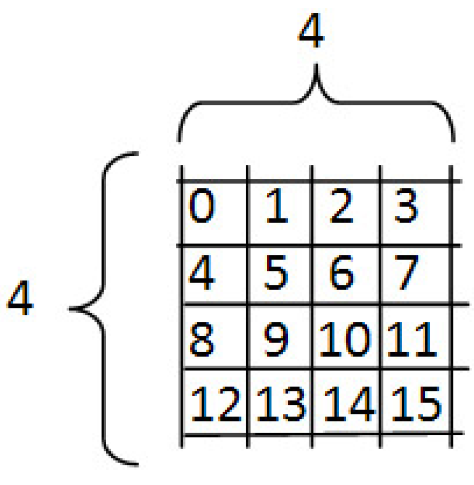
Figure 6 shows an example of figures “polyomino-cross” with
N = 5, which splits the space, that is, fills it without voids or overlays. It is evident that any
N-cellular polyomino can be fully presented on the plane in the area of the square containing the
N ×
N cells, each of which coincides with the size of the cells polyomino (
Figure 4, where
N = 6). Centers
N2 elementary cell of the square form
N2 nodes of the lattice translations of all the space. If the basic directions of space are used to select the horizontal and vertical lines, the nodes in this basis will have integer values (
Figure 4). The beginning of the reference in the chosen basis accept node is located in the upper left hand corner of the square. In the general case of not-primitive sublattice, this lattice, which has
N nodes, has a fundamental area of
N of the corresponding cells polyomino. The number of
N in this case is called the index of a sublattice or the order. Red (
Figure 4) highlights a nodal direction, determined by the translation of 0 → 8 that will be permutated in the cycles:
This is a permutation of highlights in the lattice of the series of parallel nodal lines (
Figure 4). Cell sublattice defines the coordinates of nodes: (6,0) and (2,1), but the fundamental area of the cell sublattice contains
N = 6 nodes, or 6 cells polyomino. The coordinates of the selected nodes can be represented in the form of vector-matrix columns:
and all the information about the selected cell sublattice is recorded as follows: PS-P 6 1
2, where the designation PS is a brief record of the “Pack Space”, and
P–plane. To partition, the policubes will use the symbol PS S, where S is the space—“Space”.
Figure 4.
A series of parallel nodal lines.
Figure 4.
A series of parallel nodal lines.
As sublattice in two-dimensional space is determined by two independent directions coming from the origin, the result was the following theorem:
Theorem 1. A beam translational independent nodal line conducted through the origin and every node of the square
N ×
N is a subgroup “
N2” of the permutations of the order of
N2. By forming a group of some of the directions in the lattice, it is simple, with the help of operations of multiplication, to find all of the subgroup “
N2” and its table Cayley. The result of this calculation for a simple case of
N = 4 is presented in
Table 1.
The splitting of the elements of the group on the equivalence classes that are defined as independent lines, and irreducible representations of the group “
N2”, which have the same color, is presented in the
Table 2. The number of directions is 16. The group is divided into 5 subgroups of 4 elements each, including the identity transformation. In each subgroup, operations are divided into cycles. Each cycle determines the number of equivalent nodes that form the sublattice translations. The number of cycles determines the number of independent nodes in the cell of the sublattice, which is the index of a sublattice.
From the geometry of the nodal lines in the space 4 × 4 (
Figure 5) and
Table 2, the operations of g(2), g(8) and g(10) are distinguished by one cell with an index of 8. Simple division of these cells into two independent parts leaves only two of them (g(10) and g(8)), each of which will be characterized by dividing the index, equal to 4. The remaining operations are divided into each subgroup to the equivalent of a pair, the number of which is equal to 5. Thus, the number of independent nodal areas is 7 for lattices with the index
N = 4, which coincides with the sum of the divisors of the number 4, as shown in the simple brute force of previously published works [
13].
Table 1.
Cayley table for N = 4.
Table 1.
Cayley table for N = 4.
| g[0]=(0 1 2 3 4 5 6 7 8 9 10 11 12 13 14 15 ); | g[0] | g[1] | g[2] | g[3] | g[4] | g[5] | g[6] | g[7] | g[8] | g[9] | g[10] | g[11] | g[12] | g[13] | g[14] | g[15] |
| g[1]=(5 6 7 4 9 10 11 8 13 14 15 12 1 2 3 0 ); | g[1] | g[2] | g[3] | g[0] | g[5] | g[6] | g[7] | g[4] | g[9] | g[10] | g[11] | g[8] | g[13] | g[14] | g[15] | g[12] |
| g[2]=(10 11 8 9 14 15 12 13 2 3 0 1 6 7 4 5 ); | g[2] | g[3] | g[0] | g[1] | g[6] | g[7] | g[4] | g[5] | g[10] | g[11] | g[8] | g[9] | g[14] | g[15] | g[12] | g[13] |
| g[3]=(15 12 13 14 3 0 1 2 7 4 5 6 11 8 9 10 ); | g[3] | g[0] | g[1] | g[2] | g[7] | g[4] | g[5] | g[6] | g[11] | g[8] | g[9] | g[10] | g[15] | g[12] | g[13] | g[14] |
| g[4]=(6 7 4 5 10 11 8 9 14 15 12 13 2 3 01); | g[4] | g[5] | g[6] | g[7] | g[8] | g[9] | g[10] | g[11] | g[12] | g[13] | g[14] | g[15] | g[0] | g[1] | g[2] | g[3] |
| g[5]=(11 8 9 10 15 12 13 14 3 0 1 2 7 4 5 6 ); | g[5] | g[6] | g[7] | g[4] | g[9] | g[10] | g[11] | g[8] | g[13] | g[14] | g[15] | g[12] | g[1] | g[2] | g[3] | g[0] |
| g[6]=(12 13 14 15 0 1 2 3 4 5 6 7 8 9 10 11 ); | g[6] | g[7] | g[4] | g[5] | g[10] | g[11] | g[8] | g[9] | g[14] | g[15] | g[12] | g[13] | g[2] | g[3] | g[0] | g[1] |
| g[7]=(1 2 3 0 5 6 7 4 9 10 11 8 13 14 15 12 ); | g[7] | g[4] | g[5] | g[6] | g[11] | g[8] | g[9] | g[10] | g[15] | g[12] | g[13] | g[14] | g[3] | g[0] | g[1] | g[2] |
| g[8]=(8 9 10 11 12 13 14 15 0 1 2 3 4 5 6 7 ); | g[8] | g[9] | g[10] | g[11] | g[12] | g[13] | g[14] | g[15] | g[0] | g[1] | g[2] | g[3] | g[4] | g[5] | g[6] | g[7] |
| g[9]=(13 14 15 12 1 2 3 0 5 6 7 4 9 10 11 8 ); | g[9] | g[10] | g[11] | g[8] | g[13] | g[14] | g[15] | g[12] | g[1] | g[2] | g[3] | g[0] | g[5] | g[6] | g[7] | g[4] |
| g[10]=(2 3 0 1 6 7 4 5 10 11 8 9 14 15 12 13 ); | g[10] | g[11] | g[8] | g[9] | g[14] | g[15] | g[12] | g[13] | g[2] | g[3] | g[0] | g[1] | g[6] | g[7] | g[4] | g[5] |
| g[11]=(7 4 5 6 11 8 9 10 15 12 13 14 3 0 1 2 ); | g[11] | g[8] | g[9] | g[10] | g[15] | g[12] | g[13] | g[14] | g[3] | g[0] | g[1] | g[2] | g[7] | g[4] | g[5] | g[6] |
| g[12]=(14 15 12 13 2 3 0 1 6 7 4 5 10 11 8 9 ); | g[12] | g[13] | g[14] | g[15] | g[0] | g[1] | g[2] | g[3] | g[4] | g[5] | g[6] | g[7] | g[8] | g[9] | g[10] | g[11] |
| g[13]=(3 0 1 2 7 4 5 6 11 8 9 10 15 12 13 14 ); | g[13] | g[14] | g[15] | g[12] | g[1] | g[2] | g[3] | g[0] | g[5] | g[6] | g[7] | g[4] | g[9] | g[10] | g[11] | g[8] |
| g[14]=(4 5 6 7 8 9 10 11 12 13 14 15 0 1 2 3 ); | g[14] | g[15] | g[12] | g[13] | g[2] | g[3] | g[0] | g[1] | g[6] | g[7] | g[4] | g[5] | g[10] | g[11] | g[8] | g[9] |
| g[15]=(9 10 11 8 13 14 15 12 1 2 3 0 5 6 7 4 ); | g[15] | g[12] | g[13] | g[14] | g[3] | g[0] | g[1] | g[2] | g[7] | g[4] | g[5] | g[6] | g[11] | g[8] | g[9] | g[10] |
Figure 5.
A series of parallel nodal lines.
Figure 5.
A series of parallel nodal lines.
Table 2.
The splitting of the elements of the group on the equivalence classes.
Table 2.
The splitting of the elements of the group on the equivalence classes.
| g[0] = (0 1 2 3 4 5 6 7 8 9 10 11 12 13 14 15 ) = (0) (1) (2) (3) (4) (5) (6) (7) (8) (9) (10) (11) (12) (13) (14) (15) |
| g[1] = (5 6 7 4 9 10 11 8 13 14 15 12 1 2 3 0 ) = |
| g[2] = (10 11 8 9 14 15 12 13 2 3 0 1 6 7 4 5 ) = (0 10) (1 11) (2 8) (3 9) (4 14) (5 15) ( 6 12) (7 13) |
| g[3] = (15 12 13 14 3 0 1 2 7 4 5 6 11 8 9 10 ) = |
| g[4] = (6 7 4 5 10 11 8 9 14 15 12 13 2 3 0 1 ) = |
| g[5] = (11 8 9 10 15 12 13 14 3 0 1 2 7 4 5 6 ) = |
| g[6] = (12 13 14 15 0 1 2 3 4 5 6 7 8 9 10 11 ) = |
| g[7] = (1 2 3 0 5 6 7 4 9 10 11 8 13 14 15 12 ) = |
| g[8] = (8 9 10 11 12 13 14 15 0 1 2 3 4 5 6 7 ) = (0 8) (1 9) (2 10) (3 11) (4 12) (5 13) (6 14) (7 15) |
| g[9] = (13 14 1 5 12 1 2 3 0 5 6 7 4 9 10 11 8 ) = |
| g[10] = (2 3 0 1 6 7 4 5 10 11 8 9 14 15 12 13 ) = (0 2) (1 3) (4 6) (5 7) (8 10) (9 11) (12 14) (13 15) |
| g[11] = (7 4 5 6 11 8 9 10 15 12 13 14 3 0 1 2 ) = |
| g[12] = (14 15 12 13 2 3 0 1 6 7 4 5 10 11 8 9 ) = |
| g[13] = (3 0 1 2 7 4 5 6 11 8 9 10 15 12 13 14 ) = |
| g[14] = (4 5 6 7 8 9 10 11 12 13 14 15 0 1 2 3 ) = |
| g[15] = (9 10 11 8 13 14 15 12 1 2 3 0 5 6 7 4 ) = |
Packing space (PS) or partition space is a lattice in which each node is assigned weight (symbol or color) so that any set of lattice nodes with the same weight makes the same (up to shift) sublattice of translations of the original lattice.
The columns of the vectors’ coordinates (based on the original lattice) of one of the sublattice bases of this lattice form an integral matrix:
where 0 ≤
x2 <
x1, 0 ≤
x3 <
x1, 0 ≤
y3 <
y2, and
z3 > 0.
Matrix Y is a matrix of three-dimensional packing space. The order of packing space coincides with the index of the sublattice and is the multiplication of the diagonal elements of the packing matrix N = x1y2z3.
For a two-dimensional lattice in the matrix, only numbers x1, x2, and y2 will remain. The order of the packing space in this case is N = x1y2.
For each node of the packing space, we construct a partition of the Dirichlet domains by dividing the interstitial distances by the median plane, and we obtain a partition of space into minimum areas that do not contain nodes, except one. These are cubes in three dimensions, and squares in the two dimensions (
Figure 6). In solid state physics, such lattice domains are called Wigner–Seitz cells. In [
25], the question of the structural organization of the complex compound with carbamide on the basis of the division of space into Dirichlet-polihedras was considered.
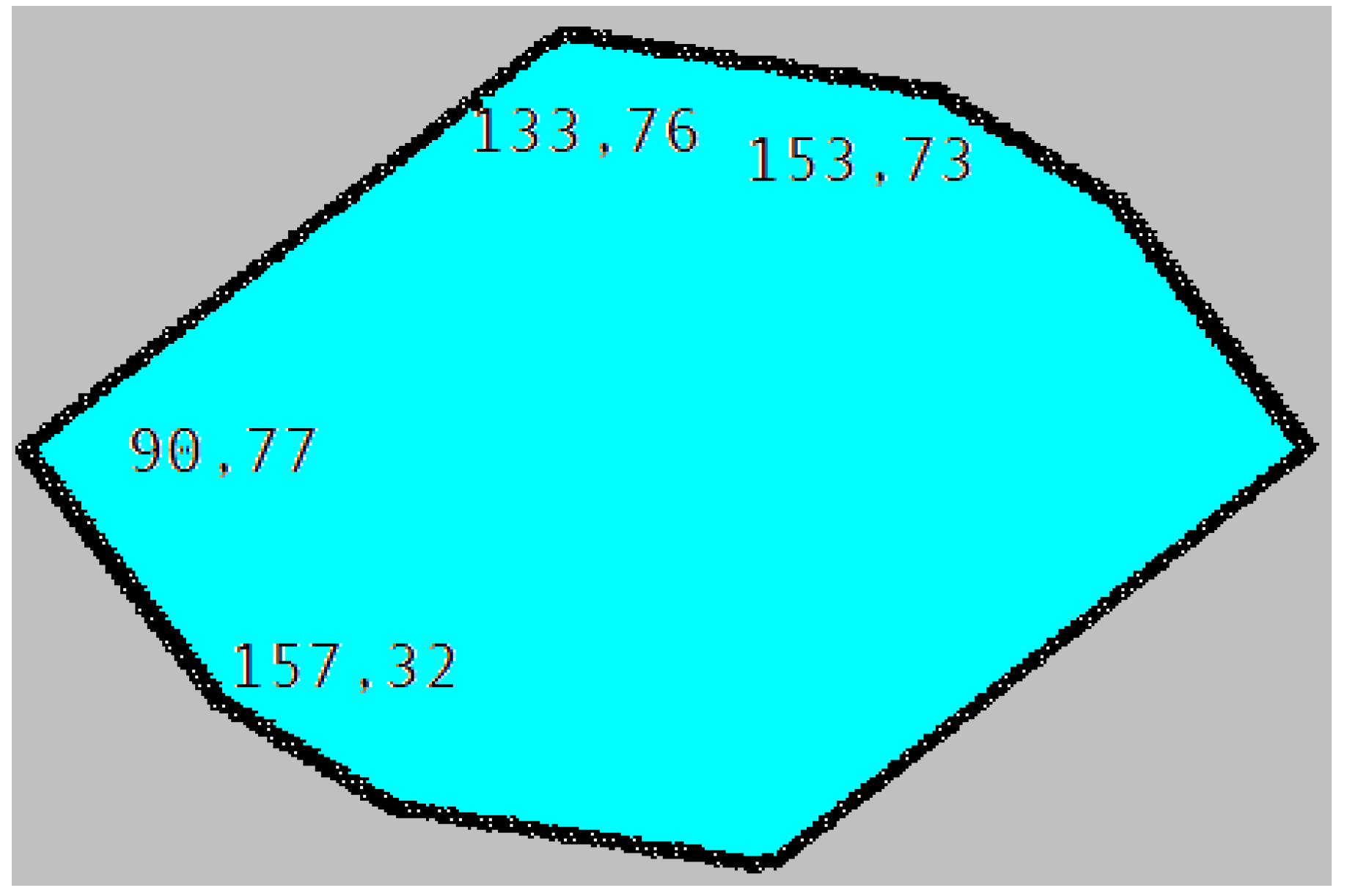
Figure 6.
Definition of the packing space. PS P 513.
Figure 6.
Definition of the packing space. PS P 513.
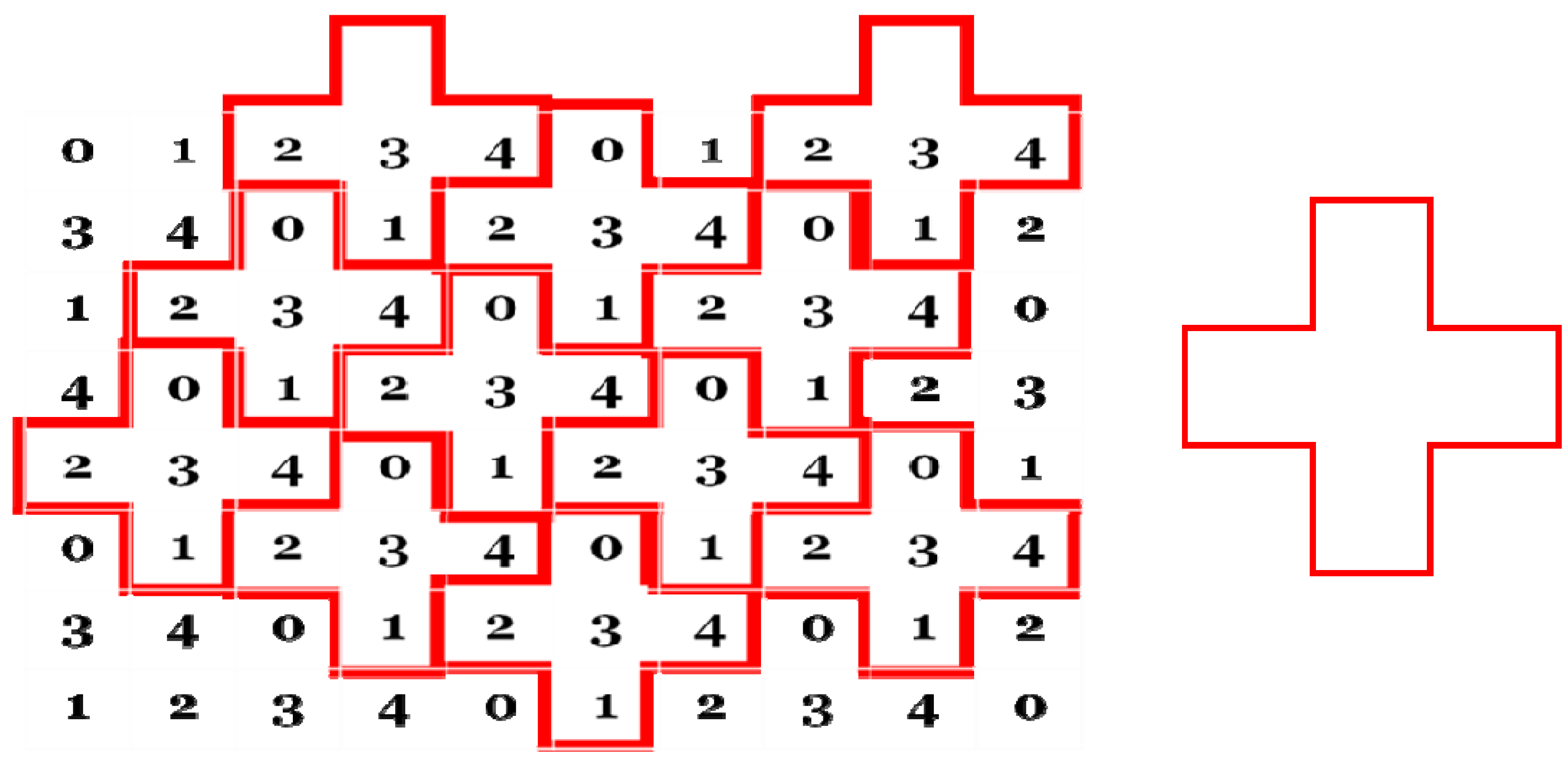
Let the size of the square coincide with the size of cells that make up the N-minoes of arbitrary shape. Then, we can address the problem of investing polyomino into the fundamental domain of two-dimensional packing space. If this can be conducted, the selected polyomino will tile space.
For example, we choose a polyomino of 5 cells in the form of a cross and put its middle cell with any of the packing spaces of P51
2 (
Figure 7). We assume the following statement (criterion of partition): if all the cells with the given orientation of the polyomino coincide with cells that have different weights in the packing space, the chosen polyomino breaks space. This conclusion is general and answers the question: Which polyomino (policube) or its assembly may become a fundamental domain of space partition?
Figure 7.
PS P512. One of the cells, corresponding to the range of PS, is selected by vectors. The criterion of the space partition is tested by the polyomino shape—the “cross”. The center of the figure coincides with the “weight 3” of PS.
Figure 7.
PS P512. One of the cells, corresponding to the range of PS, is selected by vectors. The criterion of the space partition is tested by the polyomino shape—the “cross”. The center of the figure coincides with the “weight 3” of PS.
The formalization of the basic concepts of the
n-dimensional packing space discrete model, policube and the partition criterion are given in [
21].
For the space presented in
Figure 6, we have
x1 = 5,
x2 = 3, and
y2 = 1. The two-dimensional packing space, presented in
Figure 3, is denoted as P5 1
3.
The number
N of packing spaces with a given order is finite and is determined by formula (1) [
7]:
For the image splitting, in addition to specifying the packaging space, each cell in the program of images in succession is encoded with the help of 4 characters: 0, 1, 2, 3. The first character is associated with the absence of the cells of the borders in the division. The following three are responsible for the existence of the border only on the left, only from the top and the left and top, respectively. The boundaries from the bottom and on the right are not taken into account because these limits are defined as cells, located below and to the right. The encoding of the cell structure, shown in
Figure 7, is recorded as follows: 3 1 3 0 2. On the encoding in the given packing space, all partitioning is restored. Procedure busting encoding characters and allocation in the division of areas with closed borders allow one to try all possible variants of partition space sublattice with the index
N. The code of the cell-neighbors is agreed upon so that the program can consistently surround each polyomino in the division of neighboring and find the structure of the layer-by-layer growth. In the computer experiment, it was found, and in [
18], strictly proved, that in the periodic partitioning the existence of a polygon growth (or growth of the polyhedron in three-dimensional space) is obligatory. Therefore, all of the crystals under ideal conditions grow up in the form of polyhedra.
Traditionally, analyzing a particular crystal structure, in accordance with the theorem (Cayley) about the isomorphism of an arbitrary finite group and the permutation group, for each type of crystallographic symmetry we can find an alternative compared to the transformation of space and the subgroup of permutations (Example 1.1 in this article), which is of academic interest. We proceed differently and apply the subgroup of permutations of the PS elements, and then, we perform the analysis of the resulting structure. Now, we have the first practical result immediately: If transformation is applied to the same PS, the resulting structures are geometrically conjugate to the periods and angles of the lattice in accordance with the concept of PS. This conjugation, in particular, is important for micro- and nano-electronics. Then, as each transformation of substitution can be represented in the form of cycles, each of them in the PS will match some domain that consists of equivalent points, and if we assign each set of equivalent points the same color, then we obtain space partitioned into separate fields. This is the second practical result. Partition models are important in the analysis of coordination packages in crystal chemistry. For every space partition, we can calculate packing polyhedron (polygon) of structure growth, the construction of which (by prescription [
15,
16]) helps us to determine how the number of dots on each layer of the growing shape varies (magic numbers) and how structural motives are arranged relating to faces (or edges) of the growth shape. This is the third practical result, which is used to construct models of nanoclusters [
20,
26].
To achieve these results, we compiled a program for sorting permutations with a given number of elements N, tiling into separate subgroups and construction of the Cayley table for each subgroup and presentation of the group operations in the form of cycles. An algorithm and program for each of the substitution operations to the packing space and the space partition into the colored areas were developed.
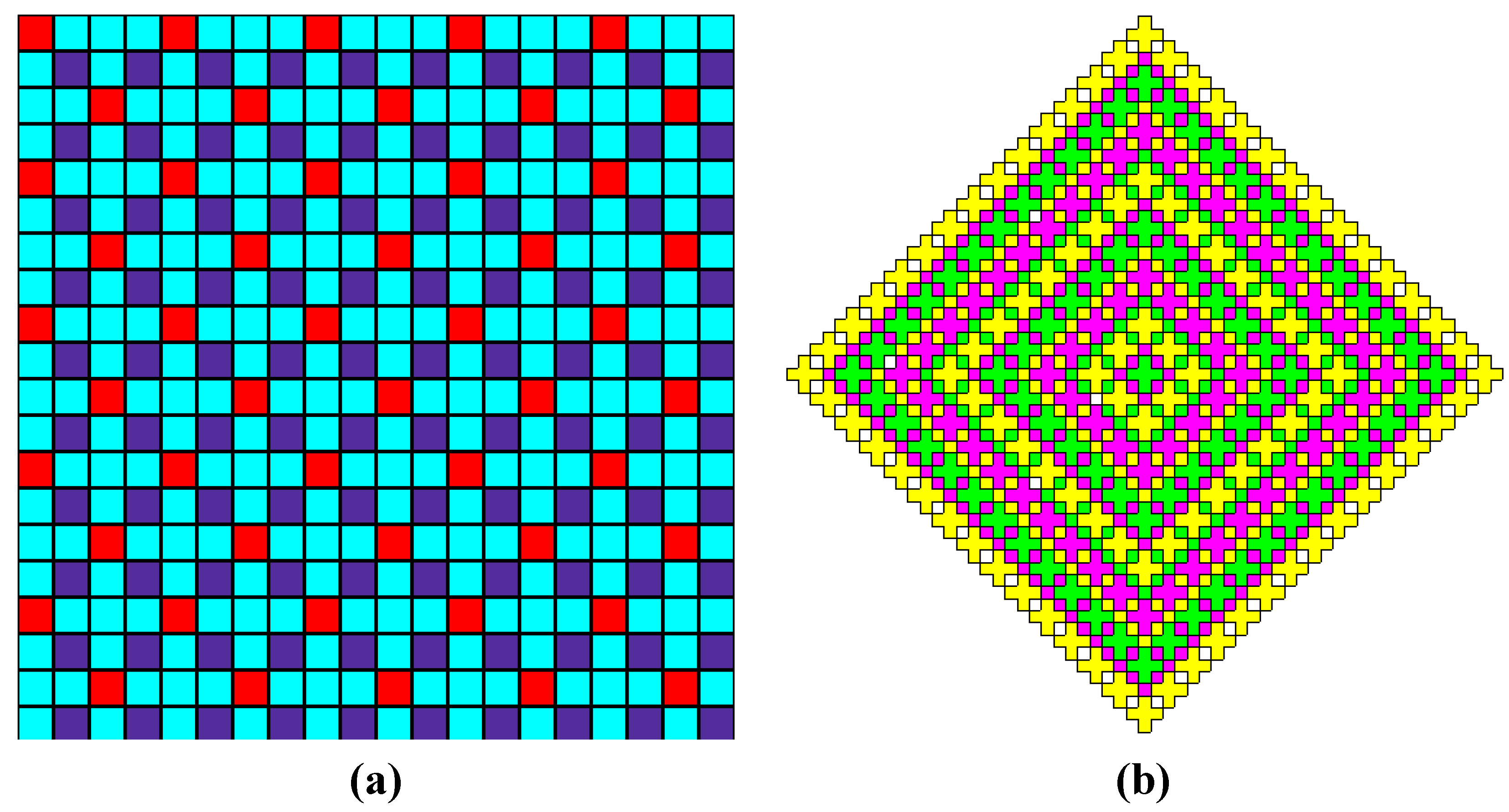
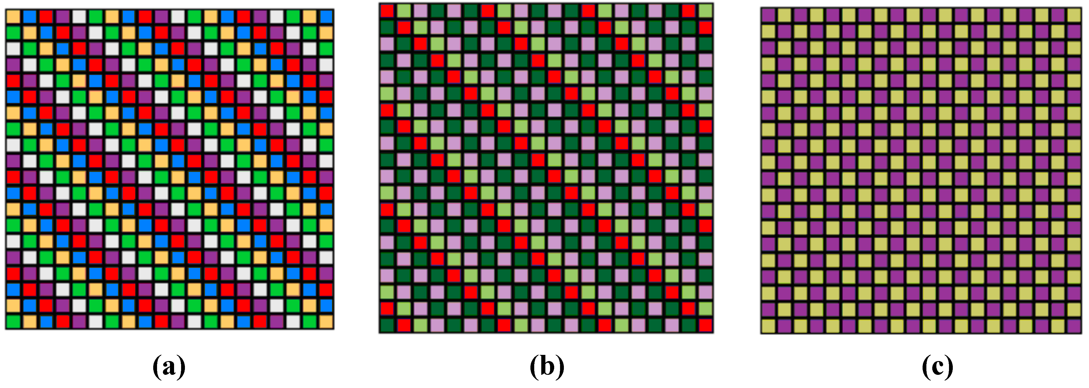
3. Examples of Permutation Groups on Packing Spaces
3.1. Arbitrary Permutation Groups
As an example, we analyze the structure of the partition on the symmetry plane of P4mm (
Figure 8). If you select symmetrically identical points of the structure and paint them one color (pick out point of the orbit), and then write the transformation of symmetry group with substitutions operations, you obtain eight operations, making up a group. A Cayley table of that group is presented in
Table 3. The group also includes the translation operation g(0), leaving all the points in their places. A column of
Table 3, delivered to the right of the Cayley table, presents the elements of points symmetry determined by the operations g(
N), which is written in the corresponding row.
Table 3.
Cayley table for the crystallographic group P4mm (
Figure 7).
Table 3.
Cayley table for the crystallographic group P4mm (Figure 7).
| g[0] = (0 1 2 3 4 5 6 7 ); | g[0] | g[1] | g[2] | g[3] | g[4] | g[5] | g[6] | g[7] | e |
| g[1] = (0 4 2 6 3 7 1 5 ); | g[1] | g[2] | g[3] | g[0] | g[5] | g[6] | g[7] | g[4] | 4 |
| g[2] = (0 3 2 1 6 5 4 7 ); | g[2] | g[3] | g[0] | g[1] | g[6] | g[7] | g[4] | g[5] | 2 |
| g[3] = (0 6 2 4 1 7 3 5 ); | g[3] | g[0] | g[1] | g[2] | g[7] | g[4] | g[5] | g[6] | 4 |
| g[4] = (0 1 2 3 6 7 4 5 ); | g[4] | g[7] | g[6] | g[5] | g[0] | g[3] | g[2] | g[1] | mh |
| g[5] = (0 6 2 4 3 5 1 7 ); | g[5] | g[4] | g[7] | g[6] | g[1] | g[0] | g[3] | g[2] | md1 |
| g[6] = (0 3 2 1 4 7 6 5 ); | g[6] | g[5] | g[4] | g[7] | g[2] | g[1] | g[0] | g[3] | mv |
| g[7] = (0 4 2 6 1 5 3 7 ); | g[7] | g[6] | g[5] | g[4] | g[3] | g[2] | g[1] | g[0] | md2 |
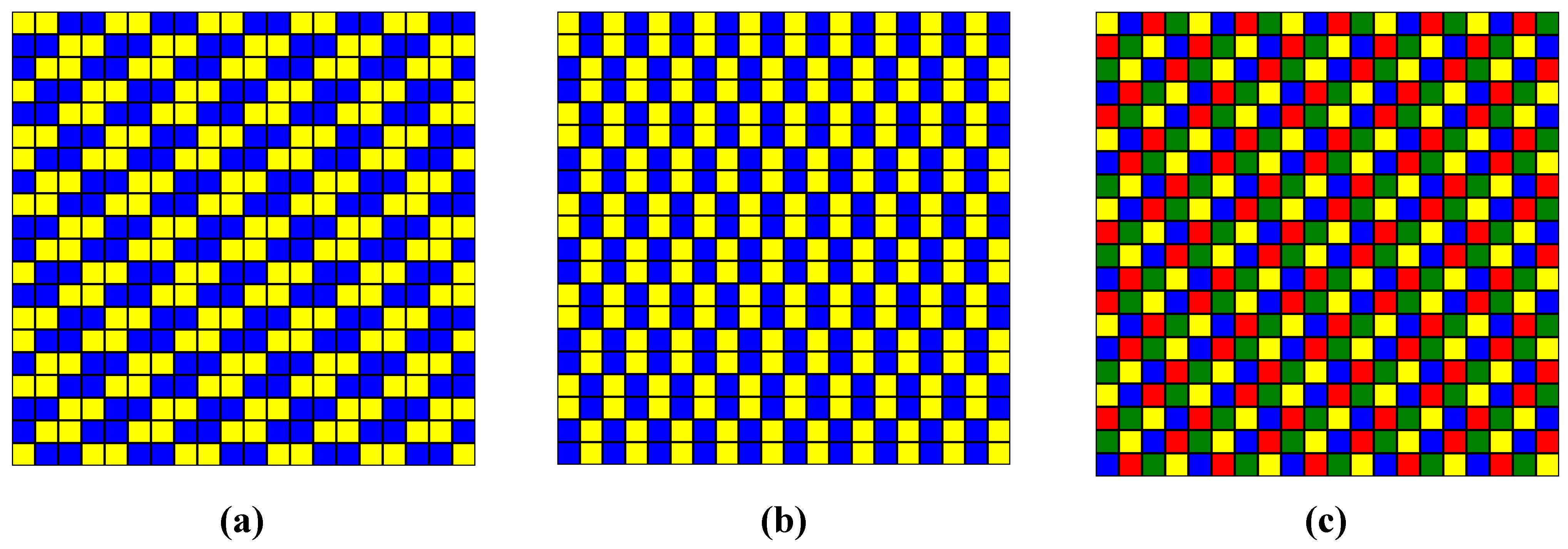
Another result with the other Cayley table is obtained when the cells belonging to each polyomino in the structure are painted the same color. In accordance with this approach,
Figure 8a shows the tri-colored structure, and its growth structure is shown in
Figure 8.
Figure 8.
(a) An example of P422 space partition into the polyomino and (b) the form of layered structure growth.
Figure 8.
(a) An example of P422 space partition into the polyomino and (b) the form of layered structure growth.
The corresponding 3-cycle transformation cannot be obtained in the group with the crystallographic operations presented in
Table 3. In the first case (
Table 3), we address the crystallographic operating space.
Table 4, in which the color is determined by the structure of the space tiling into the polyominoes, gives another representation of packing space. In this case, we assume that the space is the structural space. There is a variant, when these spaces are isomorphic, but it is obvious that the structural space is more general. Any crystallographic operational space defines a tiling of PS into polyominoes, but not every tiling is determined by the transformations of the operational space with the crystallographic symmetry of the plane (or space) group.
Table 4.
Cayley table for transformations PS P42
2 (for
Figure 8a).
Table 4.
Cayley table for transformations PS P422 (for Figure 8a).
| g[0] = (0 1 2 3 4 5 6 7 ) | g[0] | g[1] | g[2] | g[3] | g[4] | g[5] | g[6] | g[7] | g[8] | g[9] | 8-colored |
| g[1] = (0 2 3 4 6 7 1 5 ) | g[1] | g[2] | g[3] | g[4] | g[5] | g[6] | g[7] | g[8] | g[9] | g[0] | 3-colored |
| g[2] = (0 3 4 6 1 5 2 7 ) | g[2] | g[3] | g[4] | g[5] | g[6] | g[7] | g[8] | g[9] | g[0] | g[1] | 4-colored |
| g[3] = (0 4 6 1 2 7 3 5 ) | g[3] | g[4] | g[5] | g[6] | g[7] | g[8] | g[9] | g[0] | g[1] | g[2] | 3-colored |
| g[4] = (0 6 1 2 3 5 4 7 ) | g[4] | g[5] | g[6] | g[7] | g[8] | g[9] | g[0] | g[1] | g[2] | g[3] | 4-colored |
| g[5] = (0 1 2 3 4 7 6 5 ) | g[5] | g[6] | g[7] | g[8] | g[9] | g[0] | g[1] | g[2] | g[3] | g[4] | 7-colored |
| g[6] = (0 2 3 4 6 5 1 7 ) | g[6] | g[7] | g[8] | g[9] | g[0] | g[1] | g[2] | g[3] | g[4] | g[5] | 4-colored |
| g[7] = (0 3 4 6 1 7 2 5 ) | g[7] | g[8] | g[9] | g[0] | g[1] | g[2] | g[3] | g[4] | g[5] | g[6] | 3-colored |
| g[8] = (0 4 6 1 2 5 3 7 ) | g[8] | g[9] | g[0] | g[1] | g[2] | g[3] | g[4] | g[5] | g[6] | g[7] | 4-colored |
| g[9] = (0 6 1 2 3 7 4 5 ) | g[9] | g[0] | g[1] | g[2] | g[3] | g[4] | g[5] | g[6] | g[7] | g[8] | 3-colored |
In general, the second approach is characterized by non-crystallographic transformations of permutations.
To demonstrate the proposed method of analysis of any structure, including one with non-crystallographic symmetry, we consider a specific subgroup of permutations of the twelfth order. A Cayley table of the group is presented in
Table 5.
Table 5.
Cayley table for the subgroup of permutations of the twelfth order.
Table 5.
Cayley table for the subgroup of permutations of the twelfth order.
| g[0] | g[1] | g[2] | g[3] | g[4] | g[5] | g[6] | g[7] | g[8] | g[9] | g[10] | g[11] |
| g[1] | g[0] | g[3] | g[2] | g[5] | g[4] | g[7] | g[6] | g[9] | g[8] | g[11] | g[10] |
| g[2] | g[4] | g[0] | g[5] | g[1] | g[3] | g[8] | g[10] | g[6] | g[11] | g[7] | g[9] |
| g[3] | g[5] | g[1] | g[4] | g[0] | g[2] | g[9] | g[11] | g[7] | g[10] | g[6] | g[8] |
| g[4] | g[2] | g[5] | g[0] | g[3] | g[1] | g[10] | g[8] | g[11] | g[6] | g[9] | g[7] |
| g[5] | g[3] | g[4] | g[1] | g[2] | g[0] | g[11] | g[9] | g[10] | g[7] | g[8] | g[6] |
| g[6] | g[7] | g[8] | g[9] | g[10] | g[11] | g[0] | g[1] | g[2] | g[3] | g[4] | g[5] |
| g[7] | g[6] | g[9] | g[8] | g[11] | g[10] | g[1] | g[0] | g[3] | g[2] | g[5] | g[4] |
| g[8] | g[10] | g[6] | g[11] | g[7] | g[9] | g[2] | g[4] | g[0] | g[5] | g[1] | g[3] |
| g[9] | g[11] | g[7] | g[10] | g[6] | g[8] | g[3] | g[5] | g[1] | g[4] | g[0] | g[2] |
| g[10] | g[8] | g[11] | g[6] | g[9] | g[7] | g[4] | g[2] | g[5] | g[0] | g[3] | g[1] |
| g[11] | g[9] | g[10] | g[7] | g[8] | g[6] | g[5] | g[3] | g[4] | g[1] | g[2] | g[0] |
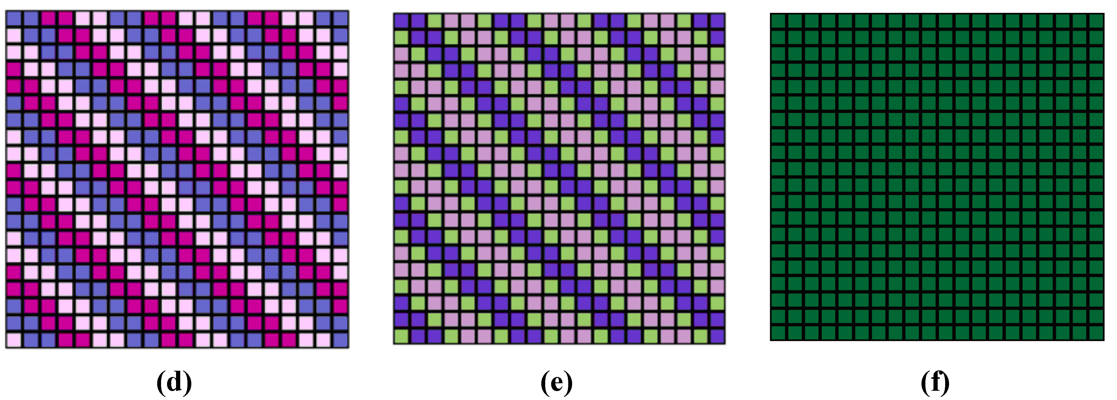
Multiplication of permutations allows the group to be split into classes of conjugate elements by iterating over the operations of multiplication, determining the conjugate elements by the rule:
As a result, we have 6 classes taken in braces:
{g(0)}; {g(1), g(2), g(5)}; {g(3), g(4)}; {g(6)}; {g(7), g(8) g(11)}; and {g(9), g(10)}.
The operations of substitutions and their cyclic representation, the number of colored areas in the PS P61
1 and distribution of the color designated by Latin letters in the layered structure of the packing space P61
1, are presented in
Table 6.
Table 6.
The operations of substitutions and their cyclic representation and the number of colored areas in the PS P611.
Table 6.
The operations of substitutions and their cyclic representation and the number of colored areas in the PS P611.
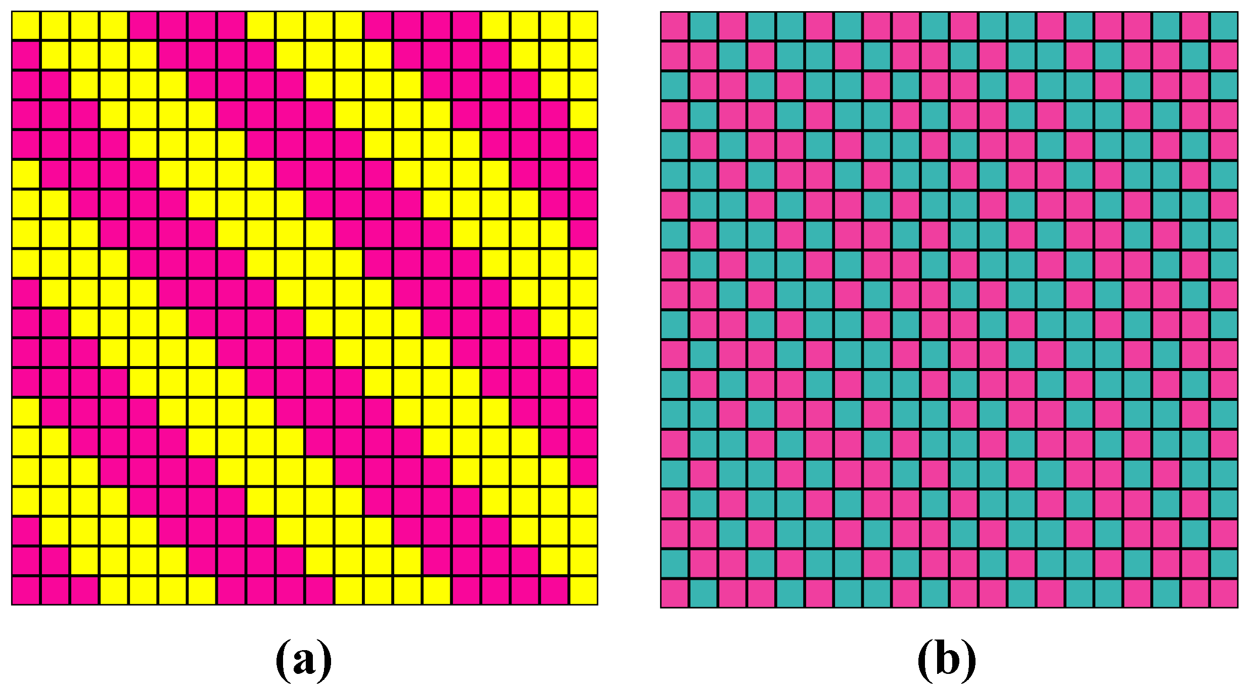
| Operations of substitutions | Cyclic representation | Number of colored areas | The alternation of layers in the PS P611 (Figure 9) |
|---|
| g[0] = (0 1 2 3 4 5 ) | (0)(1)(2)(3)(4)(5) | 6-colored | i j k l m n (Figure 9a) |
| g[1] = (0 1 4 5 2 3 ) | (0)(1)(24)(35) | 4-colored | i j i j k l (Figure 9b) |
| g[2] = (4 5 2 3 0 1 ) | (04)(15)(2)(3) | 4-colored | i j i j k l (Figure 9b) |
| g[3] = (4 5 0 1 2 3 ) | (042)(153) | 2-colored | i j i j i j (Figure 9c) |
| g[4] = (2 3 4 5 0 1 ) | (024)(135) | 2-colored | i j i j i j (Figure 9c) |
| g[5] = (2 3 0 1 4 5 ) | (02)(13)(4)(5) | 4-colored | i j i j k l (Figure 9b) |
| g[6] = (1 0 3 2 5 4 ) | (01)(23)(45) | 3-colored | i i j j k k (Figure 9d) |
| g[7] = (1 0 5 4 3 2 ) | (01)(25)(34) | 3-colored | i i j k k j (Figure 9e) |
| g[8] = (5 4 3 2 1 0 ) | (05)(14)(03) | 3-colored | i i j k k j (Figure 9e) |
| g[9] = (5 4 1 0 3 2 ) | (052143) | 1-colored | i i i i i i (Figure 9f) |
| g[10] = (3 2 5 4 1 0 ) | (034125) | 1-colored | i i i i i i (Figure 9f) |
| g[11] = (3 2 1 0 5 4 ) | (03)(12)(45) | 3-colored | i i j k k j (Figure 9e) |
Below (in
Figure 9 for P61
1), all independent structures are given. Under each of the colored variants, there are marked operations of the permutation groups applied to the PS in accordance with
Table 4, which replaces the numbering of figures.
Thus, there are only six independent colored PS P611 in the subgroup of permutations of the 12th order. Each variant matches its own class of conjugate group elements.
Figure 9.
Colored PS P611, obtained by partition of space by a subgroup of permutations of the 12th permutation order. (a) g(0); (b) g(1) = g(2) = g(5); (c) g(3) = g(4); (d) g(6); (e) g(7) = g(8) = g(11); (f) g(9) = g(10).
Figure 9.
Colored PS P611, obtained by partition of space by a subgroup of permutations of the 12th permutation order. (a) g(0); (b) g(1) = g(2) = g(5); (c) g(3) = g(4); (d) g(6); (e) g(7) = g(8) = g(11); (f) g(9) = g(10).
3.2. Quaternion Group D42
If the basis of the complex space are selected vectors:
as it is well known in mathematics, they will match the operational set, forming a two-dimensional representation:
Expressing the elements of representation set in terms of substitution, we have eight operations:
g(0) = 1= e = (0 1 2 3 4 5 6 7)= (0)(1)(2)(3)(4)(5)(6)(7)
g(1) = I = ( 2 3 1 0 7 6 4 5) = (0213)(4756)
g(2) = j = ( 4 5 6 7 1 0 3 2) = (0415)(2637)
g(3) = k = (6 7 5 4 2 3 1 0) = (0617)(2534)
g(4) = −1 = (1 0 3 2 5 4 7 6) = (01)(23)(45)(67)
g(5) = −I = (3 2 0 1 6 7 5 4) = (0312)(4657)
g(6) = −j = (5 4 7 6 0 1 2 3) = (0514)(2736)
g(7) = −k = (7 6 4 5 3 2 0 1) = (0716)(2435)
by simply composing permutation matrices, we can construct the following group Cayley table (
Table 7).
Table 7.
Cayley table for the quaternion group.
Table 7.
Cayley table for the quaternion group.
| 0 | 1 | 2 | 3 | 4 | 5 | 6 | 7 |
| 0 | 0 | 1 | 2 | 3 | 4 | 5 | 6 | 7 |
| 1 | 1 | 4 | 3 | 6 | 5 | 0 | 7 | 2 |
| 2 | 2 | 7 | 4 | 1 | 6 | 3 | 0 | 5 |
| 3 | 3 | 2 | 5 | 4 | 7 | 6 | 1 | 0 |
| 4 | 4 | 5 | 6 | 7 | 0 | 1 | 2 | 3 |
| 5 | 5 | 0 | 7 | 2 | 1 | 4 | 3 | 6 |
| 6 | 6 | 3 | 0 | 5 | 2 | 7 | 4 | 1 |
| 7 | 7 | 6 | 1 | 0 | 3 | 2 | 5 | 4 |
The symbols in the rows and columns of
Table 7 for each transformation of the group are replaced by the number corresponding to this transformation of permutation operation.
We will consider each row of
Table 7 as a new operation of substitution. It is easy to verify that the resulting new operating set will generate a group isomorphic to the quaternion group.
Table 8, derived from elements of rows 5, will have the properties of the original
Table 7.
Table 8.
Cayley table for the quaternion group.
Table 8.
Cayley table for the quaternion group.
| g[0] = (0 1 2 3 4 5 6 7 ) | g[0] | g[1] | g[2] | g[3] | g[4] | g[5] | g[6] | g[7] |
| g[1] = (2 7 4 1 6 3 0 5 ) | g[1] | g[2] | g[3] | g[0] | g[5] | g[6] | g[7] | g[4] |
| g[2] = (4 5 6 7 0 1 2 3 ) | g[2] | g[3] | g[0] | g[1] | g[6] | g[7] | g[4] | g[5] |
| g[3] = (6 3 0 5 2 7 4 1 ) | g[3] | g[0] | g[1] | g[2] | g[7] | g[4] | g[5] | g[6] |
| g[4] = (7 6 1 0 3 2 5 4 ) | g[4] | g[7] | g[6] | g[5] | g[2] | g[1] | g[0] | g[3] |
| g[5] = (1 4 3 6 5 0 7 2 ) | g[5] | g[4] | g[7] | g[6] | g[3] | g[2] | g[1] | g[0] |
| g[6] = (3 2 5 4 7 6 1 0 ) | g[6] | g[5] | g[4] | g[7] | g[0] | g[3] | g[2] | g[1] |
| g[7] = (5 0 7 2 1 4 3 6 ) | g[7] | g[6] | g[5] | g[4] | g[1] | g[0] | g[3] | g[2] |
We apply the same approach to the resulting Cayley
Table 8 again. However, despite the changed permutation operation workflow, the table view remains the same (
Table 9). Therefore, all operating sets obtained from the original group of quaternions are isomorphic, and any of them can be used to represent corresponding structures in the packing space.
Table 9.
Cayley table for the quaternion group.
Table 9.
Cayley table for the quaternion group.
| g[0] = (0 1 2 3 4 5 6 7 ) | g[0] | g[1] | g[2] | g[3] | g[4] | g[5] | g[6] | g[7] | (0)(1)(2)(3)(4)(5)(6)(7) |
| g[1] = (1 2 3 0 5 6 7 4 ) | g[1] | g[2] | g[3] | g[0] | g[5] | g[6] | g[7] | g[4] | (0123)(4567) |
| g[2] = (2 3 0 1 6 7 4 5 ) | g[2] | g[3] | g[0] | g[1] | g[6] | g[7] | g[4] | g[5] | (02)(13)(46)(57) |
| g[3] = (3 0 1 2 7 4 5 6 ) | g[3] | g[0] | g[1] | g[2] | g[7] | g[4] | g[5] | g[6] | (0321) (4765) |
| g[4] = (6 5 4 7 0 3 2 1 ) | g[4] | g[7] | g[6] | g[5] | g[2] | g[1] | g[0] | g[3] | (0426)(1735) |
| g[5] = (5 4 7 6 3 2 1 0 ) | g[5] | g[4] | g[7] | g[6] | g[3] | g[2] | g[1] | g[0] | (0527)(1436) |
| g[6] = (4 7 6 5 2 1 0 3 ) | g[6] | g[5] | g[4] | g[7] | g[0] | g[3] | g[2] | g[1] | (0624)(1537) |
| g[7] = (7 6 5 4 1 0 3 2 ) | g[7] | g[6] | g[5] | g[4] | g[1] | g[0] | g[3] | g[2] | (0725)(1634). |
Obviously, when we visualize the quaternion group, the order of the appropriate packing space should be a chosen multiple of the order of the permutations subgroup, that is, N = 8k. In this case, such as in Example 1.1, every cycle in an operation of the permutation subgroup selects in PS identical points (elementary squares, cubes), which are assigned a certain color. The whole space is divided into a number of one-colored, but differing from each other and in general unconnected colored areas, or into a number of corresponding substitution operation cycles. Thus, cycles determine the internal symmetry of the colored field.
Table 10.
Cayley table for the quaternion group.
Table 10.
Cayley table for the quaternion group.
| | g[1] | g[2] | g[3] | g[4] | g[5] | g[6] | g[7] |
| g[0] = (0 1 2 3 4 5 6 7 ) | g[0] | g[1] | g[2] | g[3] | g[4] | g[5] | g[6] | g[7] |
| g[1] = (1 6 3 4 5 2 7 0 ) | g[1] | g[2] | g[3] | g[0] | g[5] | g[6] | g[7] | g[4] |
| g[2] = (6 7 4 5 2 3 0 1 ) | g[2] | g[3] | g[0] | g[1] | g[6] | g[7] | g[4] | g[5] |
| g[3] = (7 0 5 2 3 4 1 6 ) | g[3] | g[0] | g[1] | g[2] | g[7] | g[4] | g[5] | g[6] |
| g[4] = (2 5 6 1 0 7 4 3 ) | g[4] | g[7] | g[6] | g[5] | g[2] | g[1] | g[0] | g[3] |
| g[5] = (5 4 1 0 7 6 3 2 ) | g[5] | g[4] | g[7] | g[6] | g[3] | g[2] | g[1] | g[0] |
| g[6] = (4 3 0 7 6 1 2 5 ) | g[6] | g[5] | g[4] | g[7] | g[0] | g[3] | g[2] | g[1] |
| g[7] = (3 2 7 6 1 0 5 4 ) | g[7] | g[6] | g[5] | g[4] | g[1] | g[0] | g[3] | g[2] |
Figure 10.
(a) PS 811, operation (01234567); (b) PS 811, operation (65470321).
Figure 10.
(a) PS 811, operation (01234567); (b) PS 811, operation (65470321).
Figure 11.
(a) PS 811, operation (12305674); (b) PS 811, operation (54763210).
Figure 11.
(a) PS 811, operation (12305674); (b) PS 811, operation (54763210).
Figure 12.
(a) PS 811, operation (23016745); (b) PS 811, operation (47652103).
Figure 12.
(a) PS 811, operation (23016745); (b) PS 811, operation (47652103).
Figure 13.
(a) PS 811, operation (30127456); (b) PS 811, operation (76541032).
Figure 13.
(a) PS 811, operation (30127456); (b) PS 811, operation (76541032).
Figure 14.
Quaternion group of P421 in the packing space. (a) The equivalent transformations of the group: (1 6 3 4 5 2 7 0) = (3 2 7 6 1 0 5 4) = (5 4 1 0 7 6 3 2) = (7 0 5 2 3 4 1 6); (b) the equivalent transformations of the group (2 5 6 1 0 7 4 3) = (4 3 0 7 6 1 2 5); (c) (6 7 4 5 2 3 0 1).
Figure 14.
Quaternion group of P421 in the packing space. (a) The equivalent transformations of the group: (1 6 3 4 5 2 7 0) = (3 2 7 6 1 0 5 4) = (5 4 1 0 7 6 3 2) = (7 0 5 2 3 4 1 6); (b) the equivalent transformations of the group (2 5 6 1 0 7 4 3) = (4 3 0 7 6 1 2 5); (c) (6 7 4 5 2 3 0 1).
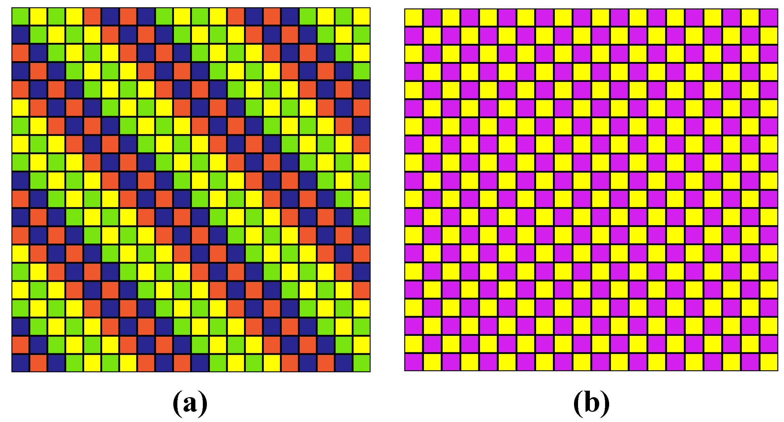
In packing space, the P81
1 quaternion group of symmetry is represented by a set of 8 structures. Among them, there is one representation of the operation of identical 8-colored transformation g(0) = (0) (1) (2) (3) (4) (5) (6) (7) (
Figure 10a), one 4-colored transformation operation g(1) = (02) (13) (46) (57) (
Figure 12a) and six two-colored transformation operations, dividing space into three pairs of equivalent structures. Thus, there are only five independent structures that correspond to the five classes of quaternions:
and consequently, the group has five irreducible representations. From a geometrical point of view, the quaternion group splits PS P81
1 into heterolayers (see, for example,
Figure 7,
Figure 8,
Figure 9,
Figure 10 and
Figure 11) and P42
1 into regions in the form of polyomino. There is a “degeneration” of permutation transformations in PS P42
1: (1 6 3 4 5 2 7 0), (3 2 7 6 1 0 5), (5 4 1 0 7 6 3 2 4), (7 0 5 2 3 4 1 6), which gives the same result. Thus, the structure of the packing space affects the number of independent partitions.
The transition between structures that are determined by one fixed operation of the permutation group, belonging to different packing spaces of the same order N, is discrete due to changes in the angular parameters of the sublattices. More information will be shown below in Example 1.6. Therefore, we can assume that the lattice is deformed in such a transition, and matrices of packing space function as a discrete deformation transformation (DDT). The number N of these transformations is finite and determined by (1).
3.3. Quaternion Group at the Extended Packing Space
Quaternion groups in the packing spaces of higher order can be used. We consider this possibility in the 16th order PS. We match two (or more) cells of packing space to each number in the record of quaternion group permutation transformations. As the number of characters that determine the quaternion group is 8, the order of packing space becomes equal to N = 16. A correspondence table of old and new characters can be selected on the basis of a simple ordered set of numbers:
0 = (0,1); 1 = (2,3); 2 = (4,5); 3 = (6,7); 4 = (8,9); 5 = (10,11); 6 = (12,13); and 7 = (14,15)
The subsequent note of new permutation operations and their cyclic partitions will appear as follows:
1H(0 1 2 3 4 5 6 7 8 9 10 11 12 13 14 15) = (0)(1)(2)(3)(4)(5)(6)(7)(8)(9)(10)(11)(12)(13)(14)(15);
iH (4 5 6 7 2 3 0 1 14 15 12 13 8 9 10 11) = (0 4 2 6)(1 5 3 7)(8 14 10 12)(9 15 11 13);
jH(8 9 10 11 12 13 14 15 2 3 0 1 6 7 4 5) = (0 8 2 10)(1 9 3 11)(4 12 6 14)(5 13 7 15);
kH(12 13 14 15 10 11 8 9 4 5 6 7 2 3 0 1) = (0 12 2 14)(1 13 3 15)(4 10 6 8)(5 11 7 9);
−1H(2 3 0 1 6 7 4 5 10 11 8 9 14 15 12 13) = (0 2)(1 3)(4 6)(5 7)(8 10)(9 11)(12 14)(13 15);
−iH(6 7 4 5 0 1 2 3 12 13 14 15 10 11 8 9) = (0 6 2 4)(1 7 3 5)(8 12 10 14)(9 13 11 15);
−jH(10 11 8 9 14 15 12 13 0 1 2 3 4 5 6 7) = (0 10 2 8)(1 11 3 9)(4 14 6 12)(5 15 7 13);
−kH(14 15 12 13 8 9 10 11 6 7 4 5 0 1 2 3) = (0 14 2 12)(1 15 3 13)(4 8 6 10)(5 9 7 11).
You can check that by simple multiplication of these operations, constructed in such a way that a new table will be identical to the original Cayley table of the quaternion group; the symmetry groups of packing spaces of the 8th and 16th order are isomorphic.
To compare colored structures PS P161
1 and PS P81
1, we choose operations i
H and i, and then, we present the results of their application to selected packing spaces (
Figure 15).
Figure 15.
Compliance of the quaternion symmetry group and dual quaternions in PS: (a) P811 (2 3 1 0 7 6 4 5); (b) PS P16 11 (4 5 6 7 2 3 0 1 14 15 12 13 89 10 11).
Figure 15.
Compliance of the quaternion symmetry group and dual quaternions in PS: (a) P811 (2 3 1 0 7 6 4 5); (b) PS P16 11 (4 5 6 7 2 3 0 1 14 15 12 13 89 10 11).
The heterolayers symmetry of selected structures is clear in the figures. This example shows that it is possible to increase the size of the structure while maintaining symmetry.
3.4. The Pauli Matrices Group
We apply the technique for imaging the symmetry group with the help of packing spaces to Pauli matrices, which are well known in physics. For this purpose, we will expand their number to the total subgroup, using the operation of matrices multiplication. The operation of the Pauli matrices multiplication in quantum mechanics is defined and leads to the commutation relations.
The Pauli matrices group is a subgroup of the order 16:
As a result, we obtain the following Cayley table for the Pauli matrices group (
Table 11).
Table 11.
Cayley table for the Pauli matrices group.
Table 11.
Cayley table for the Pauli matrices group.
| g(i) | [0] | [1] | [2] | [3] | [4] | [5] | [6] | [7] | [8] | [9] | [10] | [11] | [12] | [13] | [14] | [15] |
| [0] | [0] | [1] | [2] | [3] | [4] | [5] | [6] | [7] | [8] | [9] | [10] | [11] | [12] | [13] | [14] | [15] |
| [1] | [1] | [0] | [5] | [6] | [7] | [2] | [3] | [4] | [9] | [8] | [11] | [10] | [13] | [12] | [15] | [14] |
| [2] | [2] | [5] | [0] | [8] | [12] | [1] | [9] | [13] | [3] | [6] | [15] | [14] | [4] | [7] | [11] | [10] |
| [3] | [3] | [6] | [9] | [0] | [10] | [8] | [1] | [11] | [5] | [2] | [4] | [7] | [14] | [15] | [12] | [13] |
| [4] | [4] | [7] | [13] | [11] | [0] | [12] | [10] | [1] | [15] | [14] | [6] | [3] | [5] | [2] | [9] | [8] |
| [5] | [5] | [2] | [1] | [9] | [13] | [0] | [8] | [12] | [6] | [3] | [14] | [15] | [7] | [4] | [10] | [11] |
| [6] | [6] | [3] | [8] | [1] | [11] | [9] | [0] | [10] | [2] | [5] | [7] | [4] | [15] | [14] | [13] | [12] |
| [7] | [7] | [4] | [12] | [10] | [1] | [13] | [11] | [0] | [14] | [15] | [3] | [6] | [2] | [5] | [8] | [9] |
| [8] | [8] | [9] | [6] | [2] | [15] | [3] | [5] | [14] | [1] | [0] | [12] | [13] | [11] | [10] | [4] | [7] |
| [9] | [9] | [8] | [3] | [5] | [14] | [6] | [2] | [15] | [0] | [1] | [13] | [12] | [10] | [11] | [7] | [4] |
| [10] | [10] | [11] | [15] | [7] | [3] | [14] | [4] | [6] | [13] | [12] | [1] | [0] | [8] | [9] | [2] | [5] |
| [11] | [11] | [10] | [14] | [4] | [6] | [15] | [7] | [3] | [12] | [13] | [0] | [1] | [9] | [8] | [5] | [2] |
| [12] | [12] | [13] | [7] | [14] | [2] | [4] | [15] | [5] | [10] | [11] | [9] | [8] | [1] | [0] | [6] | [3] |
| [13] | [13] | [12] | [4] | [15] | [5] | [7] | [14] | [2] | [11] | [10] | [8] | [9] | [0] | [1] | [3] | [6] |
| [14] | [14] | [15] | [11] | [12] | [9] | [10] | [13] | [8] | [4] | [7] | [2] | [5] | [6] | [3] | [1] | [0] |
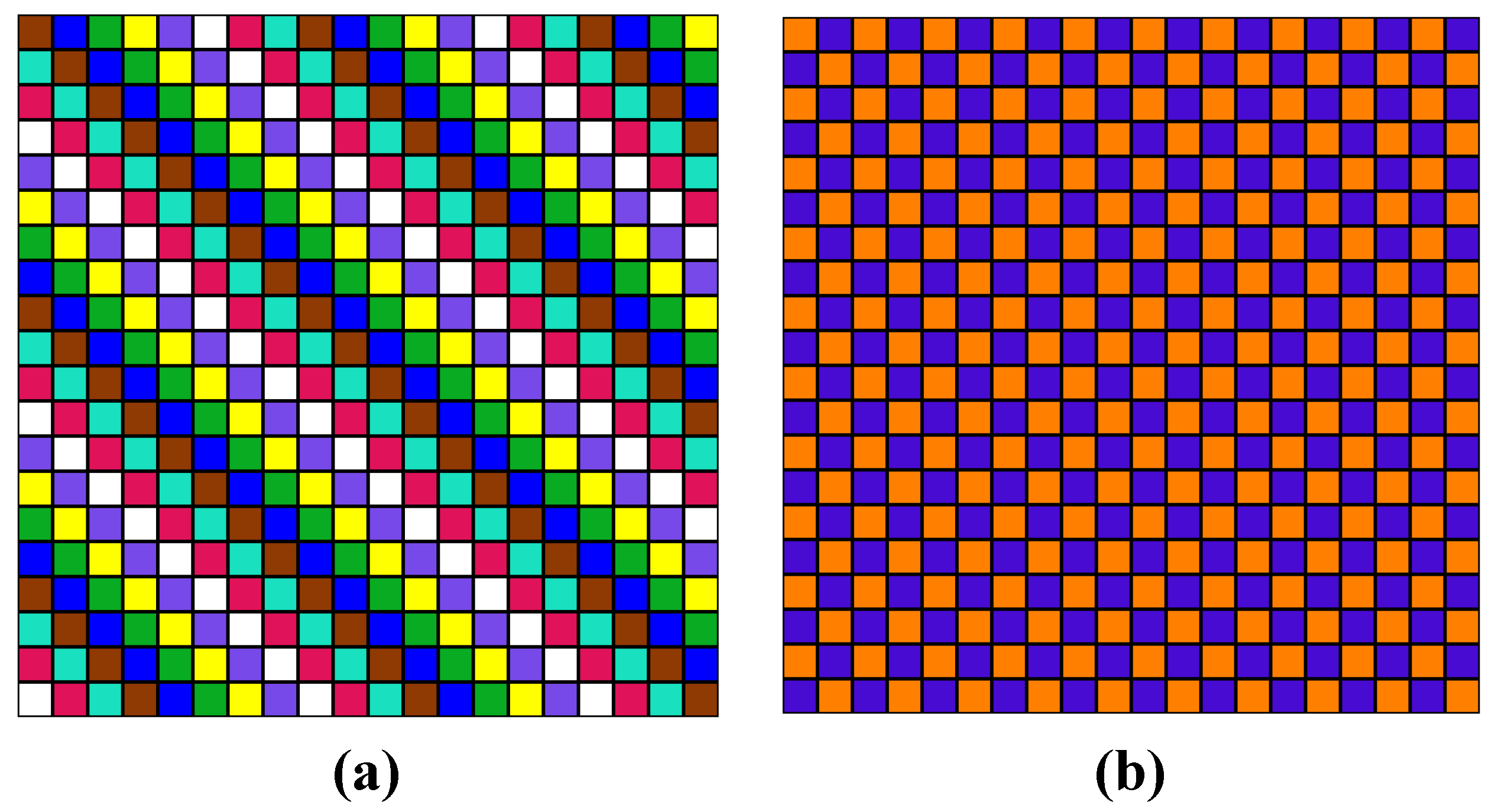
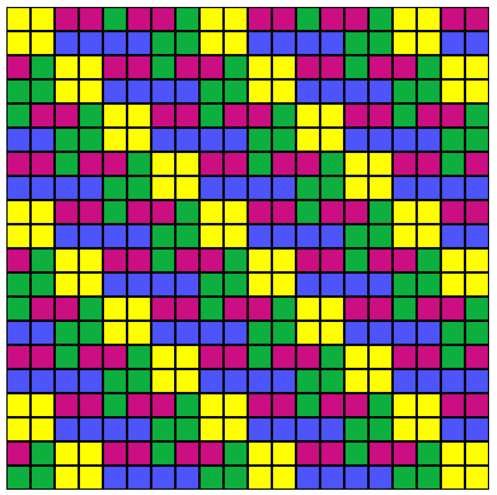
We choose to visualize a 4-color transformation g(8) = (8 9 6 2 15 3 5 14 1 0 12 13 11 10 4 7) = (0819) (2653) (4 15 7 14) (10 12 11 13) in the packing space P82
2. The result is presented in
Figure 16.
Figure 16.
Partition of PS P822 by element g(8) of the Pauli matrices permutation group.
Figure 16.
Partition of PS P822 by element g(8) of the Pauli matrices permutation group.
Package code in the program partition into polyomino (at [
7]): 3232132310322230.
Layer growth leads to the growth of shape in the form of a parallelogram, which is also characterized by an element of the Pauli matrices group (
Figure 17).
The sequence of growth is demonstrated on the diagram in
Figure 18. Numerical information is placed on the three linear functions, which correspond to the layer-growth studies of partition into polyomino and other pieces of plane periodic mosaics [
16,
17].
Figure 17.
The shape of the growth of the partition PS P822 by element of g(8) of the permutation group of the Pauli matrices.
Figure 17.
The shape of the growth of the partition PS P822 by element of g(8) of the permutation group of the Pauli matrices.
Figure 18.
Coordination (magic) numbers of layer growth structure.
Figure 18.
Coordination (magic) numbers of layer growth structure.
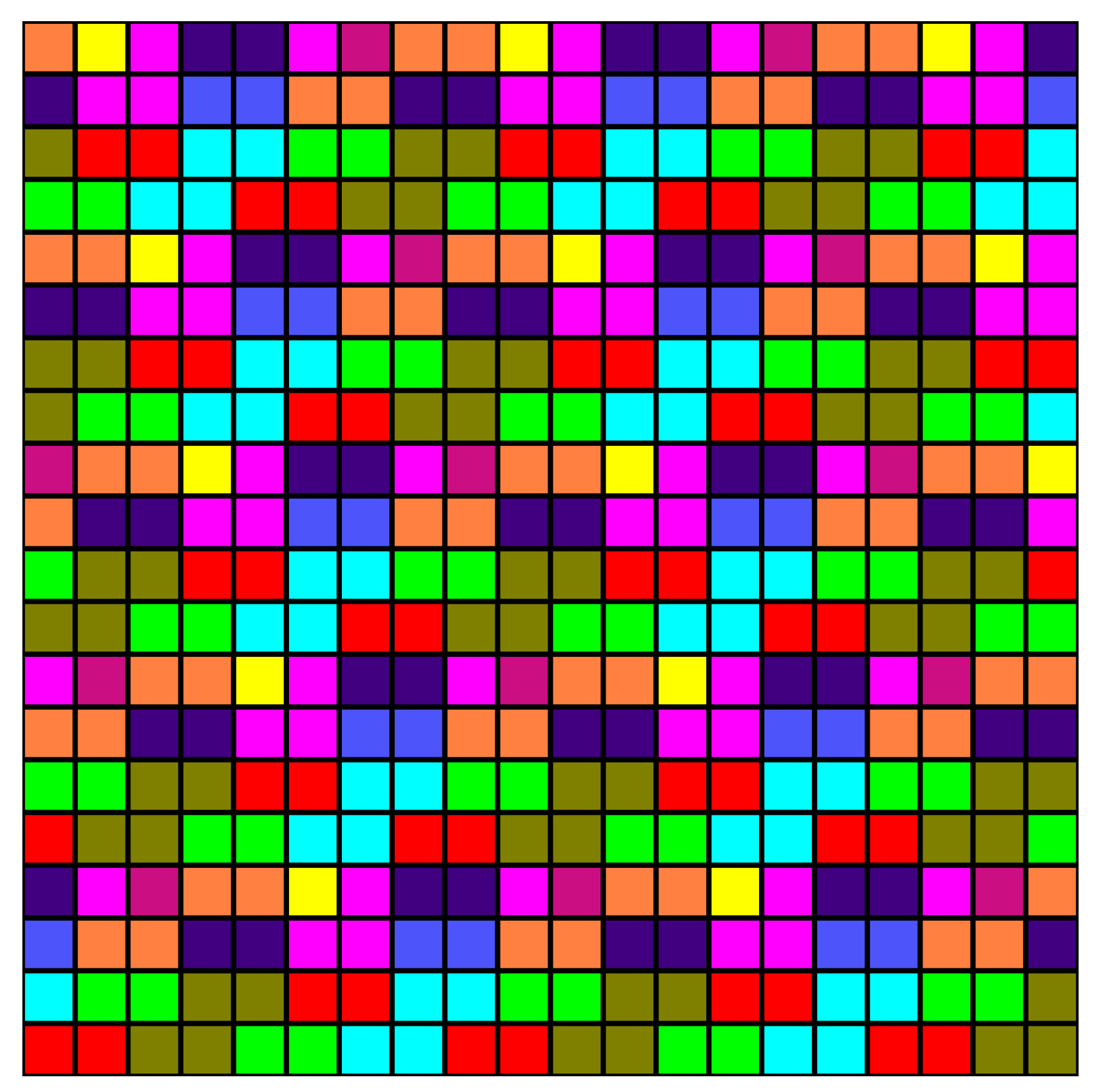
3.5. The Dirac Matrices Group
Similarly, we proceed with the Dirac matrices. The number of elements in the full group was found to be 32 with the Cayley table shown in
Table 12.
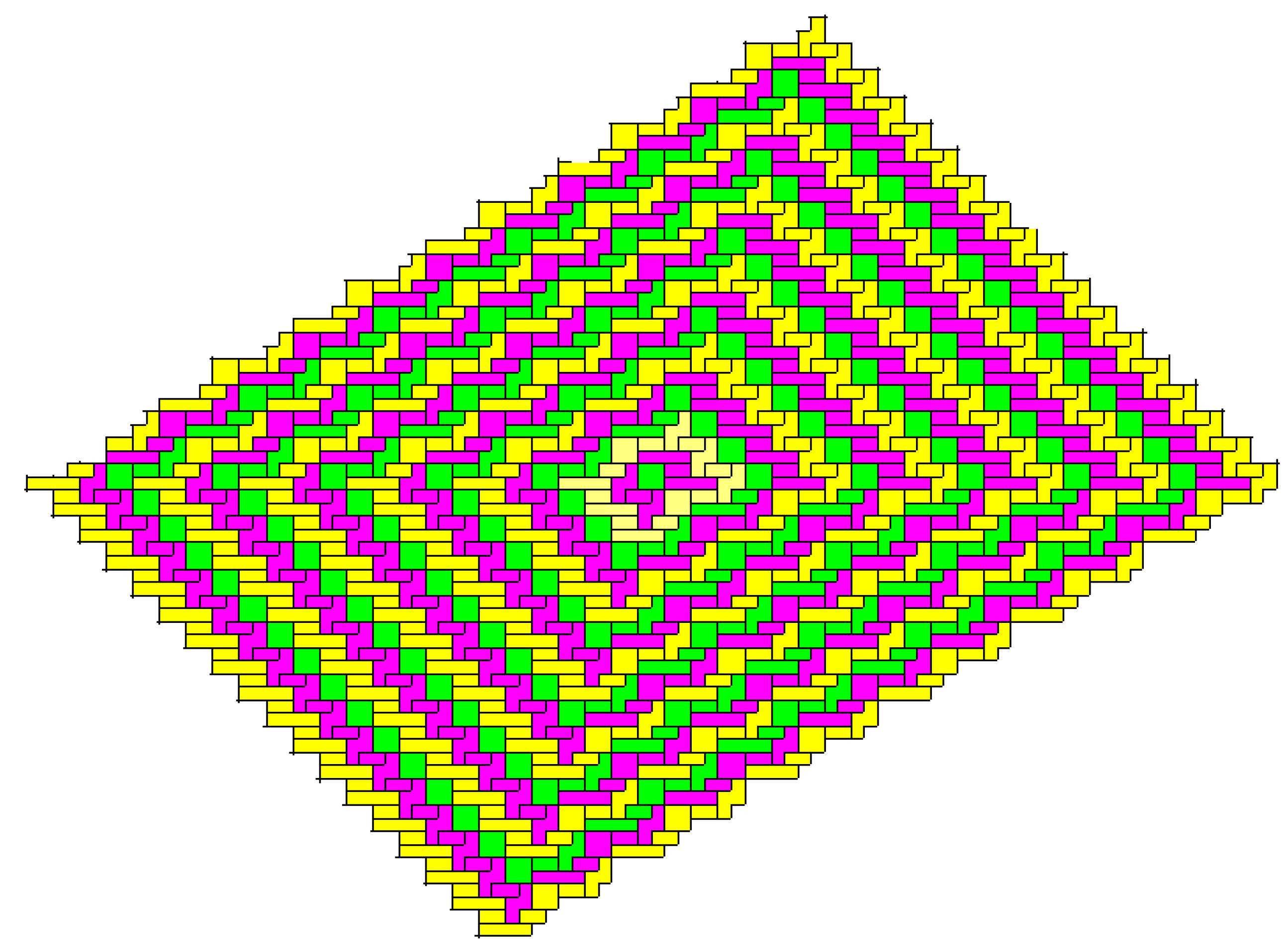
The packing space P84
1 8-color permutation operation g(13) = (0 13 7 14) (1 11 6 12) (2 10 5 9) (3 15 4 8) (16 30 23 31)(17 28 18 29) (19 27 20 26) (21 25 22 24) of the Cayley table of the Dirac matrices gives rise to partition (
Figure 19). The growth form of the partition structure is shown in
Figure 20.
Table 12.
Cayley table for the Dirac matrices group.
Table 12.
Cayley table for the Dirac matrices group.
| g[i] | [0] | [1] | [2] | [3] | [4] | [5] | [6] | [7] | [8] | [9] | [10] | 11] | [12] | [13] | [14] | [15] | [16] | [17] | [18] | [19] | [20] | [21] | [22] | [23] | [24] | [25] | [26] | [27] | [28] | [29] | [30] | [31] |
| [0] | [0] | [1] | [2] | [3] | [4] | [5] | [5] | [7] | [8] | [9] | [10] | [11] | [12] | [13] | [14] | [15] | [16] | [17] | [18] | [19] | [20] | [21] | [22] | [23] | [24] | [25] | [26] | [27] | [28] | [29] | [30] | [31] |
| [1] | [1] | [0] | [3] | [2] | [5] | [4] | [7] | [6] | [9] | [8] | [15] | [13] | [14] | [11] | [12] | [10] | [17] | [16] | [23] | [21] | [22] | [19] | [20] | [18] | [26] | [27] | [24] | [25] | [30] | [31] | [28] | [29] |
| [2] | [2] | [4] | [0] | [6] | [1] | [7] | [3] | [5] | [11] | [14] | [13] | [8] | [15] | [10] | [9] | [12] | [19] | [22] | [21] | [16] | [23] | [18] | [17] | [20] | [28] | [29] | [31] | [30] | [24] | [25] | [27] | [26] |
| [3] | [3] | [5] | [1] | [7] | [0] | [6] | [2] | [4] | [13] | [12] | [11] | [9] | [10] | [15] | [8] | [14] | [21] | [20] | [19] | [17] | [18] | [23] | [16] | [22] | [30] | [31] | [29] | [28] | [26] | [27] | [25] | [24] |
| [4] | [4] | [2] | [6] | [0] | [7] | [1] | [5] | [3] | [14] | [11] | [12] | [10] | [9] | [8] | [15] | [13] | [22] | [19] | [20] | [18] | [17] | [16] | [23] | [21] | [31] | [30] | [28] | [29] | [27] | [26] | [24] | [25] |
| [5] | [5] | [3] | [7] | [1] | [6] | [0] | [4] | [2] | [12] | [13] | [14] | [15] | [8] | [9] | [10] | [11] | [20] | [21] | [22] | [23] | [16] | [17] | [18] | [19] | [29] | [28] | [30] | [31] | [25] | [24] | [26] | [27] |
| [6] | [6] | [7] | [4] | [5] | [2] | [3] | [0] | [1] | [10] | [15] | [8] | [14] | [13] | [12] | [11] | [9] | [18] | [23] | [16] | [22] | [21] | [20] | [19] | [17] | [27] | [26] | [25] | [24] | [31] | [30] | [29] | [28] |
| [7] | [7] | [6] | [5] | [4] | [3] | [2] | [1] | [0] | [15] | [10] | [9] | [12] | [11] | [14] | [13] | [8] | [23] | [18] | [17] | [20] | [19] | [22] | [21] | [16] | [25] | [24] | [27] | [26] | [29] | [28] | [31] | [30] |
| [8] | [8] | [10] | [12] | [13] | [14] | [11] | [9] | [15] | [0] | [6] | [1] | [5] | [2] | [3] | [4] | [7] | [24] | [27] | [26] | [29] | [28] | [30] | [31] | [25] | [16] | [23] | [18] | [17] | [20] | [19] | [21] | [22] |
| [9] | [9] | [15] | [14] | [11] | [12] | [13] | [8] | [10] | [1] | [7] | [0] | [4] | [3] | [2] | [5] | [6] | [26] | [25] | [24] | [31] | [30] | [28] | [29] | [27] | [17] | [18] | [23] | [16] | [22] | [21] | [19] | [20] |
| [10] | [10] | [8] | [13] | [12] | [11] | [14] | [15] | [9] | [6] | [0] | [7] | [3] | [4] | [5] | [2] | [1] | [27] | [24] | [25] | [30] | [31] | [29] | [28] | [26] | [18] | [17] | [16] | [23] | [21] | [22] | [20] | [19] |
| [11] | [11] | [13] | [15] | [10] | [9] | [8] | [14] | [12] | [2] | [3] | [4] | [7] | [0] | [6] | [1] | [5] | [28] | [30] | [31] | [25] | [24] | [27] | [26] | [29] | [19] | [20] | [21] | [22] | [23] | [16] | [18] | [17] |
| [12] | [12] | [14] | [8] | [9] | [10] | [15] | [13] | [11] | [5] | [4] | [3] | [0] | [7] | [1] | [6] | [2] | [29] | [31] | [30] | [24] | [25] | [26] | [27] | [28] | [20] | [19] | [22] | [21] | [16] | [23] | [17] | [18] |
| [13] | [13] | [11] | [10] | [15] | [8] | [9] | [12] | [14] | [3] | [2] | [5] | [6] | [1] | [7] | [0] | [4] | [30] | [28] | [29] | [27] | [26] | [25] | [24] | [31] | [21] | [22] | [19] | [20] | [18] | [17] | [23] | [16] |
| [14] | [14] | [12] | [9] | [8] | [15] | [10] | [11] | [13] | [4] | [5] | [2] | [1] | [6] | [0] | [7] | [3] | [31] | [29] | [28] | [26] | [27] | [24] | [25] | [30] | [22] | [21] | [20] | [19] | [17] | [18] | [16] | [23] |
| [15] | [15] | [9] | [11] | [14] | [13] | [12] | [10] | [8] | [7] | [1] | [6] | [2] | [5] | [4] | [3] | [0] | [25] | [26] | [27] | [28] | [29] | [31] | [30] | [24] | [23] | [16] | [17] | [18] | [19] | [20] | [22] | [21] |
| [16] | [16] | [18] | [20] | [21] | [22] | [19] | [17] | [23] | [25] | [26] | [27] | [28] | [29] | [31] | [30] | [24] | [0] | [6] | [1] | [5] | [2] | [3] | [4] | [7] | [15] | [8] | [9] | [10] | [11] | [12] | [14] | [13] |
| [17] | [17] | [23] | [22] | [19] | [20] | [21] | [16] | [18] | [27] | [24] | [25] | [30] | [31] | [29] | [28] | [26] | [1] | [7] | [0] | [4] | [3] | [2] | [5] | [6] | [10] | [9] | [8] | [15] | [13] | [14] | [12] | [11] |
| [18] | [18] | [16] | [21] | [20] | [19] | [22] | [23] | [17] | [26] | [25] | [24] | [31] | [30] | [28] | [29] | [27] | [6] | [0] | [7] | [3] | [4] | [5] | [2] | [1] | [9] | [10] | [15] | [8] | [14] | [13] | [11] | [12] |
| [19] | [19] | [21] | [23] | [18] | [17] | [16] | [22] | [20] | [29] | [31] | [30] | [24] | [25] | [26] | [27] | [28] | [2] | [3] | [4] | [7] | [0] | [6] | [1] | [5] | [12] | [11] | [14] | [13] | [8] | [15] | [9] | [10] |
| [20] | [20] | [22] | [16] | [17] | [18] | [23] | [21] | [19] | [28] | [30] | [31] | [25] | [24] | [27] | [26] | [29] | [5] | [4] | [3] | [0] | [7] | [1] | [6] | [2] | [11] | [12] | [13] | [14] | [15] | [8] | [10] | [9] |
| [21] | [21] | [19] | [18] | [23] | [16] | [17] | [20] | [22] | [31] | [29] | [28] | [26] | [27] | [24] | [25] | [30] | [3] | [2] | [5] | [6] | [1] | [7] | [0] | [4] | [14] | [13] | [12] | [11] | [9] | [10] | [8] | [15] |
| [22] | [22] | [20] | [17] | [16] | [23] | [18] | [19] | [21] | [30] | [28] | [29] | [27] | [26] | [25] | [24] | [31] | [4] | [5] | [2] | [1] | [6] | [0] | [7] | [3] | [13] | [14] | [11] | [12] | [10] | [9] | [15] | [8] |
| [23] | [23] | [17] | [19] | [22] | [21] | [20] | [18] | [16] | [24] | [27] | [26] | [29] | [28] | [30] | [31] | [25] | [7] | [1] | [6] | [2] | [5] | [4] | [3] | [0] | [8] | [15] | [10] | [9] | [12] | [11] | [13] | [14] |
| [24] | [24] | [26] | [28] | [30] | [31] | [29] | [27] | [25] | [23] | [18] | [17] | [20] | [19] | [22] | [21] | [16] | [8] | [9] | [10] | [11] | [12] | [13] | [14] | [15] | [7] | [0] | [6] | [1] | [5] | [2] | [4] | [3] |
| [25] | [25] | [27] | [29] | [31] | [30] | [28] | [26] | [24] | [16] | [17] | [18] | [19] | [20] | [21] | [22] | [23] | [15] | [10] | [9] | [12] | [11] | [14] | [13] | [8] | [0] | [7] | [1] | [6] | [2] | [5] | [3] | [4] |
| [26] | [26] | [24] | [30] | [28] | [29] | [31] | [25] | [27] | [18] | [23] | [16] | [22] | [21] | [20] | [19] | [17] | [9] | [8] | [15] | [13] | [14] | [11] | [12] | [10] | [6] | [1] | [7] | [0] | [4] | [3] | [5] | [2] |
| [27] | [27] | [25] | [31] | [29] | [28] | [30] | [24] | [26] | [17] | [16] | [23] | [21] | [22] | [19] | [20] | [18] | [10] | [15] | [8] | [14] | [13] | [12] | [11] | [9] | [1] | [6] | [0] | [7] | [3] | [4] | [2] | [5] |
| [28] | [28] | [31] | [24] | [27] | [26] | [25] | [30] | [29] | [20] | [21] | [22] | [23] | [16] | [17] | [18] | [19] | [11] | [14] | [13] | [8] | [15] | [10] | [9] | [12] | [5] | [2] | [3] | [4] | [7] | [0] | [1] | [6] |
| [29] | [29] | [30] | [25] | [26] | [27] | [24] | [31] | [28] | [19] | [22] | [21] | [16] | [23] | [18] | [17] | [20] | [12] | [13] | [14] | [15] | [8] | [9] | [10] | [11] | [2] | [5] | [4] | [3] | [0] | [7] | [6] | [1] |
| [30] | [30] | [29] | [26] | [25] | [24] | [27] | [28] | [31] | [22] | [19] | [20] | [18] | [17] | [16] | [23] | [21] | [13] | [12] | [11] | [9] | [10] | [15] | [8] | [14] | [4] | [3] | [2] | [5] | [6] | [1] | [0] | [7] |
| [31] | [31] | [28] | [27] | [24] | [25] | [26] | [29] | [30] | [21] | [20] | [19] | [17] | [18] | [23] | [16] | [22] | [14] | [11] | [12] | [10] | [9] | [8] | [15] | [13] | [3] | [4] | [5] | [2] | [1] | [6] | [7] | [0] |
Figure 19.
Tiling PS P84
1 by permutation operation g (13) (
Table 12) of the Dirac matrices group.
Figure 19.
Tiling PS P84
1 by permutation operation g (13) (
Table 12) of the Dirac matrices group.
Figure 20.
Octagon of the growth structure partition (
Figure 19) on the PS P84
1.
Figure 20.
Octagon of the growth structure partition (
Figure 19) on the PS P84
1.
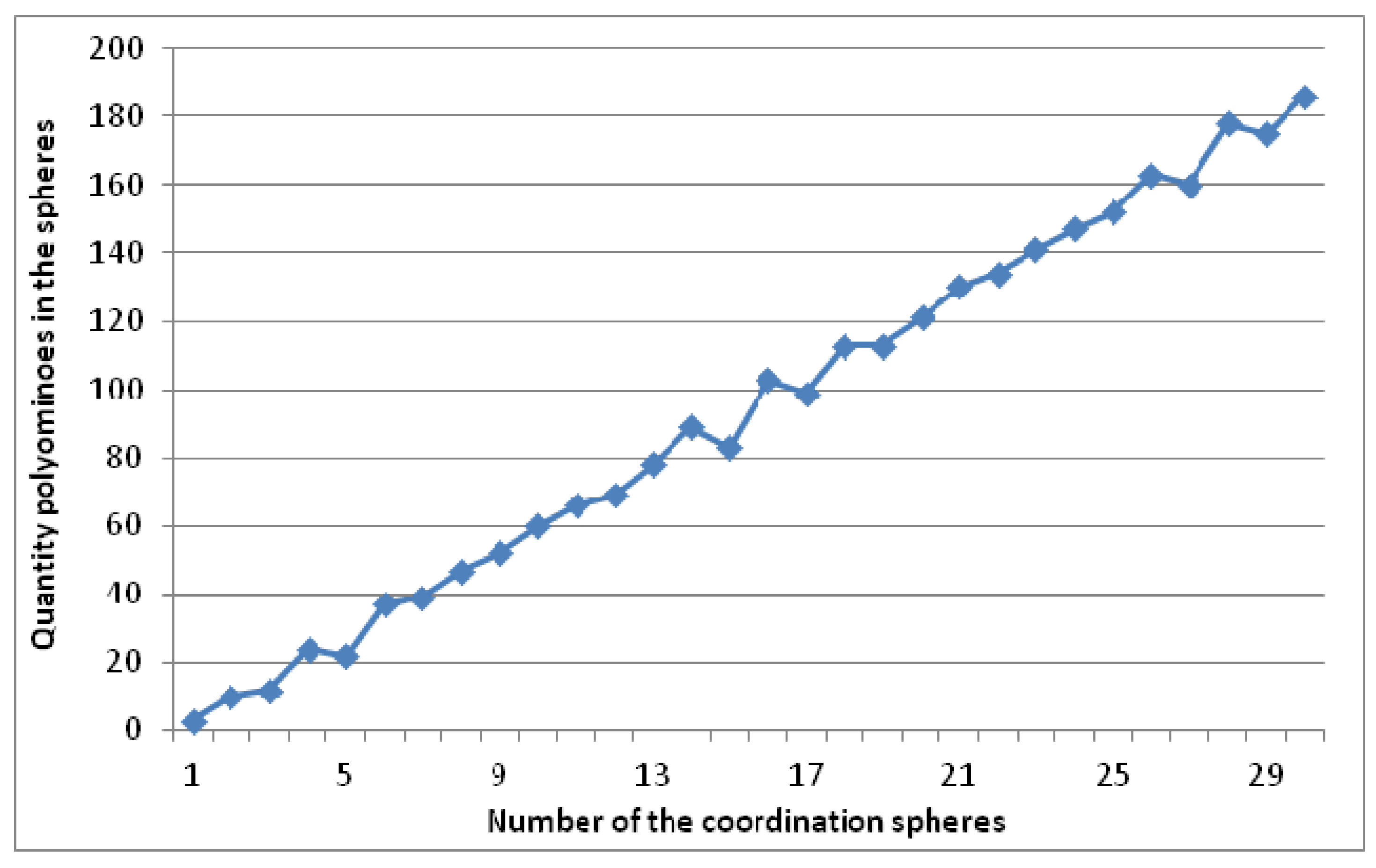
The numerical sequence of filling the coordination spheres of the growing figure in the PS 84
1 depends on the choice of “seed polyomino”, but the limiting form of the growth, which is the choice of the different growth beginning, is always the same, as presented in [
18]. The only linear dependence of polyominoes quantity in the layer is on the layer number “on average” (
Figure 21), which is uncommon for two-dimensional partitions [
16].
In this article, we will not analyze the use of information received on the Pauli and Dirac matrices and the structure of the groups, although there is a connection of physical theory with the design obtained by partition of packing spaces. A search for the connection can be conducted in two ways: First, to identify what group properties determine the structure of the partition, and, second, to determine if there is a real structure, which is subordinate to discrete representation of these groups.
To answer the arising questions, it is necessary to consider the transition procedure from the real structure to its discrete model based on permutation operations.
Figure 21.
Coordination (magic) numbers of growth structure (
Figure 19).
Figure 21.
Coordination (magic) numbers of growth structure (
Figure 19).
3.6. An Example of a Real Structure with Non-Crystallographic Permutation Group Symmetry
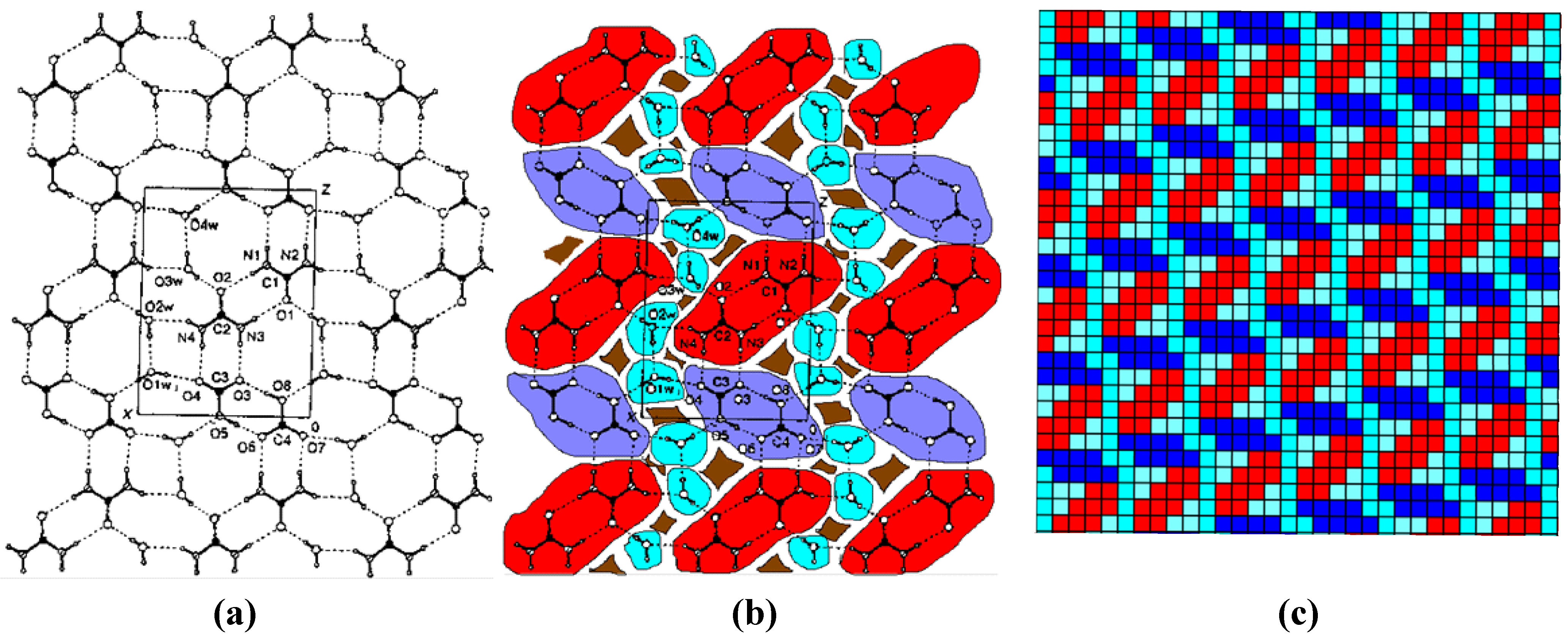
For the partition of three-dimensional structures, you can use the methodology for constructing molecular domains of Voronoi–Dirichlet by means of Fisher and Koch (see for example, reference [
25]). However, as the analysis of three-dimensional partitions of a periodic lattice is hard to perceive, we choose the real structure of [(C
2H
5)
4N
+]
2·C
4O
42−·2(C
2H
5)
4N + HCO
3−∙4(NH
2)
2CO∙6H
2O [
27], based on a molecular layer (
Figure 22). We use a qualitative approach: select the layer of the two types of dimer: 2(HCO
3)
−, 2CO(NH
2)
2 and two pairs of water molecules per unit cell, bound by hydrogen bonds. The result is a three-colored partition “map” into non-overlapping substructures (
Figure 22b).
Figure 22.
The molecular layer (a) in the structure of the compound [(C2H5)4N+]2·C4O42−·2(C2H5)4N + HCO3−∙4(NH2)2CO∙6H2O, “map” of its partition; (b) into disjoint regions and (c) the discrete layer structure model.
Figure 22.
The molecular layer (a) in the structure of the compound [(C2H5)4N+]2·C4O42−·2(C2H5)4N + HCO3−∙4(NH2)2CO∙6H2O, “map” of its partition; (b) into disjoint regions and (c) the discrete layer structure model.
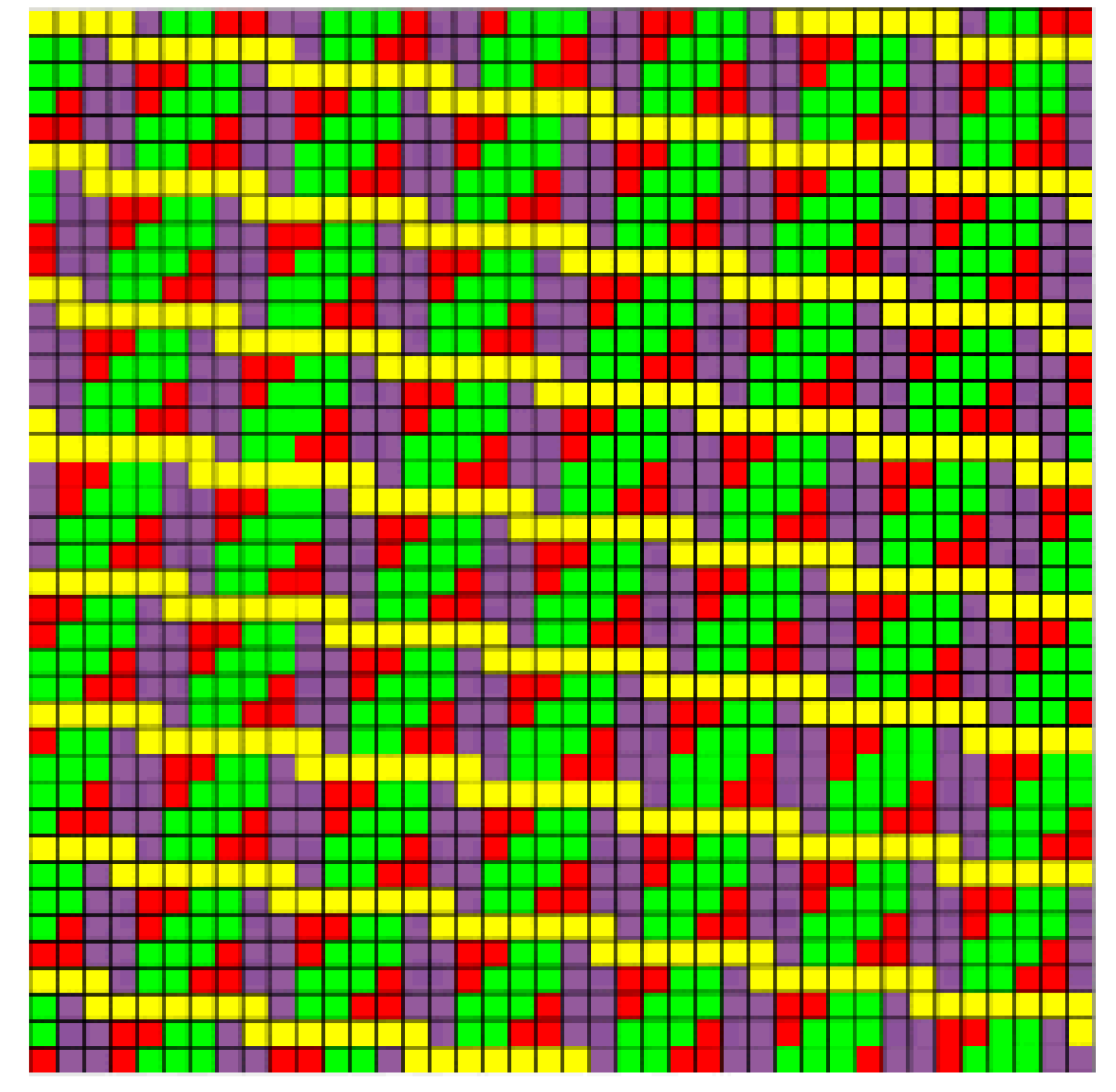
Without changing the coordination environment of each region, a polyomino-like presentation of this structure’s layer (
Figure 22c) is obtained for the packing space P31 1
6. The sizes of cells are selected in such way that the order of the cell of packing space is a prime number
N = 31. The number of independent types of lattices in this case is minimal, which is important when iterating the options in the prediction structures task. The image of the PS P31
6 structure, rotated to locate the yellow-red layer consisting of water molecules horizontally, is presented in
Figure 23. The form of layered structure growth is presented in [
16].
Figure 23.
A discrete model of the structure layer [
27] in PS P31 1
6.
Figure 23.
A discrete model of the structure layer [
27] in PS P31 1
6.
In this example, the formed four-colored operation of permutation is written as follows:
G(1) = (1 2 3 28 10 11 5 8 14 15 9 18 6 12 17 16 22 23 25 13 19 27 21 24 7 26 20 4 29 30 0)
= (0 1 2 3 28 29 30) (4 10 9 15 16 22 21 27 ) (5 11 18 25 26 20 19 13 12 6) (7 8 14 17 23 24).
In this article, we do not give a Cayley matrix of the cyclic group (G (1))m, which has an order greater than 2N. In terms of group properties, it is interesting that when the order of m = p, where p is a prime number >10, the structure is invariant. Rearrangements occur within the number of cycles, and we use this fact to calculate the statistical probability and statistical entropy:
WT = 31!/6!7!8!10! = 1013; σ = lnWT = 13ln10 = 29,9.
The formula of Boltzmann’s entropy of the structure is S = klnWT = 41.3 × 10⁻²³ (J/K).
In other orders of m, the number of cycles (color set in the PS P31 16 partition) changes, as well as their structure and entropy.
Keeping the original structure unchanged, that is, without changing the operation G(1), we consider gradual deformation of the structure when there is a transition from one packing space with
N = 31k to another, the number of which, as for the primes, is equal to
N + 1 = 32 (
Figure 24).
The first and last PS P31 1
0 and P31 1
30 are not completely presented in
Figure 24. It is easily observed from the slope of the layers in the partition that the deformation transformations of the lattice shift result in similar pairs of partitions associated with each other as “left” and “right” forms. These phase structures are obtained by a mirror image.
Figure 24.
Discrete deformation transformations of the layer structure [
27] in the PS P31 1
6 partition model (in
Figure 22). The frames mark “left” and “right” forms of the structure.
Figure 24.
Discrete deformation transformations of the layer structure [
27] in the PS P31 1
6 partition model (in
Figure 22). The frames mark “left” and “right” forms of the structure.
4. Brief Summary
1. Discrete modeling of tilings and packages, as well as the introduction of packing space, allow us to make space partitions into any fragments in a periodic lattice. In this article, we present for the first time the method of the exhaustive search option sublattices with index N based on the analysis of irreducible representations of a mathematical group of permutations of the N2 elements.
2. The developed partition algorithms and software packages (not covered in this article) make it possible to partition and predict the structure of molecular compounds using the criterion of partition presented in this article. The criterion answers the question: What polyomino or policube may be a fundamental area in a periodic lattice?
3. Application of the layer growth model and growth of the graph in the space partition allows us to calculate structures of real crystalline nuclei and nanoclusters model. Algorithms and programs for the calculations in the article are not presented as they were released previously. The results of calculating the polyhedra growth of structures formed by partitioning of the space with the use of groups of permutations are considered for the first time in this work, and the figures of growth can be one of the characteristics of group 4. Application of finite groups of permutations to the packing space determines space partition into policubes (polyominoes), and forms a structure. This allows you to expand the capabilities of the description of symmetry of periodic structures and is not limited to 230 space groups.
5. Any finite groups, expressed through a group of permutations and applied to the packing space, are structurally visualized.
6. The totality of packaging spaces of the same order N characterizes the discrete deformation transformation of the corresponding periodic structure.
7. Application of the methodology, based on the PS formalism, will contribute to the transfer to the numeric “language”, and it is essential that a significant amount of information about the structures that do work be obtained with computers that operate only with numbers.


