Supersymmetric Sigma Model Geometry

Abstract
: This is a review of how sigma models formulated in Superspace have become important tools for understanding geometry. Topics included are: The (hyper)kähler reduction; projective superspace; the generalized Legendre construction; generalized Kähler geometry and constructions of hyperkähler metrics on Hermitian symmetric spaces.Classification: PACS 11.30.Pb
Classification: MSC 53Z05
1. Introduction
Sigma models take their name from a phenomenological model of beta decay introduced more than fifty years ago by Gell-Mann and Lévy [1]. It contains pions and a new scalar meson that they called sigma. A generalization of this model is what is nowadays meant by a sigma model. It will be described in detail below.
Non-linear sigma models arise in a surprising number of different contexts. Examples are effective field theories (coupled to gauge fields), the scalar sector of supergravity theories etc. Not the least concern to modern high energy theory is the fact that the string action has the form of a sigma model coupled to two dimensional gravity that the compactified dimensions carry the target space geometry dictated by supersymmetry.
The close relation between supersymmetric sigma models and complex geometry was first observed more than thirty years ago in [2] where the target space of N = 1 models in four dimensions is shown to carry Kähler geometry. For N = 2 models in four dimensions the target space geometry was subsequently shown to be hyperkähler in [3]. This latter fact was extensively exploited in a N = 1 superspace formulation of these models in [4], where two new constructions were presented; the Legendre transform construction and the hyperkähler quotient construction. The latter reduction was developed and given a more mathematically stringent formulation in [5] where we also elaborated on a manifest N = 2 formulation, originally introduced in [6] based on observations in [7].
A N = 2 superspace formulation of the N = 2 four dimensional sigma model is obviously desirable, since it will automatically lead to hyperkähler geometry on the target space. The N = 2 Projective Superspace which makes this possible grew out of the development mentioned last in the preceding paragraph. Over the years it has been developed and refined in, e.g., [6,7,8,9,10,11,12,13,14,15,16,17,18,19]. In this article we report on some of that development along with some more recent development, such as projective superspace for supergravity [20,21,22,23,24,25], and applications such as the construction of certain classes of hyperkähler metrics [26,27,28].
The target space geometry depends on the number of supersymmetries as well as on the dimension of the domain. There are a number of features peculiar to sigma models with a two dimensional domain (2D sigma models). Here the target space geometry can be torsionful and generalizes the Kähler and hyperkähler geometries. This has been exploited to give new and interesting results in generalized geometry [29,30,31,32,33,34,35,36,37,38,39,40,41].
Outside the scope of this report lies, e.g., Kähler geometries with additional structure, such as special geometry relevant for four dimensional N = 2 sigma models, (see, e.g., [42]).
All our presentations will concern the classical theory. We shall not discuss the interesting and important question of quantization.
2. Sigma Models
A non-linear sigma model is a theory of maps from a (super) manifold ∑(d, N) to a target space (we shall mostly avoid global issues and assume that all of T can be covered by such maps in patches) T:

Denoting the coordinates on ∑(d, N) by z = (ξ,θ), the maps are derived by extremizing an action

The actual form of the action depends on the bosonic and fermionic dimensions dB, dF of Σ. We have temporarily included a boundary term, which is sometimes needed for open models to have all the symmetries of the bulk-theory [43,44,45], or when there are fields living only on the boundary coupling to the bulk fields as is the well known case for (stacks of) D-branes. For a discussion of the latter in a sigma model context, see [46]. Expanding the superfield as Φ(ξ, θ) = X + θΨ+ …, where X(ξ) and Ψ(ξ) are bosonic and fermionic fields over the even part of Σ (coordinatized by ξ), the action Equation (2) becomes

where d = dB is the bosonic dimension of Σ and we have rescaled the X’s to make them dimensionless, thus introducing the mass-scale μ.
Let us make a few general comments about the action Equation (3), mostly quoted from Hull [47]:
1. The mass-scale μ shows that the model typically will be non-renormalizable for d ≥ 3 but renormalizable and classically conformally invariant in d = 2.
2. We have not included a potential for X and thus excluded Landau–Ginsburg models.
3. There is also the possibility to include a Wess–Zumino term. We shall return to this when discussing d = 2.
4. From a quantum mechanical point of view it is useful to think of Gμv(X) as an infinite number of coupling constants:
![Symmetry 04 00474 i004]()
5. Classically, it is more rewarding to emphasize the geometry and think of Gμv(X) as a metric on the target space T. This is the aspect we shall be mainly concerned with.
6. The invariance of the action S under Diff(T),
field-redefinitions from the point of view of the field theory on Σ), implies that the sigma model is defined by an equivalence class of metrics. N.B. This is not a symmetry of the model since the “coupling constants” also transform. It is an important property, however. Classically it means that the model is extendable beyond a single patch in T, and quantum mechanically it is needed for the effective action to be well defined.![Symmetry 04 00474 i005]()


That the geometry of the target space T is inherently related to the sigma model is clear already from the preceding comments. Further, the maps extremizing S satisfy

where  , the operator ∇ is the Levi-Civita connection for Gμv and we have ignored the fermions. This is the pull-back of the covariant Laplacian on T to Σ and hence the maps are sometimes called harmonic maps.
The geometric structure that has emerged from the bosonic part shows that the target space geometry must be Riemannian (by which we mean that it comes equipped with a metric and corresponding Levi-Civita connection). Further restrictions arise from supersymmetry.
3. Supersymmetry
This section provides a very brief summary of some aspects of supersymmetry. For a thorough introduction the reader should consult a textbook, e.g., [48,49,50].
At the level of algebra, supersymmetry is an extension of the d-dimensional Poincaré-algebra to include anticommuting charges Q. The form of the algebra depends on d. In dB = 4 the additional (anti-)commutators satisfy

Here α, β,.. are four dimensional spinor indices, Υi are Dirac gamma matrices, C is the (electric) charge conjugation matrix and the charges Qa are spinors that satisfy a Majorana reality condition and transform under some internal symmetry group G ⊂ O(N) (corresponding to the index a). The generators of the graded Poincaré-algebra are thus the Lorentz-generators M, the generators of translations P and the supersymmetry generators Q. In addition, for non-trivial G, there are central charge generators Z and Y that commute with all the others.
Representations of supersymmetry are most economically collected into superfields Φ(ξ, θ), where θa are Grassmann valued spinorial “coordinates” to which one can attach various amounts of importance. We may think of them as a book-keeping device, much as collecting components into a column-vector. But thinking about (ξ, θ) as coordinates on a supermanifold M(d, N)[51,52] and investigating the geometry of this space has proven a very fruitful way of generating interesting results.
The index a on θa is the same as that on Qa and thus corresponds to the number N of supersymmetries. Let us consider the case N = 1, dB = 4, which implies Z = Y = 0. In a Weyl-representation of the spinors and with the usual identification of the translation generator as a differential operator  , the algebra Equation (7) becomes

Introducing Berezin integration/derivation [53],  , the supercharges Q may also be represented (in one of several possible representations) as differential operators acting on superfields:

Apart from the various representations alluded to above (chiral, antichiral and vector in four dimensions [48]) there are two basic ways that supercharges can act on superfields, corresponding to left and right group action. This means that, given Equation (9), there is a second pair of differential operators

which also generate the algebra Equation (8) and that anticommute with the Q’s:

Often the supersymmetry algebra is given only in terms of the D’s. From a geometrical point of view, these are covariant derivatives in superspace and may be used to impose invariant conditions on superfields.
In general, covariant derivatives ∇A in a curved superspace space satisfy
where the left hand side contains a graded commutator TABC is the torsion tensor and  the curvature with
  the generators of the structure group. The indices Aetc. run over both bosonic and fermionic indices. Comparision to Equation (11), with
  , shows that even “flat” (
  ) superspace has torsion.
In four dimensions the D’s may be used to find the smallest superfield representation. Such a chiral superfield ϕ and its complex conjugate antichiral field  are required to satisfy

The Minkowski-field content of this may be read off from the θ-expansion. However, this expansion depends on the particular representation of the D’s and Q’. For this reason it is preferable to define the components in the following representation independent form:

where a vertical bar denotes “the θ-independent part of”. In a chiral representation where  the θ-expansion of a chiral field reads

but its complex conjugate involves a θ dependent shift in ξ and looks more complicated.
A dimensional analysis shows that if X is a physical scalar, χ is a physical spinor and F has to be a non-propagating (auxiliary) field. This is the smallest multiplet that contains a scalar, and thus suitable for constructing a supersymmetric extension of the bosonic sigma models we looked at so far. (All other superfields will either be equivalent to (anti) chiral ones or contain additional bosonic fields of higher spin.) Denoting a collection of chiral fields by ϕ = (ϕμ), the most general action we can write down

reduces to the bosonic integral

The most direct way to perform the reduction is to write

and then to use Equation (13) when acting with the covariant spinor derivatives. Note that K in Equation (16) is only defined up to a term  due to the chirality conditions as in Equation (13).
We immediately learn additional things about the geometry of the target space T:
1. It must be even-dimensional.
2. The metric is Hermitian with respect to the canonical complex structure
for which X and![Symmetry 04 00474 i029]()
![Symmetry 04 00474 i030]() are canonical coordinates.
are canonical coordinates.3. The metric has a potential
![Symmetry 04 00474 i031]() . In fact, the geometry is Kähler and the ambiguity in the Lagrangian in Equation (16) is known as a Kähler gauge transformation.
. In fact, the geometry is Kähler and the ambiguity in the Lagrangian in Equation (16) is known as a Kähler gauge transformation.


4. Complex Geometry I
Let us interrupt the description of sigma models to recapitulate the essentials of Kähler geometry.
Consider (M, G, J) where G is a metric on the manifold M and J is an almost complex structure, i.e., an endomorphism(A (1,1) tensor Jvμ.)  such that J2 = −1 (only possible if M is even dimensional). This is an almost Hermitian space if (as matrices)

Construct the projection operators

If the vectors π±V in T are in involution, i.e., if

which implies that the Nijenhuis torsion vanishes,

then the distributions defined by π± are integrable and J is called a complex structure and G Hermitian. To evaluate the expression in Equation (22) in index notation, think of π∓ as matrices acting on the components of the Lie bracket between the vectors π±V and π±U. This leads to the following expression corresponding to Equation (23):

The fundamental two-form ω defined by J and G is

If it is closed for a Hermitian complex space, then the metric has a Kähler potential

and the geometry is Kähler.
An equivalent characterization is as an almost Hermitian manifold with

where ∇ is the Levi-Civita connection.
We shall also need the notion of hyperkähler geometry. Briefly, for such a geometry there exists an SU(2)-worth of complex structures labeled by A ∈ {1,2,3}

with respect to all of which the metric is Hermitian

5. Sigma Model Geometry
We have already seen how N = 1 (one supersymmetry) in d = 4 requires the target space geometry to be Kähler. To investigate how the geometry gets further restricted for N = 2, there are various options: (i) Discuss the problem entirely in components (no supersymmetry manifest); (ii) Introduce projective (or harmonic) superspace and write models with manifest N = 2 symmetry; (iii) Add a non-manifest supersymmetry to the model already described and work out the consequences. The last option requires the least new machinery, so we first follow this. The question is thus under what conditions

can support an additional supersymmetry. The most general ansatz for such a symmetry is

One finds closure of the additional supersymmetry algebra (on-shell) and invariance of the action provided that the target space geometry is hyperkähler with the non-manifest complex structures formed from Ω [54]:

Further, the parameter superfield ε obeys

It contains the parameter for central charge transformations along with the supersymmetry parameters.
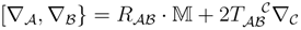
The full table of geometries for supersymmetric non-linear sigma models without Wess–Zumino term reads
(Odd dimensions have the same structure as the even dimension lower.) When we specialize to two or six dimensions, we have the additional possibility of having independent left and right supersymmetries; the N = (p, q) supersymmetries of Hull and Witten [55]. We shall return to this possibility when we discuss d = 2, but now we turn to the question of how to gauge isometries on Kähler and hyperkähler manifolds.
6. Gauging Isometries and the HK Reduction
This section is to a large extent a review of [54,5].
6.1. Gauging Isometries of Bosonic Sigma Models
The table in the previous section describing the target-space geometry shows that constructing, e.g., new N = 2, d = 4 nonlinear sigma models is tantamount to finding new hyper-kähler geometries. A systematic method for doing this involves isometries of the target space, which we now discuss.
Consider again the bosonic action

As noted in Section 2, a target space diffeomorphism leaves this action invariant and corresponds to a field redefinition. As also pointed out, this is not a symmetry of the field theory. A symmetry of the field theory involves a transformation of ϕ only;

where Lλk denotes the Lie derivative along the vector λk. Under such a transformation the action varies as

The transformation thus gives an invariance of the action if

i.e., if the transformation is an isometry and hence if the kAμ’s are Killing-vectors.
We take the kA’s to generate a Lie algebra g

with

In what follows, we assume that g can be exponentiated to a group G.
One way to construct a new sigma model from one which has isometries is to gauge the isometries and then find a gauge connection that extremizes the action [54]. The new sigma model will be a quotient of the original one. Briefly, this goes as follows:
The isometries generated by kA are gauged introducing a gauge field AiA using minimal coupling,

in the action Equation (34):

This action is now locally invariant under the symmetries defined by the algebra Equation (38). Note that there is no kinetic term for the gauge-field. Extremizing Equation (41) with respect to AiA singles out a particular gauge-field:
where
In terms of this particular connection, the action Equation (41) now reads
where indices have been lowered using the metric G. Since  in the action Equation (44 ), this is a new sigma model defined on the space of orbits of the group G, i.e., on the quotient space T/G. The metric on this space is
  .
.
To apply this construction to Kähler manifolds, or equivalently, supersymmetric models, in such a way as to preserve the Kähler properties, more restrictions are required. First, the isometries we need to gauge are holomorphic and the gauge group we have to consider is the complexification of the group relevant to the bosonic part.
6.2. Holomorphic Isometries
A holomorphic isometry on a Kähler manifold satisfies

where J is the complex structure and ω is the Kähler two-form defined in Equation (25). The fact that a Kähler manifold is symplectic makes it possible to consider the moment map for the Hamiltonian vector field λk. The corresponding Hamiltonian function μλk is defined by

In holomorphic coordinates  where
where  , this reads

From these relations it is clear why μλk is sometimes referred to as a Killing potential. Now μ defines a map from the target space of the sigma model into the dual of the Lie-algebra generated by kA:

where μA is the basis for *g that corresponds to the basis kA for g. When the action of the Hamiltonian field can be made to agree with the natural action of the group G on T and on *g, the μA’s are called moment maps (We use to the (US) East cost nomenclature as opposed to the West coast “momentum map”.) This is the case when μλk is equivariant, i.e., when

where the equivalence refers to holomorphic isometries.
The Kähler metric is the Hessian of the Kähler potential K. As mentioned in Section 3, this leaves an ambiguity in the potential; it is only defined up to the sum of a holomorphic and an antiholomorphic term.

An isometry thus only has to preserve K up to such terms:

For a holomorphic isometry  this implies for the projection

(Recall that  and
and  , so that
  +hol. and
  +antihol. )
6.3. Gauging Isometries of Supersymmetric Sigma Models
Due to the chiral nature of superspace, the isometries act through the complexification of the isometry group G. Explicitly, the parameter λgets replaced by superfield parameters  and
and  , while the bosonic gauge field AiA becomes one of the components of a real superfield VA. (This is the last occurrence of i as a world volume index. Below i, j,… denote gauge indies.) In the simplest case of isotropy, kAi(ϕ) = (TA)jiϕj, the coupling to the chiral fields in the sigma model is

At the same time, a gauge transformation with (chiral) parameter acts on the chiral and antichiral fields as

The relation Equation (53) can thus be interpreted as a gauge transformation of with parameter iV. For general isometries a gauge transformation with parameter iV is

and this is the form we need to use when defining  . The coupling is thus

Under a global isometry transformation, according to Equation (51), there may arise terms such as

whose vanishing ensures the invariance. This is no-longer true in the local case where the corresponding term

will not vanish in general. The remedy is to introduce auxiliary coordinates  and assign transformations to them that make the modified Kähler potential
  invariant (rather than invariant up to (anti) holomorphic terms):

The action involving may now be gauged using the prescription Equation (56) and takes the form (dropping the irrelevant  term after gauging)

where

Using the definition of  and the relation to the moment maps (see Equation (52) and below), we rewrite this as

A more geometric form of the gauged Lagrangian is

where we recall that

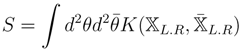
The form of the action that follows from Equation (63) directly leads to the symplectic quotient as applied to a Kähler manifold [56]: Eliminating VA results in

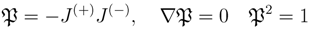
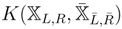
The Kähler quotient is illustrated in the following picture, taken from [5] (with permission from the publisher Springer Verlag) :
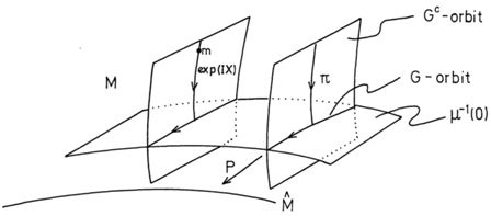
The isometry group G acts on μ−1(0) and produces the quotient  . The same space is obtained if one considers the extension of μ−1(0) by exp(JX) and takes the quotient by the complexified group GC.
If we start from a hyperkähler manifold with triholomorphic isometries, there will also be complex moment maps corresponding to the two non-canonical complex structures

In addition to Equation (65), we will then have the conditions

defining holomorphic subspaces. This hyperkähler quotient prescription [4,5] gives a new hyperkähler space from an old one. The N = 2 sigma model action that encodes this (in d = 4, N = 1 language) reads

where  is defined in Equation (61) and
  is the N = 2 vector (gauge) multiplet. The latter consists of a chiral superfield S and its complex conjugate
  in addition to V.
7. Two Dimensional Models and Generalized Kähler Geometry
The quotient constructions just discussed are limited to backgrounds with only a metric present. Recently extensions of such geometries to include also an antisymmetric B-field have led to a number of new results in d = 2 which are expected to contribute to new quotients involving such geometries.
Two (bosonic) dimensional domains Σ are interesting in that they support sigma models with independent left and right supersymmetries. Such (p, q) models were introduced by Hull and Witten in [55], and also have analogues in d = 6. There is a wealth of results on the target-space geometry for (p, q)-models. The geometry is typically a generalization of Kähler geometry with vector potential for the metric instead of a scalar potential etc. See, e.g., [57,58]. Here we first focus on (1,1) and (2,2) models in d = 2.
The (1,1) supersymmetry algebra is

where + and − are spinor indices and  are light-cone coordinates in d = 2 Minkowski space.
A general sigma model written in terms of real N = (1,1) superfields ϕ is

where the metric G and B-field have been collected into

Here N = (1,1) supersymmetry is manifest by construction and we shall see that additional non-manifest ones will again restrict the target space geometry. In fact, the geometry is already modified due to the presence of the B-field. The field-equations now read

where

is the sum of the Levi-Civita connection and a torsion-term formed from the field-strength for the B-field (The anti-symmetrization does not include a combinatorial factor):

Only when H = 0 do we recover the non-torsionful Riemann geometry. The full picture is given in the following table:

| Supersymmetry | (0,0) or (1,1) | (2,2) | (2,2) | (4,4) | (4,4) |
|---|---|---|---|---|---|
| Background | G,B | G | G,B | G | G,B |
| Geometry | Riemannian | Kähler | bi-Hermitian | hyperkähler | bihypercomplex |
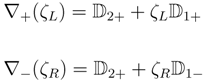
We first look at the Gates–Hull–Roček (GHR) bi-Hermitian geometry, or Generalized Kähler geometry as is its modern guise. Starting from the N = (1,1) action Equation (7), one can ask for additional, non-manifest supersymmetries. By dimensional arguments, such a symmetry must act on the superfields as

where (±) correspond to left or right symmetries. It was shown by GHR in [7] that invariance of the action Equation (7) and closure of the algebra require that J(±) are complex structures that are covariantly constant with respect to the torsionful connections

and that the metric is Hermitian with respect to both these complex structures

In addition, the B-field field-strength (torsion) must obey

where the chirality assignment refers to both complex structures. Here we have introduced  , where the last equality holds in canonical coordinates, the two-forms are ω(±) ≡ GJ(±) as tensors and
  . When J(+) = ±J(−) this geometry reduces to Kähler geometry.
Gualtieri gives a nice interpretation of the full bi-Hermitian geometry in the context of Generalized Complex Geometry [59] and calls it Generalized Kähler Geometry [60], which we now briefly describe.
8. Complex Geometry II
The definition of Generalized Complex Geometry (GCG) parallels that of complex geometry but is based on the sum of the tangent and cotangent bundle instead of just the tangent bundle. Hence we consider a section J of End(T⊕T*) such that J2 = −1. To define integrability we again use projection operators

but now we require that the subspaces of T⊕T* defined by II± are in involution with respect to a bracket defined on that bundle. Denoting an element of T⊕T* by v + ξ with v ∈ T, ξ ∈ T*, we thus require

where the bracket is the Courant bracket defined by

where [, ] is the Lie bracket and, e.g., ivχ = χ(v) = v∙χ. The full definition of GCG also requires the natural pairing metric I to be preserved. The natural pairing is

In a coordinate basis (∂μ, dxv) where we represent v + ξ as (v,ξ)t, the relation in Equation (82) may be written as [30]:

so that

and preservation of I by J means

The specialization to Generalized Kähler Geometry (GKG) occurs when we have two commuting GCS’s

This allows the definition of a metric (this is really a local product structure as defined but appropriate contractions with I makes it a metric) G ≡ − J(1)J(2) which satisfies

The definition of GKG requires this metric to be positive definite.
The relation of GKG to bi-Hermitian geometry is given by the following “Gualtieri map”:

which maps the bi-Hermitian data into the GK data. When H = 0 the first and last matrix on the right hand side represent a “B-transform” which is one of the automorphisms of the Courant bracket, but here H ≠ 0 in general.
For the Kähler case, J(1,2) in Equation (88), and G reduce to

where J is the complex structure, ω is the corresponding Kähler form and g is the Hermitian metric. This fact is the origin of the name Generalized Kähler coined by Gualtieri [60].
9. N = (2,2), d = 2 Sigma Models Off-Shell
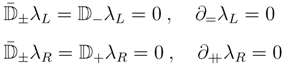
The N = (1,1) discussion of GHR identified the geometry of the sigma models that could be extended to have N = (2,2) supersymmetry, but they found closure of the algebra only when the complex structures commute, i.e., on ker[J(+), J(−)], in which case they gave a full N = (2,2) description in terms of chiral and twisted chiral fields. In this section we extend the discussion to the non-commuting case and describe the general situation following [32]. Earlier relevant discussions may be found in [61,62,63,64].
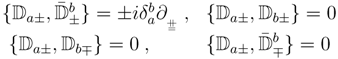
The d = 2, N = (2,2) algebra of covariant derivatives is
A chiral superfield ϕ satisfies the same constraints as in d = 4:
but in d = 2 we may also introduce twisted chiral fields χ that satisfy
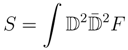
The sigma model action

then precisely yields the GKG on ker[J(+), J(−)], as may be seen by reducing the action to a N = (1,1)-formulation. Denoting the (1,1) covariant derivatives by D± and the generators of the second supersymmetry Q± we have
Note that this formulation shows that both the metric and the H-field have K as a potential

where derivatives on K are understood in the first line, and the second line is a three-form written in terms of the holomorphic differentials:

See [65] for a more detailed discussion of the above coordinatization.
Furthermore, as discussed for GKG in the previous section, the commuting complex structures imply the existence of a local product structure
To discriminate it from the general GK case we call this a “Bi-Hermitian Local Product” (BiLP) geometry.
The general case with (ker[J(+), J(−)])┴ ≠ ∅ was long a challenge. (In a number of publications co-authored by me, (ker[J(+), J(−)])┴ was incorrectly denoted coker[J(+), J(−)]. I apologize for participating in this misuse). The key issue here is what additional N = (2,2) superfields (if any) would suffice to describe the geometry. The available fields are complex linear ∑ϕ, twisted complex linear ∑χ and semichiral superfields. Of these ∑ϕ are dual to chirals and ∑χ to twisted chirals (See appendix A). The candidate superfields are thus left and right semi-(anti)chirals  which obey
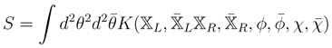
A N = (2,2) model written in terms of these fields reads
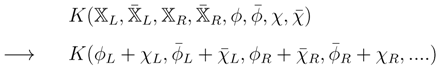
and an equal number of left and right fields are needed to yield a sensible sigma model. When reduced to N = (1,1) superspace, this action gives a more general model than what we have considered so far. Using Equation (94) we have the following N = (1,1) superfield content;
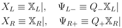
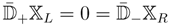
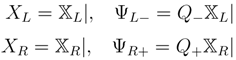
where the vertical bar now denotes setting half the fermi-coordinates to zero. Clearly, XL,R are scalar superfields and hence suitable for the N = (1,1) sigma model, but ΨL,R± are spinorial fields. They enter the reduced action as auxiliary fields and are the auxiliary N = (1,1) superfields needed for closure of the N = (2,2) algebra when [J(+), J(−)] ≠ 0 (see [12]). The structure of such an a N = (1,1) action is schematically [29]

where E = G + B as before.
In [32] we show that a sigma model fully describing GKG, i.e., ker[J(+), J(−)] ⊕ (ker[J(+), J(−)])┴, is (away from irregular points, i.e., points where the Poisson structures Equation (103), Equation (108) change rank)
where K acts as a generalized Kähler potential in terms of derivatives of which all geometric quantities can be expressed (locally). This Khas the additional interpretation as a generating function for symplectomorphisms between certain sets of coordinates on (ker[J(+), J(−)])┴, the canonical coordinates for J(+) and J(−), respectively. The proof of these statements relies heavily on Poisson geometry [32] and is summarized in what follows.
First, the fact that (ϕ,χ) and their Hermitian conjugates are enough to describe ker[J(+), J(−)] may be reformulated using the Poisson-structures [66]

In a neighborhood of a regular point, coordinates may be chosen such that

It can be shown that A ≠ A' and that we have coordinates labeled (a, a', A.A') adapted to

where

Here Ic and It have the canonical form

We thus have nice coordinates for ker[J(+) − J(−)] ⊕ ker[J(+) + J(−)] = ker[J(+), J(−)], but (ker[J(+), J(−)])┴ remains to be described. Here a third Poisson structure turns out to be useful;

Now kerσ = ker π+ ⊕ ker π− so we focus on (kerσ)┴. The symplectic leaf for σ is (ker[J(+), J(−)])┴ and the third Poisson structure also has the following useful properties [67]:

where the holomorphic types are with respect to both complex structures. To investigate the consequences of Equation (109) it is advantageous to first consider the case when ker[J(+), J(−)] = ∅. It then follows that σ is invertible and its inverse Ω is a symplectic form;

We may chose coordinates adapted to J(+)

In those coordinates we have from Equation (109) that

which identifies  as a holomorphic symplectic structure. The coordinates may then be further specified to be Darboux coordinates for this symplectic structure

The same derivation with J(+) replaced by J(−) gives a second set of Darboux coordinates which are canonical coordinates for J(−) and where

Clearly the two sets of canonical coordinates are related by a symplectomorphism. Let K(q, P) denote a generating function for this symplectomorphism. Expressing all our quantities in the mixed coordinates (q, P), we discover that the expressions for J(+), Ω, G = Ω[J(+), J(−)],… are precisely what we (see also [12,64] for partial results) derived from the sigma model action Equation (102) provided that we identify the coordinates (q, P) with (  ) (and the same for the Hermitian conjugates).
In the general case when [J(+), J(−)] ≠ ∅, we again get agreement, provided that the coordinates indexed Aand A' in Equation (106) are identified with the chiral and twisted chiral fields (ϕ, χ). We thus have a one to one correspondence between the description covered by the sigma model and all of [J(+), J(+)], i.e., for all possible cases.
10. Linearization of Generalized Kähler Geometry
The generalized Kähler potential  yields all geometric quantities, but as non-linear expressions (dualizing a BiLP to (twisted) complex linear fields yields a model with similar nonlinearities) in derivatives of K(unlike the case Equation (95)). In [34] we show that these non-linearities can be viewed as arising from a quotient of a higher dimensional model with certain null Kac–Moody symmetries. To illustrate the idea, we first consider an example.
10.1. A Bosonic Example
Consider a Lagrangian of the form

Following Stückelberg, we may think of this as a gauge fixed version of the gauge-invariant Lagrangian

with  and gauge invariance

Finally, the Lagrangian L2 can in turn be thought of as arising through gauging of the global translational symmetry δφ = ε in a third Lagrangian

A slightly more elaborate example is provided by the following sigma model Lagrangian;

where Aμ is an auxiliary field. Following the line of reasoning above, this Lagrangian may be thought of as a gauge fixed version of

where Dμ is as defined above, Ga0 ≡ Ga, G00 ≡ G and the Stückelberg field φ ≡ϕ0. In turn  is the gauged version (in adapted coordinates) of the Lagrangian

whose global symmetry is given by the isometry

We see that eliminating the auxiliary field in  is tantamount to extremizing with respect to the gauge field, i.e., to constructing a quotient of the Lagrangian
  with respect to its isometry. The only remaining question seems to be if varying the gauge-fixed is the same as varying (modulo gauge-fixing). The resulting Aμ’s differ by a gauge-transformation ∂μφ. Explicitly:

10.2. The Generalized Kähler Potential
We apply the procedure described above to a semichiral sigma model. Most of the rest of this section is taken directly from [34,35] where more details may be found.
Consider the generalized Kähler potential
where are left and right semi-chiral N = (2,2) superfields:
We descend to N = (1,1) as in Equation (100) by defining components
which satisfy


The N = (1,1) form of the Lagrangian is

where

Here we use a short hand notation where, e.g., KLR denotes the matrix of second derivatives of the potential Equation (124) with respect to both bared and un-bared left and right fields. Also the canonical complex structures Iis defined in Equation (107). Notice that neither ΨL+ nor ΨR− occur in the action.
10.3. ALP and Kac–Moody Quotient
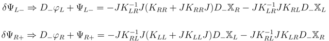
The procedure  outlined in Section 10.1 applied to the present case entails the replacements (ΨL−,ΨR+) ⟶ (∇−φL, ∇+φR) ⟶ (D−φL, D+φR) with given by Equation (129), and where

The gauge invariance of is

which gauges the following “global” invariance of :

Since the matrix E in Equation (130) is independent of φR/L, invariance under Equations (117) and (133) is immediate. Using the metric  one also verifies that the Killing-vectors

are null-vectors. Furthermore, the constraints in Equation (133) imply

or covariantly [68]

with ∇(±) defined in Equation (73). These relations identify the global symmetries as null Kac–Moody isometries.
After applying the procedure outlined above, we obtain a Lagrangian . It is then useful to introduce a definition from [34]:
The space corresponding to is the N = (1,1)form of the Auxiliary Local Product space (ALP) for the N = (2,2)Lagrangian in Equation (129).
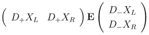
In other words, the ALP is given by the action

where E is the matrix given in Equation (130), the bullets denote the decoupled ΨL+,ΨR−, and the Lagrangian is invariant under the global Kac–Moody isometry Equation (134).
10.3.1. Kac–Moody Quotient in (1,1)
The Lagrangian Equation (137) is an equivalent starting point for deriving the GK geometry for the target space of Equation (129): To recapitulate from Section 10.1, this proceeds by gauging the isometry to obtain the Lagrangian

Elimination of the gauge fields (cf. Equation (123));
yields the quotient metric and B-field from E:

where, suppressing indices on the two by two complex matrices,

The corresponding Lagrangian is
10.3.2. Kac–Moody quotient in (2,2)
As an alternative, we may perform the Kac–Moody quotient in (2,2) superspace. Very briefly, this goes as follows:
In the generalized potential we replace the semi-chiral fields by sums of chiral and twisted chiral fields according to
This doubles the degrees of freedom in the semi sector but the corresponding action has a Kac–Moody symmetry

where the parameters satisfy
To keep the same degrees of freedom as in the original model, we gauge the Kac–Moody symmetry which reintroduces semi-chiral fields:

The local complex Kac–Moody symmetry is now

The equivalence to the generalized potential is seen by going to a gauge where the “ϕ + χ” terms are zero.
For comparison, we descend to N = (1,1) via the identification

This gives the N = (1,1) action in terms of the complex scalar fields XL,R and φL,R, with the Kac–Moody generated by the null Killing vectors Equation (134). These corresponding isometries may be used in a quotient to give precisely the nonlinear expressions in terms of derivatives of K that we found in Equation (140). They arise from

where Eμv are the XL,R components in Equation (130). Note that the existence of a left and a right isometry generalizes the construction in Equation (44) slightly, to allow for a B-field.
11. Projective Superspace
Typically, the N = (2,2) formulation of the N = (4,4) models require explicit transformations on the N = (2,2) superfields that close to the supersymmetry algebra on-shell. This non-manifest formulation makes the construction of new models difficult. Below follows a brief description of a superspace where all supersymmetries are manifest. This projective superspace (The name refers to the projective coordinates on ℂℙ1 =∶ ℙ1 being used. It is really a misnomer in that it is unrelated to the usual definition of projective spaces) [6,7,8,9,10,11,12,13,14,15,16,17,18,19] has been developed independent of harmonic superspace [69]. The relation between the two approaches was first discussed in [70] and more recently in [71]. A key reference for this section is [72] and the review [73].
A hyperkähler space Tsupports three globally defined integrable complex structures I, J, K obeying the quaternion algebra: IJ =−JI =K, plus cyclic permutations. Any linear combination of these aI +bJ +cK is again a complex structure on Tif a2 + b2 + c2 = 1, i.e., if {a,b,c} lies on a two-sphere S2 ≃ ℙ1. The Twistor space Zof a hyperkähler space Tis the product of Twith this two-sphere Z = T × ℙ1. The two-sphere thus parametrizes the complex structures and we choose projective coordinates  to describe it (in a patch including the north pole). It is an interesting and remarkable fact that the very same S2 arises in an extension of superspace to accommodate manifest N = (4,4) models.
Although projective superspace can be defined for different bosonic dimensions, we shall remain in two. Here the algebra of N = (4,4) superspace derivatives is
We may parameterize a ℙ1 of maximal graded Abelian sub-algebras as (suppressing the spinor indices)

where is the coordinate introduced above, and the bar on ∇ denotes conjugation with respect to a real structure ℜ defined as complex conjugation composed with the antipodal map on ℙ1 ≃ S2. The two new covariant derivatives in Equation (151) anti-commute

They may be used to introduce constraints on superfields similarly to how the N = (2,2) derivatives are used to impose chirality constraints in Section 9. Superfields now live in an extended superspace with coordinates  . The superfields ϒ we shall be interested in satisfy the projective chirality constraint

and are taken to have the following -expansion:

When the index i ∈ [0, ∞) the field ϒ is analytic around the north pole of the ℙ1 and consequently called an arctic multiplet. For tropical and antarctic multiplets see [17]. We use the real structure acting on superfields,  , to impose reality conditions on the superfields. An O(2n) multiplet is thus defined via

The expansion Equation (154) is useful in displaying the N = (2,2) content of the multiplets. Using the relation Equation (151) to the N = (2,2) derivatives in Equation (153) we read off the following expansion for an O(4) multiplet Equation (155):

with the component N = (2,2) fields being chiral ϕ, unconstrained Xand complex linear Σ. A complex linear field satisfies

and is dual to a chiral superfield (see the appendix). A general arctic projective chiral ϒ has the expansion

with all Xi’s unconstrained.
11.1. The Generalized Legendre Transform
In this section we review one particular construction of hyperkähler metrics using projective superspace introduced in [11].
An N = (4,4) invariant action for the field in Equation (158) may be written as
with

for some suitably defined contour C. Eliminating the auxiliary fields Xi by their equations of motion will yield an N = (2,2) model defined on the tangent bundle T(T) parametrized by (ϕ, Σ). Dualizing the complex linear fields Σ to chiral fields the final result is a supersymmetric N = (2,2) sigma model in terms of  which is guaranteed by construction to have N = (4,4) supersymmetry, and thus to define a hyperkähler metric. In equations, these steps are:
Solve the equations of motion for the auxiliary fields (techniques for this were developed in [74]):

Solving these equations puts us on N = 2-shell, which means that only the N = (2,2) component symmetry remains off-shell. (In fact, insisting on keeping the N = (4,4) constraints Equation (153) will put us totally on-shell.) In N = (2,2) superspace the resulting model, after eliminating Xi, is given by a Lagrangian  . This is finally dualized to
  via a Legendre transform

11.2. Hyperkähler Metrics on Hermitian Symmetric Spaces
This section contains an introduction to [26] where the generalized Legendre transform described in the previous section is used to find metrics on the Hermitian symmetric spaces listed in the following table:
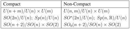
The special features of these quotient spaces that allow us to find a hyperkähler metric on their co-tangent bundle is the existence of holomorphic isometries and that we are able to find convenient coset representatives.
A simple example of how the coset representative enters in understanding a quotient is given, e.g., in [75]. In  the sphere Sn forms a representation of SO(n + 1). The isotropy subgroup at the north pole p0 of Sn is SO(n). Consider another point p on Sn and let gp ∈SO(n + 1) be an element that maps p0 ⟶ p. The complete set of elements of SO(n + 1) which map p0 ⟶ p is thus of the form gpSO(n), or in other words Sn = SO(n + 1)/SO(n). A coset representative is a choice of element in gpSO(n), and that choice can make the transport of properties defined at the north pole to an arbitrary point more or less transparent.
An important step in the generalized Legendre transform is to solve the auxiliary field Equation (161). As outlined in [74] and further elaborated in [76], for Hermitian symmetric spaces the auxiliary fields may be eliminated exactly. In the present case, we start from a solution at the origin ϕ = 0,

We then extend this solution to a solution ϒ* at an arbitrary point using a coset representative. We illustrate the method in an example due to S. Kuzenko.
Ex. (Kuzenko)
The Kähler potential for ℙ1 is given by

and we denote the metric that follows from this by  . Here ϕ is a holomorphic coordinate which we extend to an N = (2,2) chiral superfield. To construct a hyperkähler metric we first replace ϕ ⟶ ϒ, and then solve the auxiliary field equation as in Equation (163). Thinking of ℂℙn as the quotient G1,n+1(ℂ) = U(n + 1)/U(n) × U(1), we use a carefully chosen coset representative
  to extend the solution from the origin to an arbitrary point. The result is

To find the chiral multiplet Σ that parametrizes the tangent bundle, we use the definition

yielding

The N = (2,2) superspace Lagrangian on the tangent bundle is then

The final Legendre transform replacing the linear multiplet by a new chiral field  produces the Kähler potential
  for the Eguchi–Hanson metric.
The ℙ1 example captures the essential idea in our construction. The reader is referred to the papers [26,27,28] for more examples.
11.3. Other Alternatives in Projective Superspace
Of the two methods for constructing hyperkähler metrics introduced in [4], we have dwelt on the Legendre transform generalized to projective superspace. The hyperkähler reduction discussed in Section 6 may also be lifted to projective superspace. Both these methods involve only chiral N = (2,2) superfields. When a nonzero B-field is present, the N = (2,2) sigma models involve chiral, twisted chiral and semichiral superfields, as discussed in Section 2. For a full description of (generalizations of) hyperkähler metrics on such spaces, the doubly projective superspace [12] is required. We now briefly touch on this construction.
In the doubly projective superspace, at each point in ordinary superspace we introduce one ℙ1 for each chirality and denote the corresponding coordinates by  and
and  . The condition Equation (151) turns into
with the conjugated operators defined with respect to the real structure ℜ acting on both and . A superfield has the expansion

and is taken to be both left and right projectively chiral. We may also impose reality conditions using ℜ, as well as particular conditions on the components, such as the “cylindrical” condition

for some k. Actions are formed in analogy to Equations (159) and (160). The N = (2,2) components of such a model include twisted chiral fields χ, as well as semi-chiral ones . In fact this is the context in which the semi-chiral N = (2,2) superfields were introduced [12]. Hyperkähler metrics derived in this superspace are discussed in [14]. An exciting project is to merge this picture with the results in [34].
Appendix
A. Chiral-Complex linear duality
In two dimensions, chiral superfields Equation (13) obey

and twisted chiral superfields χ obey
and the complex conjugate relations. They are related via Legendre transformations to complex linearΣϕ and twisted complex linear Σχ superfields obeying
and the complex conjugate relations.
A parent action which relates a BiLP generalized Kähler potential  to its dual
  is
is

Variation of the (twisted) complex linear fields constrains  to be
to be  and is recovered. On the other hand, the field equations are

Assuming that they can be solved for as functions of the (twisted) complex linear fields we find the Legendre transformed potential when the solutions are plugged back into Equation (A4).
The above discussion is purely local. To consider global issues, one must take into account gluing of the potential between patches. In the BiLP case the allowed change between patches Oa and Ob is given by holomorphic coordinate transformations the (generalized) Kähler gauge transformations.
Let us look at Kähler gauge transformations, restricting to the case with no twisted chiral fields for simplicity. We thus have

which via a holomorphic coordinate transformation ϕ' = F(ϕ) is equivalent to

One may ask what this freedom corresponds to in the dual model where no ambiguity of the same type exists.
The dual to K is found from the Legendre transform with parent action

and reads

after solving

The parent action to is best considered after the coordinate transformation Equation (7):

where  . We find the corresponding dual potential

after solving

Comparing to Equation (A10) we see that  as a functions of X is related to Σϕ as a function of X via a holomorphic coordinate transformation depending on the Kähler gauge transformation Fand similarly for their complex conjugate. Explicitly

The relation between  and
and  is more complicated due to the linear X terms, but can be worked out from Equations (A12) and (A9).
Acknowledgment
I am very happy to acknowledge all my collaborators on the papers that form the basis of this presentation. In particular I am grateful for the many years of continuous collaboration with Martin Roček, my intermittent collaborations with Chris Hull, as well as the also long but more recent collaborations with Sergei Kuzenko, Rikard von Unge and Maxim Zabzine. The figure from [5] is reproduced with permission from Springer Verlag. The work was supported by VR grant 621-2009-4066.
References
- Gell-Mann, M.; Levy, M. The axial vector current in beta decay. Nuovo Cimento 1960, 16, 705–726. [Google Scholar] [CrossRef]
- Zumino, B. Supersymmetry and kahler manifolds. Phys. Lett. B 1979, 87, 203–206. [Google Scholar] [CrossRef]
- Alvarez-Gaumé, L.; Freedman, D.Z. Geometrical structure and ultraviolet finiteness in the supersymmetric sigma model. Commun. Math. Phys. 1981, 80, 443–451. [Google Scholar] [CrossRef]
- Lindström, U.; Roček, M. Scalar tensor duality and N = 1, 2 nonlinear sigma-models. Nucl. Phys. B 1983, 222, 285–308. [Google Scholar] [CrossRef]
- Hitchin, N.J.; Karlhede, A.; Lindström, U.; Roček, M. Hyperkahler metrics and supersymmetry. Commun. Math. Phys. 1987, 108, 535–589. [Google Scholar] [CrossRef]
- Karlhede, A.; Lindström, U.; Roček, M. Selfinteracting tensor multiplets in N = 2 superspace. Phys. Lett. B 1984, 147, 297–300. [Google Scholar]
- Gates, S.J.; Hull, C.M.; Roček, M. Twisted multiplets and new supersymmetric nonlinear sigma models. Nucl. Phys. B 1984, 248, 157–186. [Google Scholar] [CrossRef]
- Grundberg, J.; Lindström, U. Actions for linear multiplets in six-dimensions. Class. Quantum Gravity 1985, 2, L33. [Google Scholar] [CrossRef]
- Karlhede, A.; Lindström, U.; Roček, M. Hyperkahler manifolds and nonlinear supermultiplets. Commun. Math. Phys. 1987, 108, 529–534. [Google Scholar] [CrossRef]
- Lindström, U. Generalized N = (2,2) supersymmetric nonlinear sigma models. Phys. Lett. 2004, B587, 216–224. [Google Scholar]
- Lindström, U.; Roček, M. New hyperkahler metrics and new supermultiplets. Commun. Math. Phys. 1988, 115, 21–29. [Google Scholar] [CrossRef]
- Buscher, T.; Lindström, U.; Roček, M. New supersymmetric sigma models with wess-zumino terms. Phys. Lett. B 1988, 202, 94–98. [Google Scholar] [CrossRef]
- Lindström, U.; Roček, M. N = 2 super yang-mills theory in projective superspace. Commun. Math. Phys. 1990, 128, 191–196. [Google Scholar] [CrossRef]
- Lindström, U.; Ivanov, I.T.; Roček, M. New N = 4 superfields and sigma models. Phys. Lett. B 1994, 328, 49–54. [Google Scholar] [CrossRef]
- Lindström, U.; Kim, B.; Roček, M. The Nonlinear multiplet revisited. Phys. Lett. B 1995, 342, 99–104. [Google Scholar] [CrossRef]
- Ivanov, I.T.; Roček, M. Supersymmetric sigma models, twistors, and the Atiyah-Hitchin metric. Commun. Math. Phys. 1996, 182, 291–302. [Google Scholar] [CrossRef]
- Gonzalez-Rey, F.; Roček, M.; Wiles, S.; Lindström, U.; von Unge, R. Feynman rules in N = 2 projective superspace. (I). Massless hypermultiplets. Nucl. Phys. B 1998, 516, 426–448. [Google Scholar] [CrossRef]
- Gonzalez-Rey, F.; von Unge, R. Feynman rules in N = 2 projective superspace. (II). Massive hypermultiplets. Nucl. Phys. B 1998, 516, 449–466. [Google Scholar] [CrossRef]
- Gonzalez-Rey, F. Feynman rules in N = 2 projective superspace. III: Yang-Mills multiplet. 1997, arXiv:hep-th/9712128. Available online: http://arxiv.org/abs/hep-th/9712128 (accessed on 14 August 2012).
- Kuzenko, S.M.; Tartaglino-Mazzucchelli, G. 5D supergravity and projective superspace. J. High Energy Phys. 2008. [Google Scholar] [CrossRef]
- Kuzenko, S.M.; Lindström, U.; Roček, M.; Tartaglino-Mazzucchelli, G. 4D N = 2 supergravity and projective superspace. J. High Energy Phys. 2008. [Google Scholar] [CrossRef]
- Kuzenko, S.M. On N = 2 supergravity and projective superspace: Dual formulations. Nucl. Phys. B 2009, 810, 135–149. [Google Scholar] [CrossRef]
- Kuzenko, S.M.; Lindström, U.; Roček, M.; Tartaglino-Mazzucchelli, G. On conformal supergravity and projective superspace. J. High Energy Phys. 2008. [Google Scholar] [CrossRef]
- Tartaglino-Mazzucchelli, G. 2D N = (4,4) superspace supergravity and bi-projective superfields. J. High Energy Phys. 2010. [Google Scholar] [CrossRef]
- Linch, W.D.; Tartaglino-Mazzucchelli, G., III. Six-dimensional supergravity and projective superfields. 2012, arXiv:1204.4195. Available online: http://arxiv.org/abs/1204.4195 (accessed on 14 August 2012).
- Arai, M.; Kuzenko, S.M.; Lindström, U. Hyperkaehler sigma models on cotangent bundles of Hermitian symmetric spaces using projective superspace. J. High Energy Phys. 2007. [Google Scholar] [CrossRef]
- Arai, M.; Kuzenko, S.M.; Lindström, U. Polar supermultiplets, Hermitian symmetric spaces and hyperkahler metrics. J. High Energy Phys. 2007. [Google Scholar] [CrossRef]
- Kuzenko, S.M.; Novak, J. Chiral formulation for hyperkahler sigma-models on cotangent bundles of symmetric spaces. J. High Energy Phys. 2008. [Google Scholar] [CrossRef]
- Lindström, U. Generalized N = (2,2) supersymmetric nonlinear sigma models. Phys. Lett. B 2004, 587, 216–224. [Google Scholar] [CrossRef]
- Lindström, U.; Minasian, R.; Tomasiello, A.; Zabzine, M. Generalized complex manifolds and supersymmetry. Commun. Math. Phys. 2005, 257, 235–256. [Google Scholar] [CrossRef]
- Lindström, U.; Roček, M.; von Unge, R.; Zabzine, M. Generalized Kahler geometry and manifest N = (2,2) supersymmetric nonlinear sigma-models. J. High Energy Phys. 2005. [Google Scholar] [CrossRef]
- Lindström, U.; Roček, M.; von Unge, R.; Zabzine, M. Generalized Kahler manifolds and off-shell supersymmetry. Commun. Math. Phys. 2007, 269, 833–849. [Google Scholar]
- Bredthauer, A.; Lindström, U.; Persson, J.; Zabzine, M. Generalized Kahler geometry from supersymmetric sigma models. Lett. Math. Phys. 2006, 77, 291–308. [Google Scholar] [CrossRef]
- Lindström, U.; Roček, M.; von Unge, R.; Zabzine, M. Linearizing generalized Kahler geometry. J. High Energy Phys. 2007. [Google Scholar] [CrossRef]
- Lindström, U.; Roček, M.; von Unge, R.; Zabzine, M. A potential for Generalized Kahler Geometry. IRMA Lect. Math. Theor. Phys. 2010. [Google Scholar] [CrossRef]
- Lindström, U.; Roček, M.; Ryb, I.; von Unge, R.; Zabzine, M. T-duality and Generalized Kahler Geometry. J. High Energy Phys. 2008. [Google Scholar] [CrossRef]
- Hull, C.M.; Lindström, U.; Roček, M.; von Unge, R.; Zabzine, M. Generalized Kahler geometry and gerbes. J. High Energy Phys. 2009. [Google Scholar] [CrossRef]
- Göteman, M.; Lindström, U. Pseudo-hyperkahler Geometry and Generalized Kahler Geometry. Lett. Math. Phys. 2011, 95, 211–222. [Google Scholar] [CrossRef]
- Göteman, M.; Lindström, U.; Roček, M.; Ryb, I. Sigma models with off-shell N=(4,4) supersymmetry and noncommuting complex structures. J. High Energy Phys. 2010. [Google Scholar] [CrossRef]
- Hull, C.M.; Lindström, U.; Roček, M.; von Unge, R.; Zabzine, M. Generalized Calabi-Yau metric and Generalized Monge-Ampere equation. J. High Energy Phys. 2010. [Google Scholar] [CrossRef]
- Hull, C.M.; Lindström, U.; Roček, M.; von Unge, R.; Zabzine, M. Generalized Kähler Geometry in (2,1) superspace. J. High Energy Phys. 2012. [Google Scholar] [CrossRef]
- Craps, B.; Roose, F.; Troost, W.; van Proeyen, A. What is special Kahler geometry? Nucl. Phys. B 1997, 503, 565–613. [Google Scholar] [CrossRef]
- Albertsson, C.; Lindström, U.; Zabzine, M. N = 1 supersymmetric sigma model with boundaries, I. Commun. Math. Phys. 2003, 233, 403–421. [Google Scholar]
- Albertsson, C.; Lindström, U.; Zabzine, M. N = 1 supersymmetric sigma model with boundaries. II. Nucl. Phys. B 2004, 678, 295–316. [Google Scholar] [CrossRef]
- Lindström, U.; Roček, M.; van Nieuwenhuizen, P. Consistent boundary conditions for open strings. Nucl. Phys. B 2003, 662, 147–169. [Google Scholar] [CrossRef]
- Howe, P.S.; Lindström, U.; Wulff, L. Superstrings with boundary fermions. J. High Energy Phys. 2005. [Google Scholar] [CrossRef]
- Hull, C.M. Lectures on Nonlinear Sigma Models and Strings. In Proceedings of the Lectures Give at Vancouver Theory Workshop, Vancouver, Canada, 25 July-6 August, 1986; p. 77.
- Gates, S.J.; Grisaru, M.T.; Roček, M.; Siegel, W. Superspace or one thousand and one lessons in supersymmetry. Front. Phys. 1983, 58, 1–548. [Google Scholar]
- Wess, J.; Bagger, J. Supersymmetry and Supergravity; World Scientific: Princeton, NJ, USA, 1992; p. 259. [Google Scholar]
- Buchbinder, I.L.; Kuzenko, S.M. Ideas and Methods of Supersymmetry and Supergravity: Or a Walk Through Superspace; Taylor & Francis: Bristol, UK, 1998; p. 656. [Google Scholar]
- Salam, A.; Strathdee, J.A. Supergauge transformations. Nucl. Phys. B 1974, 76, 477–482. [Google Scholar] [CrossRef]
- Berezin, F.; Leites, D. Supermanifolds. Soviet Maths Doklady 1976, 16, 1218–1222. [Google Scholar]
- Berezin, F.A. The Method of Second Quantization; Academic Press: Waltham, MA, USA, 1966. [Google Scholar]
- Hull, C.M.; Karlhede, A.; Lindström, U.; Roček, M. Nonlinear sigma models and their gauging in and out of superspace. Nucl. Phys. B 1986, 266, 1–44. [Google Scholar] [CrossRef]
- Hull, C.M.; Witten, E. Supersymmetric sigma models and the heterotic string. Phys. Lett. 1985, B160, 398–402. [Google Scholar]
- Guillemin, V.; Sternberg, S. Symplectic Techniques in Physics; Cambridge University Press: Cambridge, UK, 1984. [Google Scholar]
- Hull, C.M.; Papadopoulos, G.; Spence, B.J. Gauge symmetries for (p,q) supersymmetric sigma models. Nucl. Phys. B 1991, 363, 593–621. [Google Scholar] [CrossRef]
- Hull, C.M.; Papadopoulos, G.; Townsend, P.K. Potentials for (p,0) and (1,1) supersymmetric sigma models with torsion. Phys. Lett. B 1993, 316, 291–297. [Google Scholar] [CrossRef]
- Hitchin, N. Generalized Calabi-Yau manifolds. Q. J. Math. 2003, 54, 281–308. [Google Scholar] [CrossRef]
- Gualtieri, M. Generalized Complex Geometry. Ph.D. Thesis, Oxford University, Oxford, UK, 2004. [Google Scholar]
- Sevrin, A.; Troost, J. The geometry of supersymmetric sigma models. In Proceedings of the Workshop Gauge Theories, Applied Supersymmetry and Quantum Gravity, Imperial College, London, 5-10 July, 1996.
- Sevrin, A.; Troost, J. Off-shell formulation of N = 2 nonlinear sigma models. Nucl. Phys. B 1997, 492, 623–646. [Google Scholar] [CrossRef]
- Grisaru, M.T.; Massar, M.; Sevrin, A.; Troost, J. The Quantum geometry of N = (2,2) nonlinear sigma models. Phys. Lett. B 1997, 412, 53–58. [Google Scholar] [CrossRef]
- Bogaerts, J.; Sevrin, A.; van der Loo, S.; van Gils, S. Properties of semichiral superfields. Nucl. Phys. B 1999, 562, 277–290. [Google Scholar] [CrossRef]
- Ivanov, I.T.; Kim, B.; Roček, M. Complex structures, duality and WZW models in extended superspace. Phys. Lett. 1995, B343, 133–143. [Google Scholar]
- Lyakhovich, S.; Zabzine, M. Poisson geometry of sigma models with extended supersymmetry. Phys. Lett. 2002, B548, 243–251. [Google Scholar]
- Hitchin, N. Instantons, Poisson structures and generalized Kähler geometry. Commun. Math. Phys. 2006, 265, 131–164. [Google Scholar] [CrossRef]
- Roček, M.; Verlinde, E.P. Duality, quotients, and currents. Nucl. Phys. B 1992, 373, 630–646. [Google Scholar] [CrossRef]
- Galperin, A.S.; Ivanov, E.A.; Ogievetsky, V.I.; Sokatchev, E.S. Harmonic Superspace; Cambridge University Press: Cambridge, UK, 2001; p. 306. [Google Scholar]
- Kuzenko, S.M. Projective superspace as a double-punctured harmonic superspace. Int. J. Mod. Phys. A 1999, 14, 1737–1758. [Google Scholar] [CrossRef]
- Jain, D.; Siegel, W. Deriving projective hyperspace from harmonic. Phys. Rev. D 2009, 80, 045024:1–045024:9. [Google Scholar]
- Lindström, U.; Roček, M. Properties of hyperkahler manifolds and their twistor spaces. Commun. Math. Phys. 2010, 293, 257–278. [Google Scholar] [CrossRef]
- Kuzenko, S.M. Lectures on nonlinear sigma-models in projective superspace. J. Phys. A Math. Theor. 2010, 43, 443001. [Google Scholar] [CrossRef]
- Gates, S.J., Jr.; Kuzenko, S.M. The CNM-hypermultiplet nexus. Nucl. Phys. B 1999, 543, 122–140. [Google Scholar] [CrossRef]
- Van Nieuwenhuizen, P. General Theory of Coset Manifolds and Antisymmetric Tensors Applied to Kaluza-Klein Supergravity; Trieste School: Trieste, Italy, 1984. [Google Scholar]
- Kuzenko, S.M. Extended supersymmetric nonlinear sigma-models on cotangent bundles of Kähler manifolds: Off-shell realizations, gauging, superpotentials. In Talks given at the University of Munich, Imperial College, Cambridge University, May-June 2006.
© 2012 by the authors; licensee MDPI, Basel, Switzerland. This article is an open-access article distributed under the terms and conditions of the Creative Commons Attribution license (http://creativecommons.org/licenses/by/3.0/).
Share and Cite
Lindström, U. Supersymmetric Sigma Model Geometry. Symmetry 2012, 4, 474-506. https://doi.org/10.3390/sym4030474
Lindström U. Supersymmetric Sigma Model Geometry. Symmetry. 2012; 4(3):474-506. https://doi.org/10.3390/sym4030474
Chicago/Turabian StyleLindström, Ulf. 2012. "Supersymmetric Sigma Model Geometry" Symmetry 4, no. 3: 474-506. https://doi.org/10.3390/sym4030474
APA StyleLindström, U. (2012). Supersymmetric Sigma Model Geometry. Symmetry, 4(3), 474-506. https://doi.org/10.3390/sym4030474