1. Introduction
There are eleven sections in this paper. The first six sections—not quite half of the paper—develop the subject model.
Section 7 relates and contrasts that model with the Standard Model in terms of the particles and interactions most commonly encountered and
Section 8 extends the discussion to the triplication of particles and interactions observed in the high energy domain.
Section 10 is a recapitulation and summation and
Section 11 summarizes some connections to additional topics of interest. Six subjects have been relegated to the back as appendices mainly because they are a bit more mathematically detailed (rather than of intrinsically lesser import.
Two items need mention before we begin to validate the abstract. First an acknowledgement: due to the nature of this paper, it is necessary to describe in considerable detail the subject model whose development has been similarly described in references [
1,
2,
3,
4]. The large amount of overlap thus precludes a
detailed citation of those references except as explicitly indicated. Additional sources are cited as the referenced material occurs in the text.
Next, a question, one that increasingly emerges in various guises at the frontiers of physics: “Just exactly what
is an elementary particle?” Even though it evokes such matters as the meaning of the word “is”, this is not a frivolous question
1; indeed for the model to be described herein it’s fundamental. The celebrated nobelist Eugene Wigner who did so much to advance the role of symmetry in physics is credited with a detailed
algebraic analysis of the subject with the conclusion that an “elementary particle “is” an irreducible unitary representation of the group, G. of physics, that is, the double (universal) cover of the Poincare group of those transformations of special relativity which can be continuously deformed to the identity” [
5]. However, this is really an epistemological definition, useful for enumerating the attributes necessary for identifying a particle as elementary but providing scant guidance for describing, say, the nature of the particulate occupation of space, in some ontologically satisfying way.
Actually, the notion that there even are such things as elementary particles goes back (but apparently no further) to the fifth century BCE and the Greek philosopher Democritus for whom all matter was “composed of many different kinds of minute hard particles.” [
6]. His particles were supposed to be so small that they couldn’t be seen and so hard that they were “atomos”, that is, not susceptible to further subdivision. Nor, was it possible in antiquity to endow such “atoms” with additional attributes, certainly not with form or internal structure.
The notion of the atomicity of matter then languished for centuries. We are told that Isaac Newton in the seventeenth century also believed all matter to be somehow composed of infinitely small, infinitely hard atoms. Eventually, chemists found it expedient to postulate various kinds of elementary particles—atoms—each with a particular mass and electric charge in order to explain the variety of the substances of their experience. By the middle of the nineteenth century, a great variety of atoms were recognized and there was even an attempt to associate form and structure to them to explain the variety (see below). Nevertheless, it was not until the early twentieth century that most of the skepticism regarding the existence of atoms was dispelled. Albert Einstein’s explanation of Brownian motion was a big help in that regard. Nowadays, we have the technology that lets us “see” atoms, we know the mechanics of how they combine in the various forms of matter and we have a detailed taxonomy of atoms organized in terms of their internal structure; atoms are no longer elementary.
In fact, neither are all their immediate constituents. In the paradigmatic Standard Model (SM) of particle physics electrons are still elementary but the nucleons, that is the neutrons and protons, are endowed with an elaborate internal structure for which the ultimate elementarity resides in infinitesimal point particles, the quarks. For the time being anyway, the process of “reduction”—attributing behavior at one level to a further level of composition—seems to have ceased, or at least greatly diminished and it is the electrons (more generally the leptons) and the quarks that are considered to be “atomos”, structureless and without form.
Thus, although its elementary particles satisfy the Wigner criterion for elementarity, the SM simply takes the ontological default position for which those particles are still just featureless, infinitesimal points, a position fraught with mathematical complexity. While it is undeniable that no form or structure can yet be discerned for the electron, and that quarks evidently cannot be detected outside their nucleonic housing (ergo, additional theory to explain
why they are so confined), the net result in addition to complexity, is the need to assign values to a host of parameters and even to
postulate the existence of an ineffable, enigmatic additional particle so as to impart the vital attribute of mass to known particles.
2Which brings us to our model, the subject of this paper. As we shall see, this is a model for which particle attributes and particle conformation in space are
linked, inherently and inseperably. At this point, we can do no better in summing up the model’s approach than to quote the following from the introduction to a paper published in a knot theory journal [
1]: “The connection between knot theory and physics is well documented.—Here, beginning with two rudimentary knots, the unknot and the trefoil knot, we develop a unique approach to understanding the elementary particles of physics in terms of a visualizable reduction of all particles—fermions and bosons, hadrons and leptons—to a common topology.—particles are regarded not as discrete, pointlike objects in a vacuum but as
localized distortions in and of an otherwise featureless continuum that supports torsion as well as curvature”.
But before we delve any further into the particulars of the model, we should mention one more bit of history, an early connection between knot theory and physics. This is the attempt in the mid nineteenth century by William Thompson, Lord Kelvin (in a sense, anticipating our model by something like a century and a half) to associate structure to the atoms known to exist at that time [
7]. In essence, Kelvin’s notion was that each atom
is a knot, one of the knots known at that time, somehow sustainable in the substance of the ether, the name given to the medium for the propagation of James Clerk Maxwell’s electromagnetic waves. Given Kelvin’s influence, the idea attracted considerable interest and some prominent adherents (including Maxwell himself). It also led to a determined effort to tabulate the variety of all possible knots but the demise of Kelvin’s vision was inevitable; he could not have known that atoms are composite.
However, since we do, the model to be described therefore associates form and structure explicitly to those atomic constituents, the leptons and nucleons and their combinations and interactions. And it is there that the process of reduction stops; we must emphasize that there are no quarks in this model. Consequently, there are no gluons to prevent a quark from wandering outside the confines of a nucleon. Nor is there a color SU(3) gauge theory to explain why the Pauli exclusion principle is not violated by a grouping of identical quarks. Nor, as we shall see, is there any need in the model for any of the above: neither quarks nor gluons nor color. And, finally, there is no need to import an additional particle in order to account for the mass of the particles that are modeled. As will be discussed in what follows, their mass emerges simply as part of their nature; they exist and persist as solitonic distortions of spacetime itself, in consonance with the dictates of general relativity.
Going back to the quotation noted above, the knots in question are
torus knots, specifically (2,
n) torus knots, and in fact the simplest members of that genre. In a sense, it may not be too far off the mark to credit the model’s existence to an underlying toroidal topology.
Figure 1 is a generic representation of a knot encircling a torus. The position of a point sliding along the knot is the vector
![Symmetry 04 00039 i001]()
. To close the knot, vector
![Symmetry 04 00039 i002]()
makes
n (meridianal) revolutions about the centerline of the toroidal core as vector
![Symmetry 04 00039 i003]()
revolves twice (longitudinally) around the central axis of that centerline. That is,
θ covers 2
πn radians while
ϕ covers 4
π radians. In Cartesian coordinates this is
where w = R + rcosθ and θ = n ϕ/2.
Figure 1.
A knot encircling a torus.
Figure 1.
A knot encircling a torus.
A clarification is appropriate here: the actual form and structure of the particles of the model are those of the
Moebius strip (MS) rather than of knots
per se. (In fact the MS will also be flattened and referred to as an FMS but we need to defer that for the moment). Nevertheless, the quotation above is accurate; there is an isomorphism between MS and (2,
n) torus knots such that the number of half twists, NHT, of the strip is
identical to the number,
n, of meridianal revolutions,
θ, of the knot that forms the strips
boundary. Thus, the boundary of the canonical MS with a single half twist (NHT = 1) is the folded-over unknot which, as shown in
Figure 2, requires two revolutions in space for a point sliding along the knot to complete one complete traversal of the knot itself. Correspondingly, an oriented figure on the surface of the MS must make two traversals of the strip in order to return to its original location and orientation.
Which evokes another point of emphasis: it is this two-to-one feature that qualifies either the MS or its knot border as the prototypical manifestation of the double coverage of the group SO(3) of rotations in 3-space by the gauge group SU(2), a group associated with spin in multiples of 1/2 and, as we shall see, the group that governs the top- level taxonomical development of the particles of the model. In effect, our model thus promotes the MS genus (or the corresponding knot genus) from its exemplary role to that of the basis for model development.
Figure 2.
A Moebius strip (MS) and its boundary.
Figure 2.
A Moebius strip (MS) and its boundary.
We should point out that it is not only the MS border that is knotlike; we can also view an MS as a
concatenation of (2,
n) torus knots and we can illustrate that notion by letting the toroidal core radius,
r, vary from zero up to some maximum value as we implement Equations 1-1.
Figure 3 shows the result for the trefoil (NHT = 3) using a discrete number of radii (In this case three).
Figure 3.
An MS as a concatenation of torus knots.
Figure 3.
An MS as a concatenation of torus knots.
Thus, concatenation is one way to “
frame” a knot in order to create an MS. Another approach to framing is to exploit
Alexander’s theorem [
8], which says that every knot or link can be represented as a braid with
closure. In our case we are concerned with the simplest braids involving only two strands as shown in
Figure 4 and closure means that the top and bottom ends of each braid in the column on the left are looped around and brought together as indexed left to right with the result shown in the next two columns (the right hand column being the usual portrayal).
The figure illustrates a number of relationships: the result for n = −1 is the folded over unknot (no twist) with one crossover while n = −3 gives the trefoil with three crossovers (The minus sign means a twist to the left), for n = 0 we get a pair of unlinked loops while for n = −2, the two loops are linked together at two crossovers. These results are examples of two general rules: odd and even values of n yield knots and links, respectively, and the number of crossings correlates with knot/link parameter n.
Figure 4.
Braids with closure and framing.
Figure 4.
Braids with closure and framing.
Also apparent is the requirement for two traversals to return to the origin in the case of all odd n but only one traversal for all even n, a requirement readily deducible from Equation 1-1. (e.g., The reference condition is w = R + r cosθ = R + r when θ = 0. Now, if we let θ = n ϕ/2 and ϕ = 2π, then w = R ± r when n is even or odd, respectively.) Also, notice the dotted lines in the figure, reminiscent of “rungs” on a ladder; if we increase rung density to the continuum limit we generate an MS as the aforesaid “framing” of a (2, n) torus knot. The equality between knot parameter n and the MS parameter NHT is also apparent here.
And finally, yet another quotation: “The braided representation makes manifest that all our “particles” belong to the same genus, namely the set of framed (2,
n) torus knots (or links)” [
1]. And, we should reiterate, the genus governed by the gauge group SU(2).
Another way to look at the rungs is as
fibers in the fiber bundle version of differential geometry [
9]. In
Figure 5, the cylindrical figure, on the left, and the MS with a single half- twist, on the right, are the prototypical manifestations of the trivial and nontrivial versions, respectively, of a vector bundle about a circular baseline, the vertical lines (the “rungs” in the previous figure) being the fibers. In differential geometry the rotation of these fibers in traversal around the baseline implies an associated “
connection” and, in turn, the existence of a vector field in the neighborhood, the integrated effect being a charge of one kind or another associated with the entire MS. In the next section we associate that connection with the gauge group U(1) of electromagnetism and the overall effect with an electric charge.
Figure 5.
Trivial and nontrivial vector bundles.
Figure 5.
Trivial and nontrivial vector bundles.
To return to the concatenation approach: a benefit is that it can be used to extend to an MS those results applicable to its constituent torus knots. For example, the speculation that an MS can exist as a soliton [
1] was verified on that basis in [
4] where, as summarized in
Appendix A, it is shown that the behavior of such knots is that of a Sine-Gordon soliton, relativistically invariant and extendable to the MS formed by the concatenation of such a knot. The picture that emerges from the analysis is that of a narrow torsional deformation, the solution to the Sine-Gordon equation, continually revolving about the toroidal core.
Which evokes a final historical note: In 1917 Albert Einstein wrote a paper [
10] that according to [
11], “—contained an elegant reformulation of the Bohr-Sommerfeld quantization rules of the old quantum theory—” and was quite an important paper at the time. Of particular interest
here is Einstein’s observation that the momentum vector field generated by a particle moving under the influence of a central force field can be mapped onto the surface of a torus so as to remove an ambiguity. The
actual trajectory is given by a particular history of the planar vector
![Symmetry 04 00039 i010]()
, which fluctuates in the radial direction between the two circles of radius
R −
r and
R +
r as the particle revolves around the
XY plane (the
ϕ progression in our previous notation). As a result, the trajectory intersects itself such that there is an inherent ambiguity in momentum; that is, at each crossover point, the momentum is double-valued.
However the ambiguity can be resolved by what might be termed “Einstein’s ansatz” in which incoming trajectories are mapped onto the
upper surface of the torus and outgoing trajectories onto the
lower half. The resulting trajectory is single-valued and “the momentum integrated around each of two independent loops on the torus yields an integer times Plank’s constant
h” [
11]. We note that in terms of the torus knot description presented above, Einstein’s mapping amounts to adding the vector
![Symmetry 04 00039 i011]()
to the trajectory (which is what our Equation 1-1 says) so that the rate of change of
![Symmetry 04 00039 i012]()
is unambiguous. In other words, Einstein’s (generalized) trajectory for a particle in a central field of force takes the form of a torus knot!
But consider the converse situation: that is, we begin with the narrow solitonic deformation locus of an MS mentioned above as a “particle” revolving in θ as it progresses in ϕ. In what we might call a converse Einsteinean view, such an entity could be viewed as moving, in quantized fashion, in an implicit central field of force, a rather provocative notion.
2. The Basic Particle Model
2.1. Introduction
To anticipate what we have to look forward to in what follows, here’s another quotation [
3]: “The topologically iconic Moebius strip (MS) is a closed ribbon that incorporates a single half-twist but it can be generalized to any (integral) number of half-twists (NHT). Flattened Moebius strips (FMS) are generalized MS with a prescribed direction of traverse and an essentially two-dimensional configuration that can take the form of an elementary, triangular planform or the contiguous composite of such configurations. The composites result from an operation called fusion in which elementary configurations are combined to produce configurations with various values of twist. All values of twist can be realized in this manner but the process is degenerate; a multiplicity of configurations can exist with the same value of NHT”.
Composites will be addressed in the next section; here we introduce the kernel of our particle model:
representations of four basic spin 1/2 fermions, that is four of the solitonic MS discussed in the preceding section, each of which has, however, been
flattened into a triangular planform so that it is an essentially 2 + 1 dimensional entity with
time being measured
normal to the planform; these four will henceforth be referred to as FMS
3.
The very influential physicist Professor John Wheeler, master of the theoretical sound bite, is reputed to have proclaimed something like “Matter tells spacetime how to curve and spacetime tells matter how to move”, a quotation commonly used to encapsulate the nature of General Relativity. However, from the point of view of this model that’s not quite right. As solitons
in and of the fabric of spacetime our particles are not actually discrete “objects” that exist
distinct from spacetime and they are certainly not amenable to realistic depiction as such. Nevertheless, in the interests of reasonable exposition they will be so depicted—that is to say,
represented—as shown in
Figure 6 and in what follows. Also the labels A, B, C, and D will be retained until such time as identification with basic particles of the standard model becomes relevant.
Figure 6.
The basic set of Flattened Moebius strips (FMS).
Figure 6.
The basic set of Flattened Moebius strips (FMS).
As per the quotation in the previous section, the boundaries of B and C are folded-over unknots with n = −1 and +1, respectively, and, similarly, those of A and D are trefoil knots with, respectively, n = ∓ 3. An all-important result is the bilateral, mirror image symmetry between B and C and between A and D (Prior to the assignment of a direction of “traverse”). As we shall see, this bilateral symmetry as well as its breaking by the assignment of a direction of traverse are definitive in the development of the taxonomy which follows.
The selection of a direction of traverse allows the attribution of electric charge to each of the four basic fermions as follows: considering B and C to begin with and following the arrows we note that B features two folds down into the plane of the diagram and one fold up out of that plane. On the other hand, C is just the opposite with two up folds and one down fold. We see an immediate correspondence to the quark constituency of the neutron and proton of the Standard Model. On this basis we shall henceforth refer to the folds as quirks (not quarks!).
Now, if we go on to assign values of 2e/3 and −e/3 to up quirks and down quirks, respectively, the correspondence is complete with B and C corresponding to the neutron with a charge of 0 and the proton with a charge of +e, respectively, under the assumption that the charge of a basic fermion is the sum of its constituent quirks (just as the charges of the nucleons of the SM are the sums of their constituent quarks). Furthermore, fermion A with three down quirks is seen to have a charge of −e, identical to that of an electron.
Note that charge assignments are not arbitrary; since we have two kinds of quirks and four linear relationships connecting them to the charges of the four basic fermions, the assignment of charges to any two of the six entities, quirks or fermions, fixes all the charges. For instance we could have fixed the charges of B and C at 0 and +e, respectively and produced the above quoted quirk charges.
Clearly, there is a linear relationship between the twist and the charge of the four basic fermions as twist varies between NHT = −3 to 3 and charge from q = −e to +2e, namely,
Figure 7.
Charge vs. Twist.
Figure 7.
Charge vs. Twist.
Here q is the individual charge of any one of the four and Q is an average value for the involved particles, which we note is equal to e/2. Note that twist exhibits the bilateral antisymmetrical variation about NHT = 0 due to equal numbers of twist to the left and right, while charge is antisymmetrical about the offset e/2 because of the presence of the last fermion labeled D in figure1with charge 2e. We note the resemblance to the Gell-Mann/ Nishijima formula for the relationship between charge and isospin, namely
where I3 is the (third component of) strong isospin and Y is the so-called hypercharge which in the case of the nucleons is Y = B +1 where B is baryon number. Thus, if we equate NHT with 2I3 and Q with Y/2 there is a formal equivalence between the two formulas. For example, we have with Q = e/2, NHT = −1 and +1, and q = 0 and +e, for fermions B and C, respectively (also evident from the figure) which corresponds to equating B to the neutron and C to the proton. It turns out that there is also interest in considering only the first three basic fermions (without D) in which case the average charge is 0 but the average twist becomes −1.
Finally, we note that these four fermions (and their conjugates) are the only figures possible, given a triangular planform and two quirk labels. Although there are eight combinations of two labels taken three at a time, four of the combinations are redundant, assuming no corner is singled out to break the equality of all corners. For example, given freedom of rotation in their plane, these figures all represent the same fermion:
Later on, however, when we consider combinations, the situation becomes more involved with important consequences for the taxonomy.
The matter of flattening requires more discussion. It is well known that the number of twists, say
T, and writhes,
W, of a knot trade off to produce the invariant called linking number, NL =
T +
W, where both
W and
T can be either positive or negative. Given the knot/MS relationships discussed in the previous section we find this tradeoff to apply to MS as well [
1]. Writhing in this case means that the twists are relaxed into loops, which in the process of flattening diminish in size, ending up as the folds (quirks) indicated in
Figure 6. In the case of a completely unrelaxed MS there is no writhing so we have NL =
T while in the case of an FMS we have NL =
W. Thus, given the invariance of NL we must have
W =
T (Note that both
T and
W can be either positive or negative). In other words all the twist has been replaced by writhing or, in the in the limit of flattening, by quirks.
From another point of view, we recognize that the linear constraint imposed above between
θ and
ϕ in the torus knot representation need not apply to ph ysical MS in real space as long as
θ is
topologically quantized [
2]. That is, as long as the condition is satisfied
where f(ϕ) = dθ/dϕ. In the case of an FMS the change in θ occurs in a discrete manner, namely at the quirks. In fact, suppose we consider the world of ordinary experience wherein an alternative to flattening a real, tangible MS is a synthetic approach in which an untwisted strip, ribbon, belt, etc. is folded at a discrete set of points before its ends are joined. Note, that θ can change only by ±π radians at each quirk because “fold”, here, means that the ribbon executes half a revolution about an axis in the plane of the resultant FMS. There is, of course, also a requirement for closure in the plane, namely
where Δϕi is the change in the ribbon’s bearing in the plane at the ith quirk and Nq Is the total number of quirks. The quantum condition becomes
where
and Fi is the unit step function at ϕi.
Figure 8 shows the situation schematically for the case of
n = +1. In the upper diagram we see a set of directed ribbon segments (physically, these can constitute the centerline of the ribbon) represented by a set of vectors connected by quirks (at the corners). The bottom diagram shows how
θ varies with
ϕ as a result of the impulsive rate of change that prevails at the quirks as shown in the middle diagram. In this case there are three quirks and, correspondingly, three connecting segments, which is the minimum number that provides closure. Consequently, the summation requires two up quirks and one down quirk in order to add up to
n = NHT = +1. And, of course, two downs and an up for
N = −1 and three identical quirks for
n = ±3.
Figure 8.
Synthetic approach to flattening.
Figure 8.
Synthetic approach to flattening.
Figure 9 then shows what is meant by an “up” quirk and a “down” quirk; each vector (directed ribbon segment) can be viewed as impulsively reflecting off a wall in the
![Symmetry 04 00039 i021]()
plane (the plane of the FMS) with the
![Symmetry 04 00039 i022]()
direction normal to the plane.
Figure 9.
Up and down quirks; two views.
Figure 9.
Up and down quirks; two views.
2.2. Antiparticles and Some Aspects of Time
To discuss composites we need one more definition: associated with each of the four fermions in
Figure 6 is an
antifermion, an example of which is the one associated with fermion C and labeled C* in
Figure 10. As shown in the figure, antifermions are distinguished simply by a
reversed direction of traverse. As per the discussion in the preceding section, we must also consider the corners of the antifermions to be
antiquirks, each
conjugate to the charge of its corresponding quirk. Thus the charges of the antiup quirk and the antidown quirk are −2e/3 and e/3, respectively so that the
overall charge of an antifermion is
conjugate to that of corresponding fermion.
Figure 10.
Definition of an antiparticle.
Figure 10.
Definition of an antiparticle.
As will be seen, this way to distinguish fermions from antifermions is
essential for the development of a taxonomy because of the requirement for continuity of traverse in forming composites by combinations of fermions and antifermions. However, it is also
implied by the well-known Dirac theory that indicates the existence of antimatter. (See
Section 3.4). Furthermore it is found to be
justified by the solitonic nature of (2,
n) knots and the associated MS [
4] (and see
Appendix A) and, as shown below, by the well-known Wheeler-Feynman notion that an
antiparticle looks like the associated
particle moving
backwardsin time.
By way of justification, to begin with, we reiterate a point of view mentioned in passing in the introduction of the model: our FMS are to be regarded as occupying a 2 + 1 spacetime wherein the out of plane dimension is time. As a consequence the discrete charges of the quirks are associated with steps in time. One of the ramifications of that point of view is that our FMS automatically manifest the invariance of the CPT product (charge, parity and time) to changes in orientation. Also, we can demonstrate the Wheeler-Feynman notion in terms of quirks and antiquirks.
To demonstrate CPT invariance, consider for example the d quirk portrayed in
Figure 11 and the accompanying reference coordinate system. Parity here implies the orientation of the direction of traverse as portrayed by the arrows, counterclockwise, as shown is (+) and clockwise is (−). In terms of orientation, we will consider only rotations by 180 deg. about each of the portrayed axes. Axis
x which represents
time, here, is to be interpreted as pointing out of the plane of the diagram
Figure 11.
Reference “d” quirk.
Figure 11.
Reference “d” quirk.
1. It is reasonably clear by inspection that rotations around the x (time)-axis—that is in the plane of the diagram—have no effect on either C, P or T.
2. A rotation around the y axis produces
Figure 12.
Figure 12.
Rotated around “y” axis.
Figure 12.
Rotated around “y” axis.
We see that the attributes C, P have changed but not T; time remains as defined. That is, if we list the changes as
and if we associate the value of −1 to a changed attribute and +1 to an unchanged attribute we see that the products C*P*T and CPT are equivalent—i.e., the rotation produces no change in the CPT product.
3. A rotation about the
z axis produces
Figure 13 and, upon inspection, we find exactly the same result: the new product is again
C*
P*
T =
CPT.
Figure 13.
Rotation around ‘z” axis.
Figure 13.
Rotation around ‘z” axis.
We conclude that the CPT product of a quirk, and therefore of an FMS, is invariant to orientation in spacetime.
There is a
companion conclusion to these deliberations: consider, for example, the conjugate of
Figure 11, that is a d* quirk, which we portray simply by reversing the traverse arrows as shown in
Figure 14.
Now consider how that figure looks as seen from the
back of the diagram: as per
Figure 15 we see that it is also a d quirk (in fact the conjugate of
Figure 11), which we interpret as a manifestation of the Wheeler-Feynman notion in terms of quirks and antiquirks (and consequently in terms of the fermions and antifermions of the model).
Another ramification is the relationship of quirks to
instantons. The treatment here is strictly heuristic; we consider
four kinds of instanton characteristics, labeled
I,
AI,
RI and
RAI in a two-dimensional (1 + 1) spacetime as shown in
Figure 16. Although the mathematical considerations are more involved, in essence, the prototypical instanton characteristic labeled
I here, is just a
step change between two eigenstates (which we label here as residing in the spatial dimension) that occurs in a very short interval of time, and the label
AI stands for the anti-instanton characteristic with a step in the opposite direction [
12]. Customarily, only the two characteristics
I and
AI are discussed; here, characteristics
RI and
RAI are introduced strictly by reasons of
symmetry,
RI to portray an instanton progressing in negative time and, similarly,
RAI to portray an anti-instanton progressing in negative time.
Figure 16.
Four Instanton characteristics.
Figure 16.
Four Instanton characteristics.
Now consider the same four diagrams
relabeled as in
Figure 17 such that
t→
ϕ and
s→
θ where
ϕ and
θ are the azimuthal and meridianal angles in the FMS discussion of
Section 2; these four diagrams thus portray the two basic
quirks and the corresponding
antiquirks. That is we have the correspondences
Figure 17.
Quirk/antiquirk correspondence to instantons and reverse instantons.
Figure 17.
Quirk/antiquirk correspondence to instantons and reverse instantons.
In other words, our basic set of quirks and antiquirks are isomorphic to the above set of instantons and reverse instantons. One implication to be drawn from this correspondence is that, to the extent that our model of the basic fermions reflects reality, the postulated instanton characteristics, RI and RAI, would do so as well (and conversely).
Finally, as shown in [
4] and summarized in
Appendix A the result of investigating the behavior of a torus knot under the influence of General Relativity is that it obeys the Sine- Gordon equation
where
![Symmetry 04 00039 i035]()
to first order in
r/
R ,
R and
r being the radii of the toroidal center line and the toroidal core, respectively and
μ =
n/
m. The solution, well known to describe solitonic behavior (
cf.[
13]) is
Most of the variation in
θ has the shape of a sharply rising S-curve, confined mainly to a length increment Δ
l = 1/
η, which, as a fraction of the length of an actual MS, is Δ
l/2
πR ![Symmetry 04 00039 i037]()
and is expected to be quite small.
Reference [
4], goes on to “derive some measurable quantities” beginning with the conversion of the Sine Gordon equation into a dynamic form,
where
m is a mass,
a is an acceleration and
F is a force (see the appendix for definitions of these quantities). However, what is of interest
here is the relationship between traverse to the right and to the left in the figure of reference (
Figure 1) in this case) in terms of what it is that does the traversing. As we see from the above, it is the solitonic torsional disturbance of limited extent that does so. Since, by implication, it is only traverse to the
right (e.g., as per
Figure 1) that has been the subject of the analysis leading to the Sine Gordon equation, we see that Equation 2-8 should really be expressed
explicitly as
in order to emphasize that it applies only to traverse to the right. The corresponding equation for traverse to the left can then also be written in the same form, that is, to conform to the same dynamic formalism, with L substituted for R, i.e., as
However, as shown in
Appendix A, this is true
only if we
stipulate that the two mass terms are related by
Thus we see here not only a physical manifestation of the concept of an antiparticle with negative mass but a physical justification for labeling an MS with traverse to the left as an “antiparticle”.
3. Fusion
3.1. Introduction
First, we selectively recall that part of the quotation that introduced the previous section:
“Flattened Moebius strips (FMS)—can take the form of an elementary, triangular planform or the contiguous composite of such configurations. The composites result from an operation called fusion in which elementary configurations are combined to produce configurations with various values of twist. All values of twist can be realized in this manner but the process is degenerate; a multiplicity of configurations can exist with the same value of NHT.”
The all-important topic of degeneracy will be treated in detail later on but here we begin with a discussion of the fusion operation, which as we shall see, is the main ingredient in developing a taxonomy of the composites mentioned above. Fusion always joins a fermion and an antifermion in a manner that maintains continuity oftraverse. More specifically, it can take place only between a quirk of the fermion and a corresponding conjugate antiquirk of the antifermion.
Figure 18 presents detailed views for both the
free and the
fused conditions for both allowable situations, that is either d-d*mating (call that an “
x” junction) or a u-u*mating (call that a “
y” junction) with a “plan view” at the top and an “edge view at the bottom. In the free condition the edge view shows the connection being made “vertically” (out of the plane of the planform) and in the fused condition it is made horizontally. For fusion to occur the vertical connections must be disenabled and the horizontal connections enabled. Similarly, the
freeing-up of an originally-fused pair, an operation we refer to as
fission, implies the
converse operations of enabling and disenabling of the vertical and horizontal connections, respectively.
Figure 18.
Fusion of x and y junctions; two views.
Figure 18.
Fusion of x and y junctions; two views.
We note the fundamental dichotomy—connections are either horizontal or vertical—a situation reminiscent of the
Kauffman Bracket [
8] which calls for a short digression: first we define state functions for the horizontal and vertical connections of a quirk-antiquirk pair, <Ψ
α> and <
Ψα>, respectively, where the value of
α is either d or u. Also, we define A and A
† to be the disenabling and enabling operators
4, respectively. Then, the fusing of a junction between an originally free FMS and antiFMS pair can be expressed in terms of a state function as
Also, we define the value of <Φα> to be (zα) such that zd = x and zu = y, respectively. Similarly, the operation of fission can be expressed in terms of a similar state function as
3.3. Hopf Algebra
These functions turn out to find expression as coefficients in a tensor formalism [
2] that describes the operations of fusion and fission, which implicate this model’s identity as a Hopf algebra [
14].
Appendix (C) discusses that connection in more detail but, briefly, we need to associate the process of
fusion with the Hopf algebraic operation of
multiplication and the process of
fission with the operation of
comultiplication. This gives us two essential components of a
bialgebra, and with the inclusion of what’s known as an
antipode, the essential elements of a Hopf algebra [
14].
For comparison, here is the Hopf algebra’s diagrammatical way to picture the two operations of multiplication and comultiplication: Diagrammatically, the two sets of operations—those in
Figure 18 and
Figure 19—really say the same thing: on the one hand two entities combine to make a third entity and on the other, one entity splits in two.
Figure 19.
Hopf Multiplication and comultiplication.
Figure 19.
Hopf Multiplication and comultiplication.
In the Hopf algebra these operations are representative of corresponding
tensor operations on members of vector spaces [
14]. From the point of view of our model (See section 3b, below), the inputs
f and
![Symmetry 04 00039 i047]()
represent fermions and antifermions, also members of vector spaces
V and
V*, respectively, and the Bs are bosons, members of a certain matrix,
M. One requirement for relating our model to a Hopf algebra is therefore to model the fusion and fission operations in a
tensor formalism. As carried out in [
2] that task is summarized in
Appendix C with the result that fusion and fission can, indeed, be recognized as
manifestations of the Hopf algebra operations of multiplication and comultiplication, respectively.
The antipode is also discussed in the appendix; while its definition and translation from Hopf language into model language is somewhat involved, it turns out that the model version of the antipode involves the composites resulting from fusion in a straightforward manner. The conclusion is that our model qualifies as a Hopf algebra (or, equivalently as a quantum group).
3.3. First-Order Fusion
As to those compositional products, two examples of what we shall designate as
first order fusion are shown in
Figure 20 (in this case it turns out that these are mesons, or more explicitly, pions).
Figure 20.
Two mutually conjugate pions.
Figure 20.
Two mutually conjugate pions.
On the left we see fermion C fused with the conjugate of fermion B and we note that the continuity of traverse is automatically maintained; we see traverse circulating around the “figure eight-like” configuration that results in each case, counterclockwise around the fermion and clockwise around the antifermion. The composite particle on the right is the conjugate of the composite on the left. That is we have the usual algebraic relationship
and, geometrically, the pair also illustrate the Wheeler-Feynman notion with regard to motion either forward or backward in time.
Since, as readily demonstrated, both algebraic
twist and
charge are
preserved in fusion, the result is a
boson with
even values of twist and spin. Looking ahead a bit, if we equate B and C with the
neutron and the
proton, respectively, the particle on the left, representing the composite CB*, is the way the
pion π+ is modeled herein, namely as a
bound particle composed of a proton and an antineutron. Similarly, the one on the right represents the
π- as composed of a neutron and an antiproton. Consequently, our model yields charge values of +e and −e, respectively, as it should, and twist values of 0 for both, also as it should if we associate twist with isospin as discussed in the previous discussion. The algebraic reason that each of the two pions has a vanishing twist is that the composite is the sum of two components with opposite twist in each case. The
physical reason is that, although each composite can be formed by fusion (as per the above quotation) each can also be regarded as an
untwisted closed band that has been subjected to an additional half twist.
5The matter of creating bound particles and, in particular pions, is also interesting in a historical context: in 1949, Enrico Fermi and C. N. Yang wrote a paper entitled “Are mesons elementary particles” [
15]. The introduction to the paper contains the following statement: “We propose to discuss the hypothesis that the
π-meson may not be elementary, but may be a composite particle formed by the association of a nucleon
and an antinucleon. The first assumption will be, therefore, that both
an anti-proton
and an anti-neutron
exist, having the same relationship to the proton and the neutron, as the electron to the positron. Although this is an assumption that goes beyond what is known experimentally, we do not view it as a very revolutionary one. We must assume, further, that between a nucleon and an anti-nucleon strong attractive forces exist, capable of binding the two particles together”.
Once again, our model has been anticipated, although this time by only half a century; thus, our figures are graphic manifestations of what Fermi and Yang were talking about, in this case, the π-plus and the π-minus, mesons, respectively.
3.4. The Dirac Connection
The fact that traverse in our model does, indeed proceed one way through the fermion component and the opposite way through the antifermion highlights how yet another historically iconic item, in this case the Dirac theory, has direct bearing on our model. According to all accounts, the theoretical concept that antiparticles exist emerges in the combination of Quantum Mechanics and Special Relativity via the Dirac theory. To set the stage for certain conclusions, pertinent to the matter of fusion as implied by that well-known theory, we abstract it as follows: First, the equation for a particle with rest mass m and spin 1/2 is succinctly stated by the Dirac equation
where ψ is the quantum mechanical state vector, D is the Dirac operator given by
and summation over μ = 0 to 3 is implied with 0, and 1, 2 and 3 corresponding to the time t, and the spatial variables x, y and z, respectively. Also, a factor of ħ = h/2π in the first term is set equal to 1.
Dirac imposed the SR compatibility constraint by demanding that
be equal to the Klein-Gordon equation,
which is the quantum mechanical equivalent of the Lorentz invariant
with E and p being the energy and momentum associated with relativistic bosons and
the complex conjugate to the expression in Equation (3-5).
The resulting requirement is that the gammas must be constant 4 × 4 matrices that conform to the definition of a Clifford algebra. This leads (it turns out) to the reexpression of the Dirac equation as two, coupled, vectoreigenvalue equations, namely
where ψα = (ψ1, ψ2)T, ψβ = (ψ3, ψ4)T and
These equations have traveling wave solutions with exponents proportional to linear combinations of the time and space variables—
i.e., to
![Symmetry 04 00039 i057]()
,
![Symmetry 04 00039 i058]()
being the radial frequency and momentum eigenvector, respectively, which implies the
equivalent formwhere
is essentially a spin matrix. Especially noteworthy is the sign reversal, a break in symmetry of the mass term, that is the eigenvalue, in the second of the two coupled equations above. Thus, what we have on the RHS of Equations (3-10) or (3-11) is a four-component vector whose upper half, ψα, constitutes a positive energy representation of a two-component spinor and whose lower half, ψβ, constitutes a negative energy (an antiparticle) representation of a similar spinor.
What is intriguing for present purposes is the coupling in either Equations (3-10) or (3-11) between ψα and ψβ, the two-vector halves of the four component state vector, in particular, its circular nature. That is, we see that ψα depends on ψβ (as modified by the spin matrix) and conversely, ψβ depends on ψα in the same manner. It turns out that this dependence implies a relationship between our particle model and the Dirac theory and to exhibit that, we begin by rewriting Equations 3-11 as
We can then demonstrate the
circular nature of this pair of equations, explicitly, by the operational diagram of
Figure 21.
Figure 21.
Dirac equation output; a fermion and antifermion bound pair.
Figure 21.
Dirac equation output; a fermion and antifermion bound pair.
In view of the preceding discussion of fusion, the topology of this diagram is seen to be identical to that of the MS model of a boson: a bound state comprised of a spin ½ “
fermion” on the
left with
counterclockwise traverse and
positive mass, and its conjugate “
antifermion” on the
right with
clockwise traverse and
negative mass. Or, to put it another way: the MS model is also a
manifestation of this emergent Dirac formalism. Additional implications are discussed in
Section 7.
3.5. Formalizing First-Order Fusion
We are now in a position to discuss the fusion of the complete set of basic spin 1/2 fermions with the associated conjugate set. At this level of taxonomical organization, it is expedient to consider an abstract,
group theoretic approach, which bypasses the detail but summarizes the general architecture of the taxonomy. In this approach (cited in [
1] as per the treatment in [
5]), a particle hierarchy is developed as the
direct product of vector spin spaces.Of course, the actual, physical process, corresponding to the direct product, is fusion . Correspondingly, the abstract result is expressed as the direct sum of subsidiary spin spaces, the Clebsch-Gordan decomposition. As discussed previously, the return to an original condition requires two traversals of the MS for all odd NHT (which we recall is equal to n) but only one traversal for all even NHT. For FMS, higher values of twist assume the form of a composite of triangular planforms. Since each member of the composite with odd NHT must also be traversed twice, we assign spin1/2 to it and assume that spin is additive. Thus, FMS with odd values of NHT (fermions) are characterized by odd multiples of spin1/2 and those with even values of NHT (bosons) corresponding even multiples of spin1/2. In effect, the number of spin1/2 multiples in a given composite is the same as the number of its basic triangular planforms except where the composite is actually an excited state (see below).
With the additional assumption, per our previous discussion, that the applicable group structure is that of the gauge group SU(2), the result of the direct product of vector spin spaces with spin s1 and s2 is given in [
1,
5] as
which equals V0 + V1 for the case of first order fusion, that is , for s1 = s2 =1/2.
Specifically, the direct product,
of, respectively, the vector of four basic spin1/2
fermions and its conjugate vector of
antifermions,
V = (A, B, C, D)
Tand V* = (A*, B*, C*, D*)
T is the matrix of sixteen two-element composites shown in Equation 3-16. In analogy with quantum mechanics, we note for future reference that M can be viewed as an
operator. Also, the equivalent matrix in standard model nomenclature is shown in
Figure 40 of
Section 7.4.
Notice the two elements in
square brackets in the corners; in reality, these elements
cannot exist because no common quirk-antiquirk combination exists in either case. Also,
V0 consists of only two elements, namely, CB* and its complement, BC* the ones discussed above and shown in
Figure 20. To reiterate, although these two composites can be formed by fusion, topologically, they are really just
doubled-over versions of the trivial, zero-twist MS. In other words they are
excited states of the basic untwisted state and, in fact (we recall), in each case the algebraic sum of the twists of the fused constituents is zero. The
other twelve bosons are all
V1 vector bosons in their ground state and can also be formed either by fusion or directly by a twist whose NHT is also the sum of those of its constituents.
Note that
twist increases from left to right in matrix M for fermion components and upward for the antifermion components. Thus the loci for composite twist are lines parallel to the principle diagonal as we indicate in
Figure 22 and the
gradient is directed along the orthogonal diagonal. Each dot in the figure represents a boson whose associated
twist is the sum of
the indicated abscissa and ordinate values. It is instructive to reexamine the twist-charge (Gell-Mann/Nishijima) relationship and we begin by restating it in simplified form as
where upon twist and charge become
indicating that twist and charge gradients are mutually orthogonal.
Figure 22.
Twist loci and gradient; first-order fusion.
Figure 22.
Twist loci and gradient; first-order fusion.
As indicated, twist loci are antisymetric about the principle diagonal, which, we note for future reference, also functions as the gradient of charge which is directed downward and to the right, normal to the twist gradient (as per Equation (3-18) above). Thus the associated charge loci are antisymmetric about the orthogonal diagonal. There are seven members in each set of loci. The two sets intersect in sixteen points that can be grouped as discussed below.
First, the reason we are focusing on twist is twofold: its relationship to isospin as noted above, and its relationship to the topic of degeneracy, which we select to be the determinant for the next lower taxonomical level after spin (in good part because of its relationship to isospin). We recall that the notion of degeneracy is customarily associated with the invariance of a fundamental attribute shared by a multiplicity of otherwise-distinguishable versions of a physical system. In what follows, that attribute will be twist. The structure of the associated degeneracy can be described in terms of combination, permutation, composition and contingency, defined as follows:
Briefly, more than one combination of integers can add up to a specified value of twist at a given order of fusion.
A given combination of integers can be ordered in more than one way to generate a permutation.
A given permutation can be realized in more than one way as a consequence of the detailed composition of the constituents; and finally.
The possibilities for a given higher order of fusion hinge on those for the previous fusion—thus, contingency.
Composition and contingency require a more detailed consideration and will be so discussed in
Section 6. Clearly, aggregation in terms of twist for first order fusion can be accomplished simply by inspection—that is by assembling the entries along each diagonal locus of matrix M (or, equivalently
Figure 22). However, noting that the loci illustrate the relationship
n2 =
n –
n1, we are led to the formal notion of symbolic
convolution; where the direct product matrix M presents the requisite information
visually, convolution does the same thing
algebraically. For the case of first order fusion, we therefore define the operation of (symbolic) convolution to be
where α μ, βv and γλ are to be identified with the set of four basic letters, the set of four basic conjugate letters and the twist-valued headings, n, in the output of the convolution operation, respectively. That is,
It helps to picture what’s happening operationally as shown in
Figure 23.
Figure 23.
Operational diagram for convolution.
Figure 23.
Operational diagram for convolution.
Note that the summation indicated in Equation (3-18) really denotes
assembly of
products rather than numerical summation as we see in the results of convolution shown in
Figure 24.
Figure 24.
Assembly of convolution products.
Figure 24.
Assembly of convolution products.
Especially noteworthy is that, with the replacement of letters A and B by D and C, respectively, the figure exhibits bilateral mirror symmetry, essentially a perpetuation of the situation noted above in the case of the basicfermions. Correspondingly, note that the sum, over the figure, of the individual values of twist is zero. Also, charge sums to zero in each twist assembly (each column). Finally, for future reference, we note that there is a total of 16 two-letter “words”—that is, bosons (including the two unrealizable ones) which may be trivially viewed as assembled into permutation groups, in this case 4 singlets and 6 doublets, the latter occurring in charge conjugate pairs.
4. Second Order Fusion
As per the comment made above in connection with Equation (3-16), we can view second-order fusion as Matrix M operating on basic fermion vector V, that is, in analogy with Equation (3-14), we can write
which equals P1/2 + P3/2 for s1 = 1 (or 0) and s2 = 1/2. The result can be viewed as a 4-vector,
whose elements are the matrices
For example, P1 is a matrix whose elements are three letter words, formed by appending the letter A to each of the elements of matrix M.
Geometrically, we can picture the vector
P as a vertical stack of four horizontal planes, the
Pk. However, since we are preoccupied with the aggregation of elements in terms of
twist, we note that the
twist loci are a set of
inclined planes [
3] where, as indicated in
Figure 25 the values of twist range antiymmetrically from −9 to +9, an inclination that is quite analogous to the inclined loci of
Figure 22 for the case of first order fusion and for the same reason; basically, the preservation of twist.
Figure 25.
Twist loci; second-order fusion.
Figure 25.
Twist loci; second-order fusion.
An equivalent set of inclined planes (not shown) exists for charge and there is a corresponding set of inclined planar charge loci. The two sets of loci therefore intersect this time in a set of lines, discussed in more detail below. Also, for future reference, as was stated in the case of first order fusion, the simplified twist-charge (Gell-Mann/Nishijima) relationship that helped illustrated twist-charge orthogonality for first order fusion implies that
for second order fusion and therefore similar orthogonality for the twist and charge gradients as shown in
Figure 26.
Figure 26.
Orthogonal twist and charge gradients.
Figure 26.
Orthogonal twist and charge gradients.
As was the case in first order fusion, the behavior shown in
Figure 25 is also the result of the
invariance of twist in fusion—in this case, we have
Consequently, we can
again generate the occupancy of the individual twist headings by a process of symbolic convolution, where we redefine [
3]
for the summation of Equation (3-19) where, this time,
α μ,
βv and
γλ are to be identified with the set of four basic letters, the set of seven
columns of
Figure 24 and the output of the process, respectively. An operational diagram,
Figure 27, again illustrates the procedure, whose output is shown as the occupancy of the set of ten
planes of
Figure 28, which run from
n = −9 to +9 with increments of Δ
n = 2, and the corresponding
columns of
Figure 29 shown below (by extension with the way first order assembly is organized in
Figure 24).
Figure 27.
Operational diagram for second-order convolution.
Figure 27.
Operational diagram for second-order convolution.
Figure 28.
Occupancy of the inclined planar twist loci of second-order fusion.
Figure 28.
Occupancy of the inclined planar twist loci of second-order fusion.
Figure 29.
Convolution output twist assemblies; second-order fusion.
Figure 29.
Convolution output twist assemblies; second-order fusion.
The linear intersections of twist and charge loci are readily visible as inclined groupings in each of the twist loci of this figure. For example, for n = −7 we have the doublet BA*A and AA*B with charge q = 0 and the singlet AB*A with charge q = −2 while for n = −5 we have the triplet CA*A, BA*B and AA*C with q = +1, the doublet BB*A and AB*B with q = −1 and the singlet AC*A with q = −3. The charge increment between loci in each case is Δq = -2. Note that fourteen of the entrees in the figure are really nonexistent since they juxtapose D and A* or A and D*.
All the entries of this figure under the headings of NHT = ±1 and ±3 are
excited states of the corresponding basic fermion configurations, but all the other entries are in their minimal, spin = 3/2 state. Also note the carry-through of the
antisymmetry discussed above, (recall the substitution of D for A and C for B) here displayed vertically due to lateral space limitations. Again for future reference (see
Section 6) there are a total of 64 permutation groups, 4 singlets, 12 triplets and 4 sextets, again including the unrealizable entries.
5. Fusion Summary
The results summarized in
Figure 24 for first order and
Figure 28 and
Figure 29 for second order fusion are readily predictable on a combinatorial basis and we finish this section with a short discussion to that effect. First, we note that the arithmetic of fusing two basic letters (the second a conjugate letter) taken independently from the basic letter list for which NHT = −3, −1, +1 and +3, a contiguous, balanced sequence of odd integers means that we end up with a contiguous, balanced sequence of even integers: seven values of twist, namely NHT = 0, ±2, ±4, and ±6. Similarly, fusing three letters together (with the middle one a conjugate letter) produces a contiguous, balanced sequence of odd integers: ten values of twist, namely NHT = ±1, ±3, ±5, ±7 and ±9.
Call the assembly, at each order of fusion, OF, of the permutations for a given value of twist, a twist assembly, TA. The permutations are organized in permutation groups, one to a combination. There are T such assemblies (because there are T values of twist) with, as we have seen, seven at OF = 1 and ten at OF = 2 or, in general, T = 3OF + 4. As a collection of TAs, each OF has a complete set of permutation groups—that is a complete set of combinations. To show this explicitly, we define
L = the number of basic letters (or integers) available for combination
W = the number of letters in a word at a given OF
S = the number of identical letters per word
C = the number of combinations for a given set of L, W and S values.
(In this paper, we have used L = 4, and W = 2 and 3 for the first and second OF, respectively). For the case of S = 0 (all letters are different) the number of combinations is just
which gives C = 6 and C = 4 for the cases of W = 2 and 3, respectively (the first and second OF, respectively). Since all letters are different, permutation of the combinations then implies that we have 6 doublets (two permutations) and 4 sextets (six permutations), for the first and second OF, respectively.
For the rest of the range of duplication of letters, 0 < S ≤ W, we can write
which gives C = 4 for the case of S = W (all letters the same) for both W = 2 and 3, i.e., for both the first and second OF. These are singlets, one word for each letter of L, in both cases. Finally, for the intermediate case of W = 3 and S = 2 (a triplet for the second OF) we find C = 12. In summary, we have computed 4 singlets and six doublets for first order fusion for a total of 16 words and 4 singlets, 12 triplets and 4 sextets for a total of 64 words for second order fusion which matches what we see in the Figures.
In summary to this point, one way to
encapsulate the taxonomical organization down to this level (exclusive of the effects of composition, permutation and contingency) is in terms of the twist-based,
quaternary number system [
2] shown in
Figure 30. Here, row e comprises all multiples of four and a given column is such that rows a + c add up to row e modulo four as does two times row b. Thus we associate the set of four numbers in brackets (in rows a and c) with the set of basic spin ½ fermions, the set of seven enclosed
even integers (in rows b and e)with the set of two-letter word bosons and, finally,
all the enclosed
odd integers as the set of one-letter word plus three-letter word fermions. Thus the overall enclosure includes all the FMS discussed in the foregoing.
Figure 30.
Twist-based quaternary number system; zeroth, first and second-order fusion.
Figure 30.
Twist-based quaternary number system; zeroth, first and second-order fusion.
We note that the quaternary system may be viewed as an extension in both directions of the basic fermions as displayed in
Figure 6 of
Section 2.
6. Detailed Composition and Contingency
To this point we have ignored a major mismatch, namely that between our direct product/convolution approach and what we might describe as a
configurational approach to tabulating degeneracy [
2,
3]. Suppose we consider the taxonomy from the point of view of the availability of choices imposed by the
basic topology of each order of fusion. Continuing with the lexicographic/geometric system we have been using, all words (
i.e., composites) will be assumed to begin with a basic letter (
i.e., fermion) rather than a basic conjugate letter (antifermion). With that stipulation, the first orderfusion of a basic letter and a basic conjugate letter can be simply depicted for our purpose here as in the stick figure of
Figure 31. We see that the process of fusion has resulted in two quirks, two antiquirks and a junction, five items total. There is thus the
availability of 2e
5 = 32
binary choices, twice as many as we found by considering only combinations and permutations.
Figure 31.
Availability of 32 binary choices in first-order fusion.
Figure 31.
Availability of 32 binary choices in first-order fusion.
Second order fusion can take place in two distinct configurations as suggested by the stick figure representations in
Figure 32. There are four free quirks, one free antiquirk and two junctions in each configuration implying the availability of 2exp7 = 128 binary choices per diagram for a total of 256 choices,
four times the number of terms found on the basis of combination and permutation alone, as in the preceding.
Figure 32.
Availability of 256 binary choices in second-order fusion.
Figure 32.
Availability of 256 binary choices in second-order fusion.
To reconcile the discrepancy, the additional degeneracy due to the factors of
composition and
contingency mentioned above need to be taken into account and combined with the preceding results due to combination and permutation. To begin with, we discuss the number of distinct ways that letters and conjugate letters can combine to form junctions as a result of their composition in terms of quirks and antiquirks. In first order fusion this is relatively straightforward; invoking the basics of
Section 2 leads to the results summarized in
Table 3-1 where the individual terms are listed in dictionary order. In this figure, dd* and uu* junctions are indicated by the letters x and y, respectively in parenthesis and the numerical coefficients indicate how many ways the two letters can fuse to form each type of junction.
Table 3-1.
Additional degeneracy due to detailed composition; first-order fusion.
Table 3-1.
Additional degeneracy due to detailed composition; first-order fusion.
| AA* (x) | CA* (x) |
| AB* (2x) | CB* (2x + 2y) |
| AC* (x) | CC* (4y + x) |
| AD* (0) | CD* (2y) |
| BA* (2x) | DA* (0) |
| BB* (4x + y) | DB* (y) |
| BC* (2x + 2y | DC* (2y) |
| BD* (y) | DD* (y) |
For example, the three d quirks of letter A (d* for A*) count as a single point of first order fusion to form AA* because of the unbroken triangular symmetry of each component. On the other hand, each of the two d* antiquirks of letter B* counts as a potential point of fusion because the symmetry is broken by the direction of traverse and the existence of its u quirk. Hence the term 2x for words AB* and BA* which we interpret to mean that those words are each doubly degenerate. In forming BB* the single u quirk of B and the single u* antiquirk of B* can fuse in only one way but the two d quirks of B and two d* antiquirks of B* can fuse in four ways, ergo the term 4x + y, meaning that BB* is degenerate in five ways.
Similar considerations apply in the case of BC* and the two words CB* and CC* in the second column. In that regard, note that inverting, top to bottom, the second column and exchanging x and y as well as A and D, B and C as before makes it identical to the first column. Finally, we note that this is where the exclusionary considerations discussed above come into play. Specifically, we note the “0” terms associated with words AD* and DA* meaning that those words cannot form because neither an x nor a y junction is possible.
Summing up the terms in each coefficient of the words then produces the total degeneracy for first order fusion as shown in
Figure 33 where we have regrouped according to twist. Comparing this figure with its original counterpart,
Figure 24, we see that the consideration of detailed composition has removed two terms (from the NHT = 0 column) but added 18 terms for a net increase of 16 terms; this doubles the count of
Figure 24 to
Figure 32 which matches the number associated with the stick figure configuration of
Figure 31 and is twice the direct product/convolution tally. Thus we have reconciled the cited discrepancy for first order fusion.
Figure 33.
Composition-enhanced twist assemblies for first-order fusion
Figure 33.
Composition-enhanced twist assemblies for first-order fusion
We can formally encode this ad hoc compilation [
3] by invoking the requirement for
continuity of traverse which implies the mutually exclusive existence of only two kinds of junctions, an
x junction formed by the fusion of a d quirk and a d* antiquirk and a y junction formed by the fusion of a u quirk and a u* antiquirk; du* and ud* combinations are excluded. On this basis, it is straightforward to formalize the process of fusion as follows: we define dd* =
x, uu* =
y, du* = ud* = 0, the
symbolic two-vectorsand an inner product such that
Here,
α μ and
βv, are as defined in connection with Equation (3-20) of
Section 3.3, coefficients
ℓ and
m are the number of down and up quirks in the FMS, respectively, and
p and
q are the number of antidown and antiup antiquirks in the conjugate FMS.
For example, to compute the structural degeneracy associated with the fusion of a B and a C* we write
which we recognize as the relevant entry in
Table 3-1.
In [
3] it is shown how this formalism can be combined with the symbolic convolution introduced above.
The salient feature in
second order fusion is that the junctions available for fusion therein depend on junction selection in the first fusion, a
contingency, which we note in passing, implicates a
Markov process. Here, we describe the structure and the contingencies of the process (determined in an ad hoc way) and show how the results are thereby enhanced.
Appendix B shows how the process can be formalized using the vector algebra developed in the foregoing.
Table 3-2 lists (with explanation below)
half of all the second order fusion permutations (including potential exclusions) in dictionary order with coefficients that embody the contingencies—32 words with eight potential exclusions. With the letter exchanges noted above, a second such figure exists for a total of 64 words with 16 exclusions in accordance with the discussion of direct products above.
Table 3-2.
Half of contingency-enhanced permutaions; second-order fusion.
Table 3-2.
Half of contingency-enhanced permutaions; second-order fusion.
| AA*A (x)(2x*) | BA*A (2x)(2x*) |
| AA*B (x)(4x*) | BA*B (2x)(4x*) |
| AA*C (x)(2x*) | BA*C (2x)(2x*) |
| [AA*D] | [BA*D] |
| AB*A (2x)(x*) | BB*A {(4x)(x*) + (y)(4x*} |
| AB*B (2x)(2x* + y*) | BB*B {(4x)(2x* +y*) + (y)(4x*} |
| AB*C (2x)(x* + 2y*) | BB*C {(4x)(x* + 2y*) + (y)(2y*)} |
| AB*D (2x)(y*) | BB*D (4x)(y*) |
| [AC*A] | BC*A (2y)(x*) |
| AC*B (x)(2y*) | BC*B {(2x)(2y*) + (2y)(2x* + y*)} |
| AC*C (x)(4y*) | BC*C {(2x)(x* + 2y*) + (2y)(x* + 2y*)} |
| AC*D (x)(2y*) | BC*D {(2x)(2y*) + (2y)(y*)} |
| [AD*A] | [BD*A] |
| [AD*B] | BD*B (y)(2y*) |
| [AD*C] | BD*C (y)(4y*) |
| [AD*D] | BD*D (y)(2y*) |
As an example of the way in which contingency factors determine the entrees of this table, consider the word BB*B in terms of a fusion sequence that proceeds from left to right (although the result is independent of direction): the coefficient in this case is {(4x)(2x* + y*) + (y)(4x*)}. In translation, this says that the two d quirks in the first B letter and the two d* antiquirks in B* can form an x type junction in four ways in the first fusion. Once this occurs, the remaining d* antiquirk in B* then has the choice of two d quirks in the second B and the u* antiquirk in B* and the u quirk in the second B can form a y junction in one way. A y junction can also form to begin with (but in one way) between the first B and B* in which case no u* antiquirk is available in B* to form a second y junction. However, a second x junction can still form in four ways as in the previous paragraph. Summing up these alternatives gives a degeneracy of 4 × (2 + 1) + 4 = 16.
Figure 34 then presents the associated degeneracy table, including all factors associated with the list of
Table 3-2. This time, consideration of detailed structure has removed the eight terms to be excluded from its original counterpart,
Figure 29, but added 104 for a net gain of 96, bringing the total to 128, which quadruples the original number. Given the existence of a
second table with the letter interchanges noted above, the total for second order fusion is therefore 256 which matches the number associated with the two geometrical configurations of
Figure 32 and is four times the direct product/convolution tally. Thus
reconciliation is achieved for
second order fusion as well.
Figure 34.
Half of contingency-enhanced twist assemblies; second-order fusion.
Figure 34.
Half of contingency-enhanced twist assemblies; second-order fusion.
7. The Standard Model Connection
7.1. Ambiguities
Full disclosure: our alternative model is inherently ambiguous in that a given label (one of the capital letters) may represent more than one fundamental particle of the Standard Model depending on the elementary particle
interaction that is being modeled. The ambiguity is summarized in
Figure 35. As indicated, the nucleons are represented in the first row and the leptons in the next three rows. The labels employed heretofore in this paper are in the bottom row and the idea of the figure is that, a priori, such a label may represent any one of the particles in its column. However, the label C represents the proton unambiguously and the label D likewise represents only that enigmatic particle whose existence is required by symmetry (but whose role is problematical). On the other hand, there is a triple (leptonic) ambiguity associated with label A and a quadruple ambiguity associated with label B which can represent either the neutron (as in
Section 3.3 above) or one of the neutrinos.
Figure 35.
Ambiguities in the model-to-SM connection.
Figure 35.
Ambiguities in the model-to-SM connection.
In practice, this kind of ambiguity is
not really a problem: to quote [
1], “—the ambiguity can be resolved by invoking the fundamental rules that constrain which interactions are realizable. Some of these are derivable from basic principles (conservation of charge is one and a limitation on the sum of decay product masses to less than that of the original particles is another) and some are not. Among the latter is conservation of
baryon and
lepton numbers.”
Such ambiguity resolution will be illustrated presently in terms of well-known interactions, but in the meantime, we note that, in the reverse situation—that is, where the Standard Model elements are specified to begin with—the corresponding alternate model elements are indicated unambiguously.
7.2. Delta Creation and Decay
For example, consider the creation of delta particles by the excitation of nucleons operated upon by pions (or conversely, delta decay into nucleons) as summarized in
Figure 36 (
cf.[
1]). This figure is essentially that presented in [
16]) with the exception that there are two versions,
π0R and
π0L, shown here of the neutral pion rather than the one,
π0 usually shown in the SM.
Figure 36.
Nucleons and excited state interactions mediated by pions.
Figure 36.
Nucleons and excited state interactions mediated by pions.
For convenience we reproduce the boson operator matrix (Equation 3-16).
Now, recalling the previous discussion of
Section 3.2 in which the two entries of
Figure 20 were equated with
π+ and
π-, respectively, note that if
n is equated with B and
p with C, then, as per this matrix (recall that fermion twist increases to the right and antifermion twist upward) we see that
Thus, viewing these pions as mesons operating on the nucleons as per previous discussion, the delta particles are expressible as
In terms of the nomenclature that we found in
Figure 29 in the discussion of taxonomy, Δ
+ and Δ
- are two members of the last triplet in the NHT = −1 column of that figure and Δ
++ and Δ
0 are two members of the last triplet in the NHT = +1 column. However we can also express two of the delta particles as
which we recognize as the remaining member of the NHT = +1 triplet and the remaining member of the NHT = −1 triplet, respectively of
Figure 29.
Figure 37 then shows what, as a result of mediation by the pions, our alternate model deltas look like using SM notation.
We note for future reference that
Figure 36 and Equations 7-1 to 7-3 have reference to the discussion in
Section 9 regarding a quantum mechanical connection.
Figure 37.
Delta particles with pion constituents.
Figure 37.
Delta particles with pion constituents.
As per [
1], we can also establish a correspondence between the SM neutral pion and the two alternate model versions shown here by defining the superposition
in terms of the quirks available after formation of the composites. Upon eliminating the common factor, u*u from each term we are left with
which “is the accepted SM composition (also viewed as a superposition) for the π0.” In the same vein, we note that the two pion versions can also form the superposition for the η particle, viz:
Experimental evidence for two varieties of the neutral pion is discussed in [
17].
7.3. Beta Decay Examples
Modeling weak interactions is quite different: in the case of the beta decay of the neutron, we begin, again, with its excited states as shown in the NHT = −1 column of
Figure 29, noting specifically the terms AC*C and CC*A (which are operationally identical for our purpose) in the uppermost triplet of the −1 column. Using AC*C,
Figure 38 shows the
first stage of an alternative model version of neutron Beta decay—that is, of the process
where, as defined previously, x and y represent the dd* and uu* junctions, respectively.
Figure 38.
First stage of neutron decay.
Figure 38.
First stage of neutron decay.
On the basis of the quirk structure, C and C* translate unambiguously to p and p*, which conserves twist but not baryon number and charge. Thus, we need to increase baryon number in the diagram by one and cancel the lepton number and charge of the A. Furthermore, on the basis of mass, A should translate to e rather than μ or τ (which are too heavy) in which case we need to change the C* to something that translates to ve (for its lepton number).
All this can be accomplished if we just
change the indicated u*
quirk into a d*
quirk! In [
1] this is referred to as the
“beta switch” and can be rationalized in knot theoretic terms (see
Appendix D)
6. Thus, we go from AC*C, an excited state of the neutron, to AB*C, an excited state of the electron as shown in
Figure 39. In terms of twist, we go from NHT = −1 to NHT = −3 by changing the u* quirk with NHT = +1 to the d* quirk with NHT = −1. The meson operator is AB*, our model’s version of the
W- particle (see the boson matrix M, Equation (3-16)) which then splits into an
electron (
i.e., A) and its
antineutrino (
i.e., B*)
Figure 39.
Second stage of neutron decay.
Figure 39.
Second stage of neutron decay.
Muon decay is a similar process; we begin again with an excited state, this time in the NHT= −3 column of
Figure 29, specifically noting the terms AC*B and, equivalently, BC*A of the sextet. Using AC*B we see a diagram very similar to
Figure 38 and it goes through an identical beta switch process.
Figure 40.
First stage of muon decay.
Figure 40.
First stage of muon decay.
On the basis of mass, the A can only translate to an e and, similarly, B must be a neutrino rather than a neutron. Again, there is a baryon number and charge mismatch across the equal sign due to the C* (which translates to a
p*) and, again, it is corrected by the
“beta switch” which changes the C* into a B*. In turn, that B* translates to an antineutrino which must be a
ve in order to cancel the electron’s lepton number. And finally, the B of the second fermion must translate to a muon neutrino
vμ in order to match lepton numbers, whereupon we end up with AB*B (see
Figure 41) which translates into
W-vμ which splits up into an electron and its antineutrino and the muon’s neutrino.
Figure 41.
Second stage of muon decay.
Figure 41.
Second stage of muon decay.
7.4. The Boson Matrix as per the SM
For reference, here is the bosonic operator matrix one more time:
and here (
Figure 42) it is translated into Standard Model nomenclature mainly according to the interactions we have been reviewing:
Figure 42.
The bosonic operator matrix in SM nomenclature.
Figure 42.
The bosonic operator matrix in SM nomenclature.
The empty corners signify the previously mentioned impossible combinations, and in fact, the upper row and right hand column—six items in all—are also combinations that are not involved in actual SM interactions. There is an important
functional symmetry between the lower left hand quadrant and the overlapping, next diagonal quadrant: Those operators involved in “electroweak” interactions, namely the gauge vector bosons
γ,
W-,
W+ and
Z0, are in the lower left quadrant and in the (diagonally) next, overlapping quadrant are the pions involved in “strong” interactions:
π-,
π+,
π0L and
π0R. In the SM these two groups of operators enact parallel roles in terms of weak and strong
isospin, respectively. That is, the manner in which the pions in the second quadrant act upon the
nucleons is identical to the manner in which the
vector bosons in the first quadrant act upon the electron/(anti)neutrino pair of
leptons. In [
1] a model, reproduced below in
Figure 43, shows pions mediating Yukawa type exchanges between nucleons to maintain Deuteron stability in what may be characterized as strong isospin space.
Figure 43.
Model of Deuteron stability mediated by pions.
Figure 43.
Model of Deuteron stability mediated by pions.
In this process, the π- splits into a free neutron and an antiproton which fuses with the original proton to make the π0R and, similarly, the π+ splits into a free proton and an antineutron which fuses with the neutron to form the π0L. That is we have the interactions
such that we always have a free proton and neutron pair.
Now if we substitute “electron” for “proton” as well as “neutrino” for “neutron”, we can construct precisely the same diagram for the stability of the electron/neutrino pair, with the W+ splitting in analogy with the π- and so on to perpetuate the electron/antineutrino pair. That is, we begin by making the correspondences:
which imply the additional correspondences
Thus the above interactions translate into the interactions
In other words, the vector bosons of the model mediate lepton pair exchanges in “weak” isospin space in the same way that the model’s pions mediate nucleon exchanges in “strong” isospin space, thus manifesting the relationships of the Standard Model.
Finally, we recall the discussion of the Dirac theory in
Section 3 where
Figure 21 shows the output to be basically an uncharged, bound particle composed of a fermion and its corresponding antifermion. In terms of the boson matrix of
Figure 42, this configuration could represent either a photon, a neutral pion or a neutral vector boson, the
Z0.
8. Expansion to Three Generations
8.1. Scaffolds for the Family Tree
So far, our model has been discussed in terms of a single generation of particles whereas the SM, as is well known, actually consists of a family of three generations. The object of this section is to display a corresponding triplication of our model, in fact a family structure consisting of three and
only three generations, most of which is demonstrated in detail in [
1]. Here, while omitting much of the detail, we shall, nevertheless, go a bit further in terms of the symmetries inherent to the model. Following [
1] we therefore arrange the four
basic fermion representations, in order of twist, as shown in
Figure 44, recalling the progressive replacement of d quirks by u quirks, and the corresponding increase in twist from −3 to + 3 and charge from −1 to +2. Even though it plays no part in either the taxonomy or interactions we include fermion D for reasons of symmetry. The possibility that it plays an active role in some way is discussed in
Section 11.
Figure 44.
The basic fermions in order of twist.
Figure 44.
The basic fermions in order of twist.
These four objects can also be viewed as four points on a line in what we define as “
label space”, shown in
Figure 45 as a function of twist. The line is anchored by labels D and U, which,
here, stand for quirk structures of ddd and uuu, respectively (please accept our apologies for the confusing switch in notation).
Figure 45.
Basic fermions in “label space”.
Figure 45.
Basic fermions in “label space”.
The idea here is to initiate an organizing
rationale for incorporating further generations. Thus when we consider an additional quirk, denoted by the letter s (in analogy with the SM strange quark), we also introduce its
representation, capital letter S, in
label space such that it interconnects as in
Figure 45 with the other two labels. The result is the triangular array shown in
Figure 46 which illustrates the replacement progression from a composition of three d quirks to one of three s quirks along a line anchored by capital letters D and S and similarly for the progression of replacing letter u by letter s. So far this is quite similar to most elaborations of the SM way to organize multiple generations
Figure 46.
Three-label scaffold (More to come).
Figure 46.
Three-label scaffold (More to come).
Note that the triangular display accommodates seven appropriately placed intermediate points for a total of ten points, to each of which we can associate a particular member of a particular set of alternative model particles. In other words, we can view such a geometrical structure as a scaffold, the indicated points of which are loci upon which to emplace orderly arrangements of basic alternative model fermions or bosons, up to and including a decuplet arrangement.
Note also the
isomorphic relationship of the DUS triangle to the
defining representation of the gauge group SU(3), the triangular array featuring quarks d, u and s in the development of the historic “
Eight fold way” of Gell-Mann and Zweig. Thus,
Figure 46 can be considered as the
prototypical manifestation of a “flavor” SU(3) format which we will see replicated as we proceed to erect a family tree. The inclined dotted lines are loci of constant charge and the horizontal lines are hypercharge loci in each case so that twist, charge and hypercharge increase as shown in the accompanying coordinate system, all in direct analogy to the SM.
The key feature here is that of
symmetrical interconnectivity of capital letter labels; if we impose that as a requirement for the incorporation of additional
flavors it implies, to quote [
1] “that the associated geometrical edifice must be
regular. In particular, if there are
N flavors, each flavored vertex must extend a line to
N − 1 distinct other flavored vertices. Thus adding another flavor, the (c) quirk—produces 4!/2!2! = 6 lines, which combine in the tetrahedral structure” of
Figure 47. Note that this structure also automatically subsumes 4!/3! = 4 contiguous triangular arrays.
Figure 47.
Four-label scaffold.
Figure 47.
Four-label scaffold.
However, accommodating the addition of another flavor (for a total of five) by trying to fit to another regular three-dimensional structure is
precluded, as discussed in [
1], by the well-known
Euler constraint,
(where v, f and e stand for vertices, faces and edges). On the other hand, adding two flavors, for a total of six, in other words, three complete generations, can be modeled by invoking the symmetries of the icosahedron whose vital statistics, known since antiquity, are (in consonance with Euler’s equation) 12 vertices connected by 30 edges which form the boundaries of 20 equilateral triangular faces.
In
Figure 48, we show, for reference, a representative unlabeled icoshedron, together with an example of a capital letter labeling scheme. Note that each vertex is surrounded by five other vertices and labels are applied with the constraint that
each labeled vertex is surrounded by each of the five
remaining labels. In the indicated scheme, what is shown as a pentagonal outer perimeter is actually the representation of the single vertex labeled D*.
Note that there are indeed twenty faces represented, five whose corners bear fermion labels, five with antifermion labels, five with two fermion and one antifermion label and another five with one fermion and two antifermion label. Of course each label is associated with five other vertices and an associated five other labels so that there are indeed 2 × 6 = 12 unambiguously labeled vertices and 2[6!/(2!4!)] = 30 unambiguously labeled edges. In other words, all icosahedral vertices, edges and faces are accounted for as are, correspondingly, all six fermionic labels and associated antifermionic labels; a perfect fit!
Figure 48.
Six-label scaffold; that’s all!
Figure 48.
Six-label scaffold; that’s all!
Furthermore, as noted in [
1] “this
is as far as we can go in label three space with the high degree of symmetry implied by the combinatorial requirements of a family structure”. The implication is that there can be
three generations but
no more on the particle family tree. Of course this is really a rationale not, in the ontological sense, an
explanation for the existence of three generation.
However, we assert, this scheme goes further than the Standard Model in that regard and, in a somewhat speculative vein, we can do better. To begin with, we can delve further into the munificent geometry of the icosahedron. Although not all of that is germane to this paper, it is pertinent to point out that vertices, edges and faces each come in
antipodal pairs. Thus, looking directly down upon the vertex labeled D in
Figure 48, one sees a pentagonal outline for the assembly of 5 faces formed by the connections between vertex D and each of the five surrounding vertices, labeled clockwise from the top as B, T, C, U and S. Also visible is the antipodal pentagonal outline formed by the connections between the antipodal vertex D* and each of the associated antipodal vertices, labeled clockwise from the bottom as B*, T*, C*, U*, and S*.
Note that the two pentagonal outlines (and their included faces) are in relative rotation about the DD* axis by 36 degrees which is half the central angle of an edge as measured in the pentagonal plane. Antipodal
edges can then be related in
pairs to form rectangles whose shape is such that the length,
h, of the long side and the length,
ℓ, of the short (edge) side are (it can be readily shown) in the “Golden ratio”
![Symmetry 04 00039 i118]()
and diagonals UU* and DD* have lengths of
![Symmetry 04 00039 i119]()
times the edge length. An example is the rectangle with edge UD connected to antipodal edge D*U* as in
Figure 49.
Figure 49.
Sample “duad”.
Figure 49.
Sample “duad”.
Following Baez [
17] we shall henceforth refer to the rectangles as “
Duads” and since there are 30 edges, there are 15 such duads.
The duads can be assembled into groups of three called
Synthemes” [
17] and the Synthemes can be assembled into three larger groups of five Synthemes each called “
Pentads” [
17]. One such pentad is the assembly of “
true crosses”, listed below, so called because each of its five synthemes consists of three,
mutually orthogonal duadic planes [
17]. In this list, each duad is represented by the labels of one of the edges with the opposite edge to be understood (for example, UD represents the rectangle shown in
Figure 49, above). Note that there are fifteen such duads in the list, each of which occurs once and each label occurs five times, that is, paired in a duad with each of the other five labels.
Of particular interest because of its correspondence with the three generations of the SM is the
first syntheme which is illustrated in
Figure 50. The three planes are indeed mutually orthogonal but also encompass all twelve icosahedral vertices. Thus, they completely
define the icoshedron and its labeling. Alternatively, the icoshedron may be defined by the associated orthogonal
coordinate system shown in
Figure 51 where coordinate axes
![Symmetry 04 00039 i122]()
are the
normals to duads UD, TB and CS, respectively.
Figure 50.
The three orthogonal duads of the first syntheme.
Figure 50.
The three orthogonal duads of the first syntheme.
Figure 51.
And their normals.
Figure 51.
And their normals.
These three mutually orthogonal duadic planes and the associated set of orthogonal axes define the geometry of the icosahedron as a
framework for the six generations of the family. They also implicate a corresponding group structure, the gauge group SU(3), actually manifested earlier (see discussion re
Figure 46). Beyond that, however, suppose we view each of the three duadic planes as a kind of
internal space, each peculiar to interactions that take place
within and
only within a corresponding generation, one plane to a generation. For example, in duad UD the first generation might be
exemplified by the interactions discussed in
Section 7. (Note that this view augments that of the
external organization we outlined above in which the three generations occupied the twenty
faces of the of the icosahedron. We shall return to the details of that occupation below).
8.2. Triplication of Time
We are not yet done with the “speculative vein” adopted above: given the duadic planes, the role if any of the associated orthogonal coordinate system comes into question and, in that regard, we recall, once more, our identification of the out-of-plane coordinate for individual FMS with time as in the immediately preceding sections. Here we have three duadic planes, with, in the sense posited above, a given duadic plane uniquely constituting the internal space for the FMS of a corresponding generation. The next step is not inevitable but neither is it unreasonable: we simply associate a unique “time”label to the particular coordinate vector associated with (normal to) each duadic plane. In other words, the spacetime of reference—the one inhabited by the particles of our model—that spacetime has become a 3 + 3 dimensional continuum.
Although spacetimes of more than four dimensions are nowadays commonplace, these are generally in the Kaluza-Klein tradition where the extra dimensions, being space-like, must be “hidden from view” in a “Calabi-Yau” manifold in some way, shape or form. Our “triplication of time” is not like that; it is more like an
upgrading of the familiar time coordinate of our macroscopic existence into a time
manifold with the triplicated time coordinates forming its orthogonal basis. In effect,
time is promoted to be on the same
dimensional footing as
space7.
However, since real time would not necessarily always correspond precisely to any one of the three orthogonal coordinates, we might construct something like a linear combination of coordinate vectors. Or, expanding upon that notion, we would construct the equivalent Kobayashi-Maskawa (KM) matrix of the Standard Model one that produces transition probabilities between generations, in which case we would need to establish a correspondence to the latter. One way to approach such matters is discussed in
Appendix E in terms of the algebra of
quaternions, the rationale there being that from the point of view of MS/FMS
traversal there is only
one dimension of space that matters. In this view, spacetime is effectively 1 + 3 dimensional, an entity that lends itself to that kind of treatment
in the same way that our ordinary 3 + 1 Minkowskian spacetime does. On that basis, a direct correspondence to the KM matrix is indeed found to emerge.
There are of course problems that come to mind almost immediately. For example, on the family specific side, one such is that empirically, the three generations are very unequally experienced; it takes a lot more energy to find (what is interpreted in the SM to be) a top quark than it does a down quark. Thus, the three-dimensional symmetry that our time triplication manifold inherits from the icosahedral structure that gave rise to it in the first place must be broken. And looming over such issues is a fundamental problem; validating the notion of time triplication would introduce a radical new symmetry into fundamental physics, a novel generalization of the symmetry of spacetime over and above the point of view that underpins relativity (either special or general). At this point, additional discussion of the ramifications of time triplication is postponed to future correspondence.
8.3. Occupancy of the Three Generational Scaffold
We now return to the detailed particle occupancy of the icoshedral surface. In particular, to round out this section, we need to illustrate what it is that is emplaced upon loci in the triangular faces of the scaffolds discussed above. As mentioned, a prototypical triangular face can accommodate up to a
decuplet of detailed particle models but before we show an example of such a decuplet, suppose we
ignore the three
corner locations of the face as shown in
Figure 52.
Figure 52.
The Spin ½ Baryon Octet.
Figure 52.
The Spin ½ Baryon Octet.
Nominally we would be left with the intermediate
seven. However, in the process of descending from the top row to the second row, by
selecting a d quirk for replacement by an s quirk, the detailed
symmetry of the alternate model is
broken, in particular that of the fermion labeled “n” for neutron. This allows the central location of the second row to harbor two
distinct particles, our model’s version of the Σ
0 and Λ
0 particles, with the overall result that we realize, as per [
1], the SM’s spin
½ baryon
octet.
Returning to the
decuplet,
Figure 53 shows the
spin 3/2 baryons beginning with the delta particles, as portrayed in the top row. Only three quirks actually take part in the replacement process so the
nonparticipating quirks are shown enclosed by circles. We no longer have the triangular symmetry featured by the neutron in the octet of
Figure 52 so
all transitions in a given line are distinguishable. Thus, except for the three corners, all labeled loci are degenerate so that the figure really represents a multiplicity of diagrams, which, as pointed out in [
1], mirrors SM practice for this decuplet.
Figure 53.
The Spin 3/2 baryon decuplet.
Figure 53.
The Spin 3/2 baryon decuplet.
As a final example, we show in
Figure 54 another octet format, this time the
spin 0 meson octet of the SM, beginning the replacement process with the
neutral pion pair as portrayed in the alternative model. Again, nonparticipating quirks are indicated by circles but this time only a single quirk- antiquirk pair remains in each meson model to take part in the replacement procedure. This time the procedure also moves
upward replacing d* antiquirks by s* antiquirks as well as downward where d quirks are replaced by s quirks as before.
Figure 54.
The Spin 0 Octet.
Figure 54.
The Spin 0 Octet.
At this point it is necessary to point up an inconsistency in the quirk/ quark correspondence for particles beyond the basic ones. In this regard we note first that the quirks described above as “nonparticipating” in the above interactions correspond, in fact, to quarks that
do not make up part of the corresponding particles in the standard model taxonomy. Thus where mesons in the SM consist of a quark and an antiquark (e.g., pions), mesons in our model consist of two quirks and two antiquirks. Similarly, spin 3/2 fermions (e.g., delta particles) consist of three quarks in the SM whereas in our model they consist of four quirks and an anti quirk. In
Section 11.3 some experimentation is discussed that appears to relate directly to this fundamental difference in portrayal. That discussion indicates that our model may have predictive capability.
9. Some Quantum Mechanical Connections
Since this paper is not concerned with particle kinematics, position/momentum relationships are not an issue. However, there is clearly a statistical element in the way FMS are combined in the fusion operation and this should rightly be treated in a quantum mechanical manner. We begin by recalling
Section 4 wherein matrix M is characterized as an
operator that converts a vector representing the set of four basic, single component fermions into a vector of matrices whose elements are three-component fermions.
In detail, the operator role is actually implemented by the individual elements (in other words, the bosons) of matrix M. In this sense, these elements implicate the
quantum mechanical notion, as expressed in Dirac notation, that the
outer product, say |
β><
α| of a
ket, |
β>, and a
bra, <
α|, is an
operator that converts a
ket into another
ket. For example, as we saw in
Section 7.2 we can write that
where π- = BC*, π0L = BB*, π0R = CC*, π+ = CB*.
On another level, we note that a salient feature of quantum mechanics is its formulation in terms of complex algebra. Coincidentally, a salient feature of matrix M, in addition to its role as an operator, is the orthogonality of its twist and charge gradients. To exploit this feature we begin by equating each basic fermion, call it, generically x, with a state, one that features a corresponding complex twist/charge state vector that explicitly utilizes twist-charge orthogonality.
and each basic antifemion, say y*, with a corresponding conjugate state vector
In formulating the fusion process, we should like to combine states in a multiplicative fashion in line with the lexicographic way the fusion process has heretofore been characterized, while at the same time allowing twist and charge information to be handled additively thus mirroring actual FMS combinatorics. Accommodating both requirements suggests an exponential formalism. That is, we would formulate something like
such that what appears in each exponent is in the nature of the phase of a vector in a complex domain. The matter of an associated amplitude will be discussed below, specifically, as we shall see, in terms of the combination of degenerate states.
From a little different point of view, we note that each of these exponential functions is actually the
Fourier Transform of a
delta function located at the terminus of an associated complex twist/charge vector in the n/q plane as in
Figure 55 which represents the three charge degeneracies for
n = 2. and the two charge degeneracies for
n = 4 that we found in the first-order fusion twist assemblies of
Figure 24.
Figure 55.
Some bosonic twist-charge state vectors.
Figure 55.
Some bosonic twist-charge state vectors.
Clearly, fixing twist fixes the real component of each of the associated complex constituent vectors, which therefore differ only in their imaginary (charge) components. The locus of the end points of those vectors for a given value of twist is therefore a vertical line. Thus a given location and its transform are just complementary ways of characterizing the nature of a given FMS.
The transform can also be used to illustrate another connection to the quantum mechanical formalism, namely the algebra of commutativity. Consider the commutator (actually expressing the fusion of x and y* or y and x* to create bosons).
where, as before,
n =
n1 +
n2. Clearly, we have commutation only for
n1 =
n2 (or x = y) which translates to bosons located along the twist gradient of matrix M (or
Figure 22).
We also need to address the formulation of state functions that incorporate the
degenerative states associated with a given value of twist. Although fixing twist means we can group degeneracies by charge, as in
Figure 55, above, we must still account numerically for the multiplicities due to the several
sources of degeneracy, as per the discussion in
Section 3. Charge grouping for first order fusion is simple (we’ve already seen part of it); only
individual charge values for each value of twist exist. However, the
detailed composition of these constituents in terms of quirks and antiquirks allows some of them to be replicated in more than one way. The net result was that what we might term a
replication factor was attached in a multiplicative way to
augment each of the constituents of first order fusion listed in
Figure 24. Taking replication due to charge
plus detailed composition into account then suggests a state function in the following form:
where
and the values of the
ρ′
s are to be found in the listing of
Figure 33.
For example, for n = 2, we have three combinatorial degeneracies, each with its own charge and number of distinct replications, namely
so that Eqation (9-5) evaluates as
Second order fusion is understandably more complicated: we write
where
![Symmetry 04 00039 i139]()
.
For example, for the case of n = −3 (see figure 34) there are three charge groups
so that Eqation (9-7) evaluates as
In summary, the foregoing demonstrates a formulation that combines complex algebraic precepts of Quantum Mechanics with the degeneracies and primitive combinatorics inherent to the FMS genus.
10. Retrospective
The model described herein is based on quite a small set of basic notions:
1. The particles of the model are localized distortions in and of an otherwise undistorted spacetime.
2. There is an underlying toroidal topology embodied in a basic set of four Moebius strips (MS), or equivalently, two rudimentary torus knots, each twisted both left and right.
3. To create a basic set of particles, each of the four MS is flattened into a triangular two dimensional planform, an FMS.
4. A counterclockwise direction of traverse is chosen around the planforms.
5. Time is identified as the odd dimension in the 2 + 1 dimensions occupied by each FMS
6. A corresponding basic set of four conjugate particles (antiparticles) is defined by a reversed direction of traverse.
7. All other particles are constructed as composites by fusing basic particles and antiparticles.
From the point of view of differential geometry, toroidal topology gives us stability in spacetime, namely the identity of a particle as a soliton as well as that of a nontrivial vector bundle. And from the point of view of algebraic geometry it manifests a pairing of two group identities: locally, it looks like U(1) with a connection that implies a field of some kind and, overall, an associated charge. At the same time, that topology is emblematic of the 2-to-1 coverage that the group SU(2) provides to SO(3) the group of rotations in space. Thus its twist is the source of both spin, in multiples of ½, and isospin.
Flattening and traverse really need to be discussed together. Flattening gives us the two dimensional FMS planform and the small basic set of FMS. However, it is in concert with the choice of direction of traverse that we define the two kinds of quirks that end up with the fractional charge of the quark model. Without a traverse direction, our small basic set exhibits complete mirror symmetry; it’s the traverse that breaks the symmetry and gives us actual fractional charge. Moreover, it is the reversal of traverse direction that defines charge conjugation and antiparticles.
Identifying the out-of plane dimension with time gives us CPT invariance and the notion of antiparticles as particles moving backward in time.
And finally, the notion of fusion makes possible the realization of all values of twist by the composition of basic FMS and the notion of bound states of fermions and antifermions. In that regard, we recall the manner in which the Dirac equation can be shown to display the interdependent existence of a particle and a corresponding antiparticle in what can be interpreted as a bound state and to validate the definition of an antiparticle by reversal of the traverse direction, such validation being confirmed by the analysis of the particle’s solitonic nature.
Once, what may be termed the “axiomatic” basis of the features listed above is in place, there follows, almost inexorably, the development of a set of interaction models and a taxonomy organized in terms of the product of SU(2) vector spin spaces, followed by the combinatorial analysis of composite degeneracy in terms of twist and charge categories. That analysis is formalized as a process of symbolic convolution the results of which are displayed in geometric fashion. The analysis of detailed FMS composition and contingency is also formalized in terms of the inner product of symbolic vectors.
A ubiquitous,
geometrical element that encapsulates the model’s taxonomy pervades the model’s development. We see this graphically in the way the three-dimensional edifice of second order fusion is organized in terms of the inclined twist planes. This is mainly an
algebraic geometrical consequence of the model’s toroidal topology. Additional such algebraic geometrical considerations emerge in the definition of complex algebraic state functions, the use of the quaternionic algebra, and the modification of the Kauffman bracket (see
Appendix F) to conform to compositional considerations. However, the topology also constrains the particle’s
differential geometry and its relationship to General Relativity in a way that allows its solitonic nature to emerge and, in fact, even to validate our choice of traverse direction as the
determinant of particle/antiparticle identity.
Finally, we note that this model is a work in progress. For one thing, as it stands the model’s ability to discuss interactions is hampered by a major shortcoming, namely the lack of a dynamics. On the plus side, connections to other aspects and areas of physics and mathematics, some of which are discussed below, have emerged and continue to do so. These need to be pursued.
11. Some Connections
While this paper has emphasized the role of Moebius strips as the basis of elementary particle ontology, clearly, the interdependence of MS and torus knots is fundamental, whether we describe the latter as the boundary of the former or, conversely, the former as the concatenation of the latter. All of which makes the knot connection to physics important to our model and this paper, a connection that, as we saw goes back to the valiant mid-19th century efforts of Kelvin to model atoms as knots in the “ether”. Also, we recall once again the 1917 article by Einstein in which he essentially defined what amounts to a torus knot as the way to unambiguously describe the quantized trajectory of a particle in a central field of force thus, in a sense, also anticipating our model.
The Fermi-Yang paper has another interesting connection to our model, one presented as a highlight of a paper submitted to another journal [
18] but not discussed in the foregoing. It has to do with attempts to make sense of the proliferation of particles bedeviling physicists in the middle of the last century. Two prominent efforts in that regard are the Sakata [
19] and the quark approaches and the thesis of the referenced paper is that our model achieves an amalgam of the two. That is it generates the fractional electric charge of the quark model but via the conformation of elements that are part of the model’s taxonomy without recourse to the reductionist descent down to a further level of elementarity (
i.e., quarks). In that respect it is therefore self- contained which is essentially Sakata’s approach wherein various composites of three well-known particles form the basis for all the rest, a notion, which according to one authoritative source [
20] led to the Fermi- Yang paper.
11.1. String Theory
Nowadays, there is a large and growing literature [
8,
21] on the connection between knots and physics, not the least of which involves the connection between knots and Topological Quantum field Theory (TQFT) but the string theory connection comes to mind almost immediately if for no other reason than the connection between the words “knots” and “strings”! However, there is more to the string theory connection than that. For one thing, the coefficient of the kinematic term in the Lagrangian yielding the Sine-Gordon equation is identifiable as string tension. And, in terms of concatenating torus knots, we note that, by definition, each is explicitly wound around a torus, which amounts to “toroidal compactification” as in string theory. Also, as noted in [
1], a couple of decades ago, an historic shift in attention from ten to eleven dimensions was associated [
22] with the extension of primal strings to two –dimensional membranes—“two-branes”—as a function of the increase in the string coupling parameter. In fact, as is well documented, string theory has developed into something much more encompassing, an entity often referred to as M theory with a number of theoretical “manifestations”. However, there appears to be something like a “core” M theory associated specifically with five-branes, gravitons, and, more specifically, two-branes, which with a twist, are our MS.
11.2. TQFT
Two promising candidates for connection to physics and in fact, to mathematics as well, are the relationship of the alternative model to the subjects of Topological Quantum Field Theory and Quantum groups/Hopf algebra. In both cases, specific requirements put the operations of fusion and fission under detailed scrutiny. In the Hopf case a further requirement (the existence of an “antipode” [
8]) turns out to be satisfied in a unique way specific to the model. The Hopf connection is summarized in
Appendix C.
With regard to TQFT, apparently there is more than one approach to the subject and more than one way to characterize what it means. Broadly speaking however, and without regard to dimensionality, a realization of a topological quantum field theory features parameters that are quantized simply on the basis of its topology and are invariant to topologically invariant distortions. From that perspective alone, our particle model certainly qualifies as a TQFT featuring, as discussed in the introduction, quantized electric charge, spin, isospin and CPT invariance.
Furthermore, Witten’s work in developing the notion of a topological quantum field theory [
23] and his interpretation of the Jones polynomial for knots in that light [
24] are well known as is Atiyah’s axiomatic approach to the formalization of TQFT [
25]. In particular, as stated in the Atiyah frontispiece; “The material presented here rests primarily on the pioneering work of Vaughan Jones and Edward Witten relating polynomial invariants of knots to topological quantum field theory in 2 + 1 dimensions.” This, fortuitously, is also the dimensionality of the FMS in our alternative. Also pertinent is the Atiyah statement [
25]: “The Jones polynomial has been generalized in a variety of ways.” And “(a) fundamental way involves choosing a compact Lie group
G and an irreducible representation.”—“The original Jones polynomial corresponds to taking
G = SU (2).” And further in that regard, we note that, in making a necessary choice of pertinent gauge group, Witten was also led to select the group SU(2). Thus, our model appears to coincide with the Witten/Jones/Atiyah parametric basis.
Although a comprehensive discussion of the model’s role as a TQFT must await further publication, we can summarize an approach as follows: With reference to
Figure 56, the main idea behind the upper branch is to show that MS/FMS ontology, especially as employed in the development of the model taxonomy, does indeed embody the fundamental Atiyah requirements for a TQFT as detailed in [
25] which is essentially a mathematical “legitimization” and generalization of Witten’s interpretation of the Jones polynomial as a TQFT. On that basis, (undocumented) preliminary work indicates that the model does indeed qualify as a legitimate TQFT.
Figure 56.
An approach to validating the model as a Topological Quantum field Theory (TQFT).
Figure 56.
An approach to validating the model as a Topological Quantum field Theory (TQFT).
With regard to the lower branch of the figure, the equivalence between the
Jones polynomial and the
Kauffman bracket polynomial is well known [
8] as, in particular, is the KBP of (2,
n) torus knots [
8] and the relationship between such knots and the MS as discussed in this paper. Thus, given the putative validity of Witten’s interpretation of the Jones polynomial as a TQFT, the path is closed and the implication is that no further discussion is necessary; the FMS model is, ipso facto, a TQFT.
Although that logic leaves out the demonstration of a common ontology, it turns out that the existence of a correspondence between composite FMS and composite cobordisms as 2 + 1 manifolds emerges in the detailed analysis of the axioms mentioned above, a correspondence also readily demonstrated on the basis of diagrammatic comparison.
That analysis will not be repeated here but there is a suggestion that a KBP in a form that reflects such commonality would be useful. Such a formulation is described in
Appendix F of this paper. It involves a weighted sum of
convolutions, each associated with a particular knot and therefore of a particular FMS component of fusion, or, in terms of TQFT formalism, with a particular component in a union of component cobordisms. The implication is that we can invoke the algebra associated with (2,
n) torus knots or links to study the algebra associated with FMS fusion and fission and, by implication, composite cobordisms.
In summary to this point, on the basis of the preliminary analysis carried out to date, the judgment that our model qualifies as a topological quantum field theory lacks only formalization and documentation. On the other hand, also lacking in such judgment is a certain desirable amount of perspective. We note that the subject of cobordism alone has been investigated in considerable depth as has been that of TQFT in dimensionalities other than 2 + 1. From a broad perspective, TQFT is really one aspect of a triumvirate of approaches to understanding the fundamental nature of nature, along with Quantum Field theory and Quantum Gravity. It would be instructive to embark upon a more comprehensive investigation of TQFT that brings out our model’s place in such a wider context.
11.3. New Particles
The difference between how bosons and higher spin fermions are portrayed in our model and in the SM was discussed in
Section 9. It evokes some experimentation that as mentioned in [
1] “points to the existence of heretofore unobserved particles”. The particles of interest are a four-quark meson (http://xxx.lanl.gov/abs/hep.lat/0001023) and a “pentaquark”, a five-quark baryon which decayed into a neutron and a
K+ meson (
http://www.phy.ohiou.edu/~hicks/thplus/thplus3.html).
Regarding the meson we note that all bosons in our model consist of two quirks and two antiquirks. As to the pentaquark, the report (
http://www.phy.ohiou.edu/~hicks/thplus/thplus3.html) of the experimental result states that “The valence quark configuration of the exotic state contains
two up quarks, two down quarks, and an anti strange quark”
8 (See
Figure 57 below) which was found to decay into a neutron and a
K+ meson. As pointed out in [
1] this sounds
very much like our delta particle model (specifically a delta plus) if we also recall the transformation of a
π+ into a
K+ by the change of a d* antiquirk into an s* antiquirk as portrayed in
Figure 54 of
Section 8.
Figure 57.
Our model of the pentaquark.
Figure 57.
Our model of the pentaquark.
The experiments of reference were conducted in the early-and-mid years of the last decade at the Jefferson Lab in Newport News, Virginia. They involved high energy gamma rays impinging upon a deuterium target. The pentaquirk decayed into a neutron and a
K+ which tallies with the figure. Also found were a proton and a
K-,which as in [
1], suggests the delta minus-like particle shown below but with a
π- that has similarly decayed into a
K-.
Figure 58.
Source of additional decay products.
Figure 58.
Source of additional decay products.
The existence of a pentaquark was originally suggested by researchers at the Petersburg Institute in Russia in 1997. There was supporting evidence in data taken in 2002 at Osaka University in Japan using carbon targets bombarded by X-rays and in a review in Germany of accelerator data taken in the years 1997/98. However subsequent disappointing experimentation has since led to a consensus of doubt as to the actual existence of a pentaquirk; perhaps the subject ought to be revisited.
11.4. Dark Matter
As is well known, there are numerous candidates for the constituents of dark matter (and dark energy as well). Here is our model’s candidate: Always lurking at the perimeters of disquisition but never really contributing is the enigmatic fourth elementary fermion, the one labeled “D” with an NHT of +3 and a charge of +2e. Clearly, this FMS and its combinations have absolutely nothing to do with the alternative model’s taxonomy or interactions. Nevertheless, they must appear by virtue of symmetry and so they do, at each level of fusion as a completely dual organization, a kind of particle-for-particle super (anti) symmetry. That being the case, the question naturally arises as to whether they might actually have some relation to reality.
One approach to answering that question is to turn the problem of nonparticipation into a virtue. In other words, we would assume that our dark particles actually exist; they consist of the D and its combinations but we can’t “see” them simply because they do not interact with normal matter. However, even though they are “dark”, they still have mass, possibly very heavy mass, which brings up the matter of symmetry breaking. Of course, the original, basic MS mirror symmetry is broken by the choice of traverse direction, but what we need here is something over and above that, something in the nature of a spontaneously broken symmetry, the kind of thing provided in the SM by a Higgs field (which we have so far managed to avoid!).
One possibility is to invoke the notion, introduced in
Section 8 of the
triplication of time. Although, such triplication is visualized as existing at every point of space, there appears to be no a priori reason for the “
ordinary time of a
dark particle to be the same as it is for
our ordinary taxonomical world. It could instead be one of the other orthogonal time coordinates in the triplication, perhaps the one associated with our
heaviest generation in which case finding a “dark” particle might be very difficult; as appears to be the case! Again, further discussion is postponed for future publication.
Appendix A. Solitonic Behavior
This Appendix is essentially a summary of [
4] insofar as it characterizes (
m,
n) torus knots as
solitons in spacetime. Its purpose is not only to demonstrate the solitonic nature
9 of a torus knot/MS type of disturbance in spacetime but the
equal validity of particles and anti particles as so portrayed in the our model. In what follows we will mostly indicate only the basic assumptions and results of [
4], omitting most of the intermediate steps. Two approaches were employed in that paper with identical results. With reference to
Figure 1 of the main body of this paper and its formal description in Eqation (1-1), the first approach is based on the notion of a miniscule, constituent “element” of the continuum, moving along the knot according to the
geodesic equation of General Relativity [
26],
where the
![Symmetry 04 00039 i146]()
are
connection terms, in particular Christoffel symbols of the second kind, ds is the line element, and we set
On the basis of the knot’s characterization as noted above, plus the implied differentiations
10, we find that the relevant connections reduce to
where w = R + rcosθ as defined in connection with Eqation (1-1) and μ = n/m. Equation (A-1) then becomes
where
η = [
w/
μr (
w2 +
μ2r2)]
1/2, which, is
![Symmetry 04 00039 i150]()
to first order in
r/
R.
This is the
Sine-Gordon equation whose solution, well known to describe solitonic behavior (
cf. [
26]) is.
Most of the variation in
θ takes place in a length increment Δ
l = 1/
η, which as a fraction of the length of an actual MS, is Δ
l /2
πR ![Symmetry 04 00039 i037]()
and is expected to be small. The variation thus has the shape of a sharply rising S-curve, the rate of rise depending on the ratio
R/
μr.
The second approach involves a Lagrangian,
where A = c4/4πG, kg (m/s)2/m, c is the velocity of light and G ≌ 6.673 × 10⁻¹¹ m3/kg⋅s2 is the gravitational constant. A has the dimensions of energy per unit length and, correspondingly, B is energy per unit volume but is unspecified at this point. The integration is over some putative volume enclosing the knot.
To specify
B the paper invokes another GR notion, namely that contraction of the Einstein equation leads to the following relationship between energy and curvature [
25]:
Here R = gμkRμk is the Curvature Scalar (CvS) and
is the Energy Scalar, contracted from Tμv, the Energy-Momentum or Stress Energy Tensor (EMT),
Actually, what we are really interested in here is expressing the EMT in terms of the CvS, which we can calculate, the point of view being that, energy, in this case, is due to curvature (rather than the other way around which is usually of more interest). The calculation produces
where we note, the denominator of the RHS embodies both toroidal radii, as is to be expected and the magnitude of curvature is a maximum on the two toroidal equators, vanishing on the polar circles where curvature changes from one sign to another.
Combining equations A-7, 8 and 9 then gives the desired relationship,
which we set equal to B, where upon the Lagrangian becomes
where the integrand has the dimensions of energy volume density. The corresponding Euler equation is
which is Eqation (A-4) to first order in r/R, as noted above.
The paper [
4] goes on to “derive some measurable quantities” beginning with the conversion of Eqation (A-12) into a dynamic form,
where
![Symmetry 04 00039 i160]()
Then by considering an MS to be a
concatenation of torus knots as in
Figure 3 of the main body of the paper, and deriving a relationship between MS mass and “size”, some comparisons to known physical parameters are enabled. However, such considerations are not germane to the present paper and we proceed to something more pertinent, namely that although traverse is repeatedly mentioned in the current paper
what it is that does the traversing is
not, at least so far. Now, we see, as per [
4], that it is the solitonic
torsional distortion that does so. We also see a mass emerging to associate with the subject knot (as per the above definitions) as well as with the associated MS.
We note, however, a major
omission to this point in our review of [
4]: although there are
two directions of traverse available in the model, in effect,
only one has heretofore actually been invoked, namely, by implication, traverse to the
right (e.g., as per
Figure 1). With that in mind, we note that it becomes clear in [
4] that traverse to the
left is, unsurprisingly,
also seen to be
solitonic, which implies that Equation (A-13) should really be expressed
explicitly as
in order to emphasize that it applies only to traverse to the right. We then find that the corresponding equation for traverse to the left can also be written in the same form, that is, to conform to the same dynamic formalism, with L substituted for R, i.e., as
but only if we stipulate that the two mass terms are related by
Thus we see here not only a physical manifestation of the concept of an antiparticle with negative mass but a physical justification for labeling an MS with traverse to the left as an “antiparticle”.
In [
4], this conclusion is verified in connection with a demonstration of the validity of the cited solution to the Sine-Gordon equation—
i.e., working backward. Here we sketch that procedure as follows: First we
annotate the solution so as to refer, explicitly, to traverse
to the right, by adorning the dependent variable
θ of the Sine-Gordon equation and its first and second derivatives with the subscript
R. We then begin the demonstration with the following modification of Equation (A-5):
Then we differentiate both sides with respect to traverse variable (
s), solve for
![Symmetry 04 00039 i165]()
, (differentiation is expressed by the prime superscript herein), invoke Equation (A-17) again and differentiate once more. Simplifying and rearranging then yields the desired result:
which leads to the corresponding dynamic equation, Equation (A-14).
For traverse to the left we replaced s by −s and, correspondingly, dependent variable θ with θL (and so forth for the derivatives). We then begin as in the above with a corresponding replacement Equation (A-17) namely
This time, proceeding as in the above produces
which leads to
instead of Equation (A-14), and, as per the previous definitions, but with modifications:
That is, mR is the same but aL and FL both now incorporate θL rather than θ. Thus, to recreate the format of the dynamic equation we must define the mass term for leftward traverse as mL = -mR. In other words, the mass associated with traverse to the left is the negative of the mass associated with traverse to the right.
Finally, it is instructive to demonstrate the extension of the solitonic behavior into the relativistic regime. As discussed above, most of the change in θ (and therefore most of the mass) takes place in a small region of s, namely Δs = 1/η. Thus, we consider the motion of that region over the range of s, which, for all practical purposes means along the longitudinal range of the torus. If the speed, v, of the motion is relativistic a stationary observer will see a transformed velocity and an associated modified behavior given by
where
![Symmetry 04 00039 i172]()
. Then, computing applicable derivatives of this behavior (as sketched above to verify the validity of the solution to the Sine Gordon equation) we find that this
modified behavior is the solution to a
modified Sine-Gordon equation, namely
The expression in brackets will be recognized as the Lorentz derivative, invariant to velocity changes.
Appendix B. Contingency in Second Order Fusion
As mentioned in
Section 3, the salient feature here is that the junctions available for the second order fusion depend on junction selection in the first fusion. The results of analysis of that selection process were summarized in
Table 3-2, which lists half of the second order permutations with coefficients that embody contingencies and
Figure 3-14, the resulting degeneracy table, both repeated here for reference.
Table 3-2.
Half of contingency-enhanced permutaions; second-order fusion.
Table 3-2.
Half of contingency-enhanced permutaions; second-order fusion.
| AA*A (x)(2x*) | BA*A (2x)(2x*) |
| AA*B (x)(4x*) | BA*B (2x)(4x*) |
| AA*C (x)(2x*) | BA*C (2x)(2x*) |
| [AA*D] | [BA*D] |
| AB*A (2x)(x*) | BB*A {(4x)(x*) + (y)(4x*} |
| AB*B (2x)(2x* + y*) | BB*B {(4x)(2x* +y*) + (y)(4x*} |
| AB*C (2x)(x* + 2y*) | BB*C {(4x)(x* + 2y*) + (y)(2y*)} |
| AB*D (2x)(y*) | BB*D (4x)(y*) |
| [AC*A] | BC*A (2y)(x*) |
| AC*B (x)(2y*) | BC*B {(2x)(2y*) + (2y)(2x* + y*)} |
| AC*C (x)(4y*) | BC*C {(2x)(x* + 2y*) + (2y)(x* + 2y*)} |
| AC*D (x)(2y*) | BC*D {(2x)(2y*) + (2y)(y*)} |
| [AD*A] | [BD*A] |
| [AD*B] | BD*B (y)(2y*) |
| [AD*C] | BD*C (y)(4y*) |
| [AD*D] | BD*D (y)(2y*) |
![Symmetry 04 00039 i174]() |
The situation here is similar to the case of first order fusion except that the coefficients associated with the constituents of the input columns are the
available antiquirks—that is, those left over from the first order fusion process, because they did
not form junctions. With that in mind, we have reproduced in
Table B1, below, the list of first order fusion words with the junctions that can be formed and added a column with the corresponding available antiquirks. The genesis of the added column will also be formalized but first we discuss it informally. For example, in the case of BB*, if an x junction is formed, the B* FMS has both a d* and a u* antiquirk left over and since four x junctions can form, we have the term 4(d* + u*). On the other hand, if a y junction forms, two d* antiquirks are left over so we have the term 2d*. Summing we have the term 4(d* + u*) + 2d* as shown in the figure.
Table B1.
Junctions and Available antiquirks, First Order fusion
Table B1.
Junctions and Available antiquirks, First Order fusion
| Available Junctions | Available Antiquirks | Available Junctions | Available Antiquirks |
|---|
| AA*(x) | 2d* | CA*(x) | 2d* |
| AB* (2x) | 2(d* + u*) | CB*(2x + 2y) | 4d* + 2(d* + u*) |
| AC* (x) | 2u* | CC*(4y + x) | 4(d* + u*) + 2u* |
| AD* (0) | 0 | CD*(2y) | 2u* |
| BA* (2x) | 2d* | DA*(0) | 0 |
| BB* (4x +y) | 4(d* +u*) + 2d* | DB*(y) | 2d* |
| BC* (2x + 2y) | 2(d* + u*) + 4u* | DC*(2y) | 2d* + 2u* |
| BD* (y) | 2u* | DD*(y) | 2u* |
As an example of the impact of the availability coefficients, recall the general convolutional format for second order fusion. As portrayed at the stage portrayed below in
Figure B1 it is poised to generate the terms for
n = −5, which, as per the discussion of convolution in
Section 4 are ([AC*A], BB*A, CA*A), (AB*B, BA*B) and AA*C.
Figure B1.
Second-order Convolution for n = −5.
Figure B1.
Second-order Convolution for n = −5.
However, if we take into account the enhancement indicated in the Available Antiquirks columns in
Figure 7.1, as well as the enhanced values of the set A, B, C and D listed previously, the inner products yield the revised six terms (which match the NHT = −5 column in
Figure 34 of
Section 6) as follows:
(Note that we have written d!A instead of 3dA in order to indicate that the second order fusion term with three quirks operates as a single point of fusion in this situation).
The logic of the example used to illustrate how the availability information comes about translates into a formalism as follows: first we note that the enhanced products of first order fusion (in the Available Junctions” columns of
Figure B1) are in the inner product form
αμβv(
rx +
sy) meaning that (
r) FMS with (
x) type junctions and (
s) FMS with (
y) type junctions can be formed in each case. The logic displayed in the example then translates into an expression for an enhanced product with the antiquirks available for fusion in the form
Here (pd* + qu*) expresses the composition of the conjugate FMS prior to the first fusion and the two subtractions indicate that a single d* antiquirk is lost in the formation of each x type junction and a single u* antiquirk in each y type junction. An equivalent expression is readily obtained in the form
which we interpret as subtracting (r) of the (d*) and (s) of the (u*) antiquirks from the total of (r + s) FMS, each with an original (pd* + qu*) composition of antiquirks. For example, for the case of BB* we have r = 4, s = 1, p = 2 and q = 1 which computes to
Appendix C. Hopf Algebra
The objective here is to summarize a demonstration of the relationship between our model and a
Hopf algebra. Briefly, if we can associate the process of
fusion with the Hopf algebraic operation of
multiplication and the process of
fission with the operation of
comultiplication we have two essential components of a
bialgebra, and with the inclusion of an
antipode, the essential elements of a Hopf algebra [
8,
14]. Basic
fusion and
fission were schematically depicted in
Figure 18 for both types of junctions as reproduced (in part) here for reference; the act of fusion goes from top to bottom and fission the other way .
Figure C1.
Free and Fused FMS Junctions.
Figure C1.
Free and Fused FMS Junctions.
And for comparison, here is the Hopf algebra’s diagrammatical way to picture the two operations of
multiplication and
comultiplication repeated here for reference as
Figure C2.
Figure C2.
Hopf Multiplication and Comultiplication.
Figure C2.
Hopf Multiplication and Comultiplication.
Diagrammatically, the two sets of operations basically say the same thing: on the one hand two entities combine to make a third entity and on the other one entity splits in two. However, there’s more to it than that: the operations of multiplication and comultiplication in the Hopf algebra are representative of corresponding
tensor operations [
14]. One requirement for relating our model to a Hopf algebra is therefore to model the fermion and antifermion fusion and fission operations in a
tensor formalism.
From the alternative model point of view, the inputs
f and
![Symmetry 04 00039 i047]()
represent fermions and antifermions, members of vector spaces
V and
V*, respectively, and the Bs are bosons, members of matrix
M. In [
1] a start is made toward the representation of fusion at the FMS level in terms of a tensor algebra-like formalism. The idea is to represent the basic fermion FMS as covariant tensors and the corresponding antifermion FMS as contravariant tensors. Thus,
where F can be either A, B, C or D, G can be either A*, B*, C* or D*, each of a, b and c can be either d or u and each of r, s, and t can be either d* or u*.
Implementing fusion is then expressed by equating a subscript of F and a superscript of G using the Kronecker delta function and the summation implied in subscript-superscript identification as
where, with certain restrictions, m can be either a, b or c and n can be either r, s or t. The notation abc/m is meant to indicate the two subscripts not selected by the choice of m and, similarly, the notation rst/n means the two superscripts not selected by the choice of n. Thus, B represents a two-quirk, two-antiquirk boson with two subscripts and two superscripts. For example, with m = a and n = r we have
Note, however, that something has been lost, namely, the nature of the crossover junction and knowledge of which FMS are involved. To rectify that deficiency, we invoke the fusion state function introduced in
Section 3,
treating it as an operator and evaluating it as per the delta function—that is, we write
where v(m) means the value of m which can be either d or u. For example, with m = a, n = r as in the above and, further, with a = r = d, we have
We still need to implement the proper association between operator and junction and, to do that we employ, again, the Kronecker delta function but this time operating to the left as well. In short, this leads to the operator
which, when applied to the RHS of 10.9 produces
the representation (as per Eqation C-1) of a free pair in coexistence. For example, for the case, again, of m = a, n = r, and a = r = d, we have
(Note that the order of the subscripts and superscripts in this result is immaterial here).
We can go on to characterize the Hopf algebraic concept of an
antipode in alternative model terms. The Hopf concept can be described according to the development in [
8] where it is carried out in connection with the so-called “quantum group”
![Symmetry 04 00039 i188]()
. That development begins by identifying a 2X2 matrix
![Symmetry 04 00039 i189]()
, defined such that
![Symmetry 04 00039 i190]()
where
![Symmetry 04 00039 i191]()
is the defining invariant for the “quantum group” and
A, which appears, as below, in the well-known bracket solution to the Yang-Baxter equation, namely
is assumed to commute with the elements of P. The result of the conditions on P is the set of relations
where q = A2. For the special case of q = −1, these become
Note that only the connected entrees in the LHS of the bracket diagram commute; all of the others anticommute. Finally, the associated antipode is defined so that the matrix inverse to P is
which, for the special case, again, of q = −1, becomes
i.e., the locations of entries a and d are interchanged.
The approach here is therefore to associate matrix P with a particular FMS and its matrix inverse with the FMS it implies. Comparing the two FMS should then allow the nature of the antipode to emerge. For the reference FMS we chose the configuration identified with the middle part of the top-right diagram of Figure 3.1, shown here for reference but abstracted and annotated as shown. We also recognize its nature as a bound state of a fermion and an antifermion.
Rotating this diagram 90 deg. CW produces the geography of matrix
![Symmetry 04 00039 i189]()
but adorned with directional indications. However, if we start with the (similarly adorned) inverse matrix
![Symmetry 04 00039 i195]()
, we find that the associated FMS takes the form shown below,
Clearly, the inverse matrix implicates an FMS conjugate to the reference. In other words, the antipode to a first order fusion bound state of our model is its conjugate. In fact, those pairs of elements of matrix M that are antisymmetrically deployed about the twist gradient are each in an antipodal relationship, for example, conjugate pairs (AB*and BA*) which correspond to the vector boson pair (W- and W+) and the pair (BC* and CB*) which correspond to the charged pions. In summary, given the identification the model’s fusion and fission operations with the algebra’s multiplication and comultiplication operations plus the identification of bound particle conjugation in the model with the algebraic concept of an antipode, we conclude that our model qualifies as a Hopf algebra, a conclusion that awaits formal documentation.
Appendix D. The Beta Switch
The object here is to demonstrate a knot theoretic demonstration of how the switching of quirks in beta decay comes about. We begin with
Figure D1,
Figure D2,
Figure D3 to show that the difference between the two intersection situations is equivalent to the unknot [
8].
Figure D1.
Two Different Intersections.
Figure D1.
Two Different Intersections.
Suppose we view an intersection as a short duration loop out of the plane, an overpass so to speak, as in
Figure D2, which is perceived as proceeding to the left and right by a traveler approaching along the underpass, in the directions of the arrows in situations a and b, respectively.
Figure D2.
Intersections as Overpasses.
Figure D2.
Intersections as Overpasses.
Figure D3 then shows the diagrammatic difference between the two directed loops to be the unknot.
Figure D3.
The Difference between the Two Intersections.
Figure D3.
The Difference between the Two Intersections.
This kind of demonstration can also be used to illuminate what takes place in the Beta switch. A simple approach is to begin with
Figure D4, which shows
edge views of the “
before” and “
after” antiquirks involved in the switch.
Figure D4.
Before and After Antiquirks in the Beta Switch.
Figure D4.
Before and After Antiquirks in the Beta Switch.
Figure D5 then shows the diagrammatic difference between the two edge views to be the unknot—
i.e., a loop—or, in three dimensions, a tube.
Figure D5.
The Difference Between the Two Antiquirks.
Figure D5.
The Difference Between the Two Antiquirks.
A more complete analysis carried out in three dimensions is found to lead to the same result.
Appendix E. Quaternions
E.1. Introductory
Quaternions are useful for manipulating quantities in four dimensions as are complex variables in two. In this section we investigate first how they relate to the 1 + 3 dimensional spacetime introduced in
Section 8 to help explain the triplication of generations on the particle family tree. There are also taxonomical implications which follow.
A quaternion can be expressed as
where
![Symmetry 04 00039 i204]()
and
![Symmetry 04 00039 i205]()
.
While the p's and q's provide the information explicit to diverse situations, the λ's define the quaternion algebra common to all. Using their definition we find the outer product of two such entities to be expressible as
where
![Symmetry 04 00039 i207]()
and
![Symmetry 04 00039 i208]()
.
The outer product can of course also be expressed as a 4 × 4 matrix, the direct product of a column and a row vector (as in
Section 3 to form boson matrix
M) as
However, we can also subdivide this matrix so as to summarize and highlight its intrinsic organization as a 2-dimensional manifestation of the content of Equation E-2. Thus, in
Figure E1, we see a
scalar, an
inner product,
two vectors and a
cross product, the latter split between two pieces of matrix real estate, as shown in more detail together with the principal diagonal in
Figure E2.
Figure E1.
Quaternionic matrix subdivision.
Figure E1.
Quaternionic matrix subdivision.
Figure E2.
Cross product and scalar components of the reduced quaternionic matrix.
Figure E2.
Cross product and scalar components of the reduced quaternionic matrix.
If we delete all the terms containing
p0 or
q0 in
Figure E1 we are left with a 3 × 3 matrix, the direct product of the 3-vectors
![Symmetry 04 00039 i214]()
or alternatively, the direct sum of the inner product and cross product of the vectors shown in
Figure E2. We also note that, from the quaternion point of view, vectors
![Symmetry 04 00039 i214]()
are also known as pure quaternions and the 3 × 3 matrix is a 2-dimensional manifestation of their outer product. In any event, whether in full or reduced form, the matrix of Equation (E-3) constitutes an
operational representation of the outer product of two quaternions, and can be used to operate on additional quaternions.
E.2. Time Triplication
In
Section 8 it was suggested that quaternions might prove useful in characterizing the 1 + 3 dimensional “personal spacetime” experienced in the traversal of an FMS in the case of time triplication. With that in mind, we consider the case of a 4-vector and its conjugate in such a spacetime, defining
where with s associated with space, the t's with time and with the unit vectors isomorphic to the λs of Eqation (E-1), we have
and similarly for the conjugate. Instead of
Figure E1 we now have Equation E6.
The scalar and vector terms involve space only and space-time interaction, respectively; deleting them leaves us with the inner and outer products that occupy the following 3 × 3 matrix, the direct product of the triplicated time vector and its conjugate:
At the same time, we recall that the Standard model employs the Kobayashi-Maskawa (KM) matrix [
27] to systemize intergenerational interactions.
Now, if we identify indices
i = 1, 2 and 3 of the
ti with
u,
c, and
t, respectively and
j = 1, 2, 3 of the
tj* with
d,
s, and
b, respectively, we see that the two matrices are isomorphic. Also, as noted in [
17] a useful approximation to the KM matrix is
where λ = s12, and sij = sinθij, the angle being the “mixing angle” between the ith and the jth generations. Thus our t1t2* and t2t1* terms correspond to the KM terms λ and -λ, respectively, of the first and second generations, as they should, and our t2t3* and t3t2* terms correspond to the KM terms λ2 and –λ2 of the second and third generations, as they should.
We conclude that there is a demonstrable correspondence between the time triplication approach and the KM matrix approach to systematizing the triplication of generations on the family tree.
E.3. Taxonomical Implications
As discussed in the foregoing, the four basic FMS give rise to a “super(anti)symmetric” kind of duplicate taxonomy: there is a half that involves the fermion triplet A, B and C and their conjugates and combinations and which largely replicates the taxonomony of the Standard Model; and there is another half involving D, C and B, which has no such connection but which exists by reasons of symmetry. We recall, that with the replacement of A, B and C by D, C and B, respectively, the two halves are manifestly isomorphic.
In
Section 9 we have seen the development of a
complex algebra as a result of the orthogonality of charge and twist in taxonomical development. Since the taxonomy of our model develops as per the dictates of the gauge group SU(2), it would appear that either of the above triplets ought to be amenable to treatment in terms of a
quaternionic algebra, given the close association of that algebra and that group. Thus suppose, as in the preceding we regard the three basic fermions A, B and C as a vector—that is as a pure quaternion—then add an identity element and define a conjugate. Thus we consider as quaternions the 4-vectors
where
and similarly for the conjugate with the
![Symmetry 04 00039 i223]()
'
s being isomorphic to the
λs. We remark that the unit quaternion is isomorphic to the gauge group SU(2) with the unit vectors being isomorphic to the Pauli matrices.
In the case of first order fusion, instead of
Figure E1 we then have Equation E-11, the matrix version of the outer product
where
Again, if we delete the scalar and vector terms (which involve identity elements
f and
f*), we end up with a 3 × 3 matrix as in
Figure E3
Figure E3.
“Pure” quaternionic matrix for the reduced basic fermion vector.
Figure E3.
“Pure” quaternionic matrix for the reduced basic fermion vector.
which is matrix
M rotated 90 deg. CW and without the row and column associated with enigmatic label D. It is organized according to the taxonomical analogs to
Figure E2 for cross product and principal diagonal as shown in
Figure E4.
Figure E4.
Cross product and scalar components of
Figure E3.
Figure E4.
Cross product and scalar components of
Figure E3.
Using Standard Model nomenclature for our boson model, Equations (E-12) then become
or, as translated into Standard Model particle nomenclature,
In the case of second order fusion, we operate on a third fermion, say
However, since we are really interested only in the case where f = f* = g = 0, we find that the RHS of Equation E-16 reduces to the direct sum of the following two outer products,
which evaluates as the direct sum of six matrices, listed below. Together these contain a total of 27 three letter terms, each of which coincides uniquely with one of the 27 three letter terms that remain in
Figure 28 and
Figure 29 of
Section 4 after all terms containing letters D or D* are deleted.
Collecting terms then reduces the direct sum of these six terms to the outer product of two vectors
where σ* is the direct sum of three terms,
Although this expression still encompasses all of the 27 terms, it is a little more succinct.
Appendix F. On the Kauffman Bracket Polynomial of (2, n) Torus Knots
Both the Kauffman bracket polynomial [
8] and (2,
n) torus knots have been studied at considerable length. The main interest here is a symmetric closed form reformulation of the KBP in the case of composite (2,
n) torus knots, that is, knots where n is the sum of individual terms each of which is equal to the NHT of a constituent of a composite FMS. Also of interest as we shall see is the convolutional nature of this particular reformulation and its relationship to sampled data feedback systems.
We begin with the recursion formula of the Kauffman bracket polynomial [
8] for the (2,
n) torus knot,
The associated closed form version is readily shown to be in the form of a convolution
where x ≡ -A-3(which is equal to K-1) and y ≡ A and K0 = -(A2 + A-2).
Note that with this notation Equation F-1 becomes
The form of these equations suggests an isomorphic relationship to the field of sampled data feedback systems as summarized in the following diagrammatic portrayal. The open switch in the figure signifies that the K0 input exists for only an initial sample). Due to the circulation around the closed loop, the system response at time n to an impulsive input occurring at the previous time, m, is yu-m (or An-m). Furthermore, by time n, there are n such responses to be added up, thus implying the summation in Equation (F-2). Also, since there is only a single initial impulse, K0, switched on at m = 0, the associated response (the result of summation) at time n is just AnK0. Note that the output shown in the figure is just Equation (F-3).
Figure F1.
Operational model of Eqation F-2.
Figure F1.
Operational model of Eqation F-2.
The simplest example of what is meant herein by a (2, n) torus knot with composite n is just the case of n = n1 + n2. We find that
Interchanging subscripts 1 and 2 in this equation and collecting the four terms that result into two convolution groups gives the more symmetrical formulation
or, more concisely,
where
![Symmetry 04 00039 i245]()
.
The case for three components, n = n1 + n2 + n3, proceeds in essentially the same way and in analogy with Equation (F-5) we find
where the coefficients are αi = αni, α = x, y, i = 1, 2, and 3, , and the convolutions, Ci, are as before but with i = 1, 2, and 3.
Cyclic permutation of the subscripts gives two more equations and collecting terms associated with each of the three convolutions produces the final, symmetrical form,
where β1 = y2y3 + y2x3 + x2x3, β2 = y3y1 + y3x1 + x3x1, β3 = y1y2 + y1x2 + x1x2.
We can readily generalize to the case of an arbitrary number, nF, of components. In analogy with Equation (F-8) we find that
For any particular value of nF, the coefficients (the γ's) are computable in the manner illustrated for the case of nF = 3. However, we can anticipate the results on the basis of the following selection rules:
1. All subscripts, including that of the C's, must be present in each coefficient.
2. The number of y terms decreases linearly from nF -1 in the first coefficient to 0 for the last, while the number of x terms increases, correspondingly, from 0 in the first coefficient to nF -1 in the last.
3. The highest y subscript value is nF and the highest x subscript value is nF - 1.
For example, we can write down, ab initio, the equation analogous to Equation (F-8), for the case of nF = 4 as

 . To close the knot, vector
  makes n (meridianal) revolutions about the centerline of the toroidal core as vector
  revolves twice (longitudinally) around the central axis of that centerline. That is, θ covers 2πn radians while ϕ covers 4π radians. In Cartesian coordinates this is

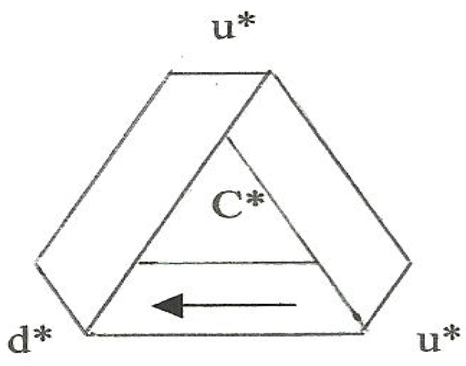


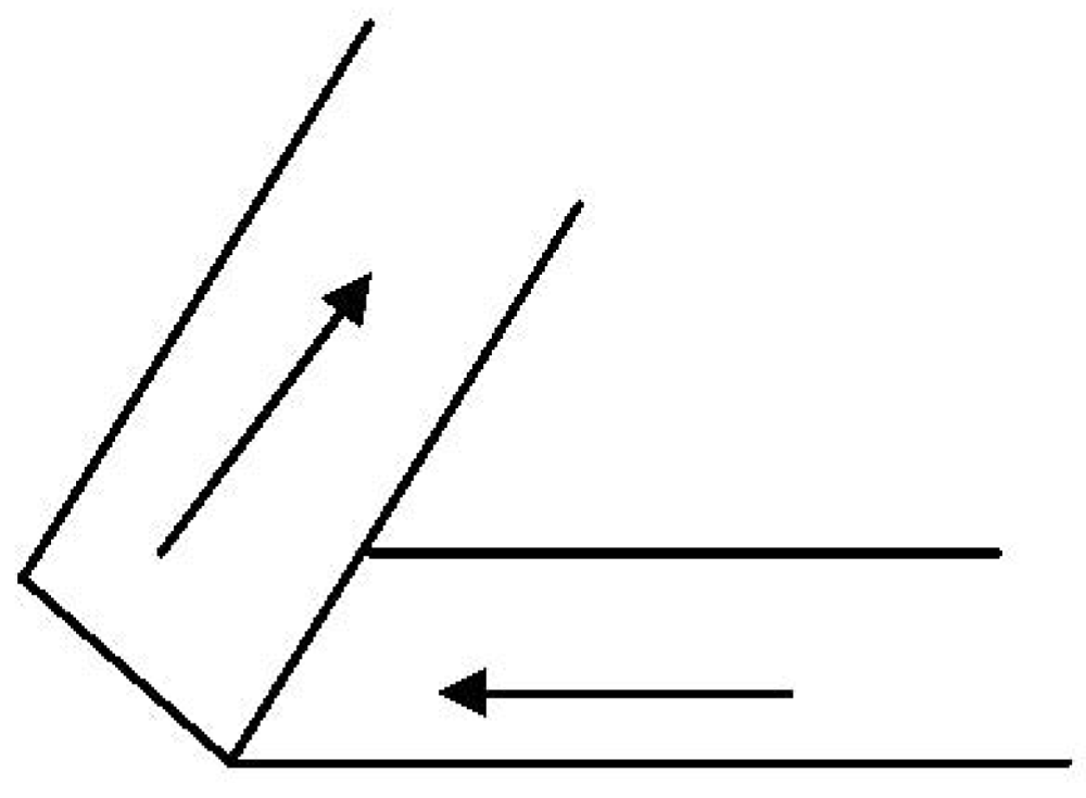
 , which fluctuates in the radial direction between the two circles of radius R − r and R + r as the particle revolves around the XY plane (the ϕ progression in our previous notation). As a result, the trajectory intersects itself such that there is an inherent ambiguity in momentum; that is, at each crossover point, the momentum is double-valued.
  to the trajectory (which is what our Equation 1-1 says) so that the rate of change of
  is unambiguous. In other words, Einstein’s (generalized) trajectory for a particle in a central field of force takes the form of a torus knot!
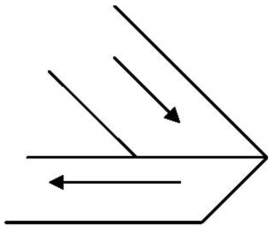
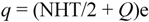


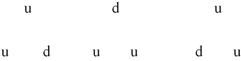


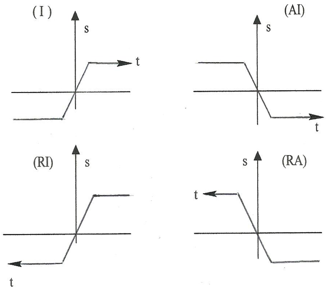
 plane (the plane of the FMS) with the
  direction normal to the plane.

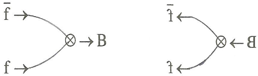
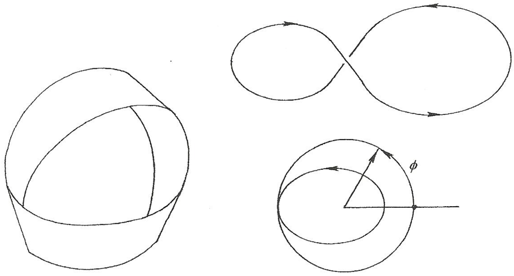

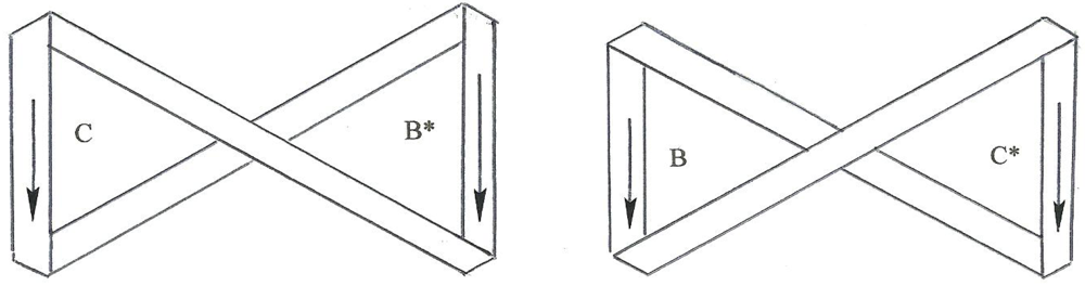

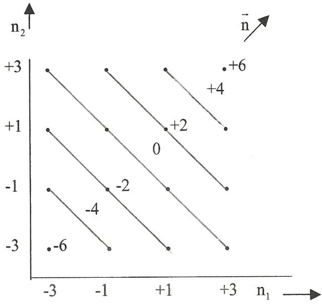
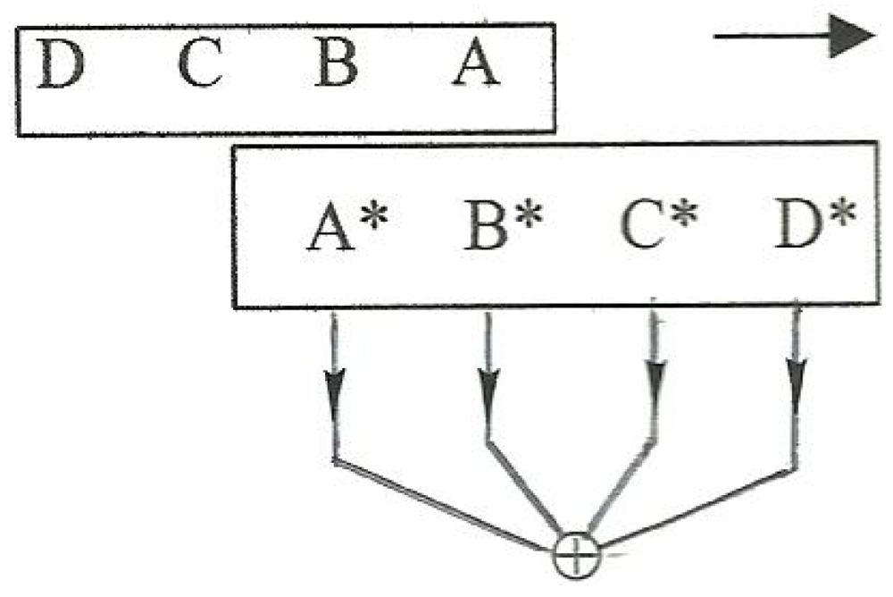


 to first order in r/R , R and r being the radii of the toroidal center line and the toroidal core, respectively andμ = n/m. The solution, well known to describe solitonic behavior (cf.[13]) is
 and is expected to be quite small.


 represent fermions and antifermions, also members of vector spaces V and V*, respectively, and the Bs are bosons, members of a certain matrix, M. One requirement for relating our model to a Hopf algebra is therefore to model the fusion and fission operations in a tensor formalism. As carried out in [2] that task is summarized in Appendix C with the result that fusion and fission can, indeed, be recognized as manifestations of the Hopf algebra operations of multiplication and comultiplication, respectively.


 ,
,  being the radial frequency and momentum eigenvector, respectively, which implies the equivalent form


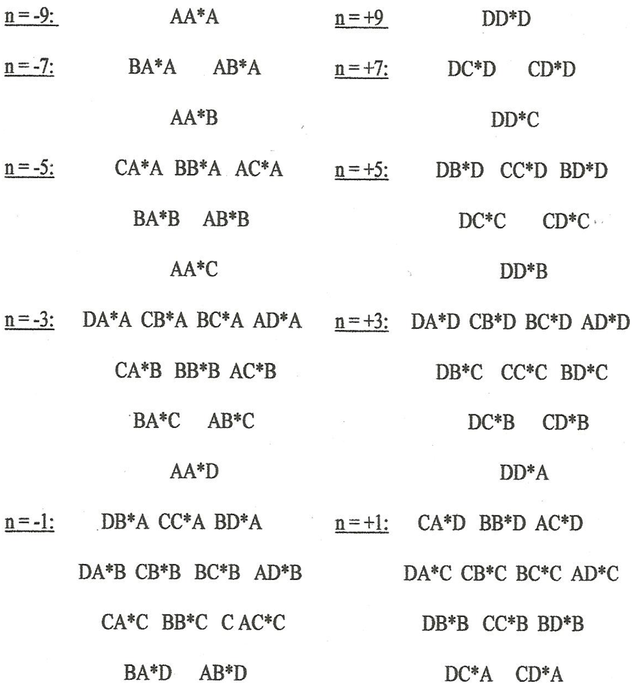


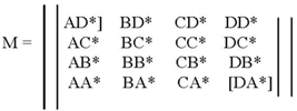

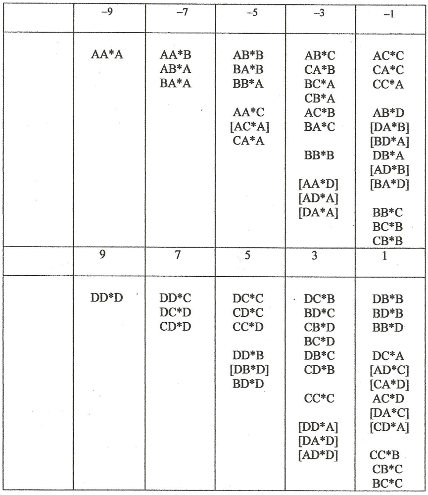


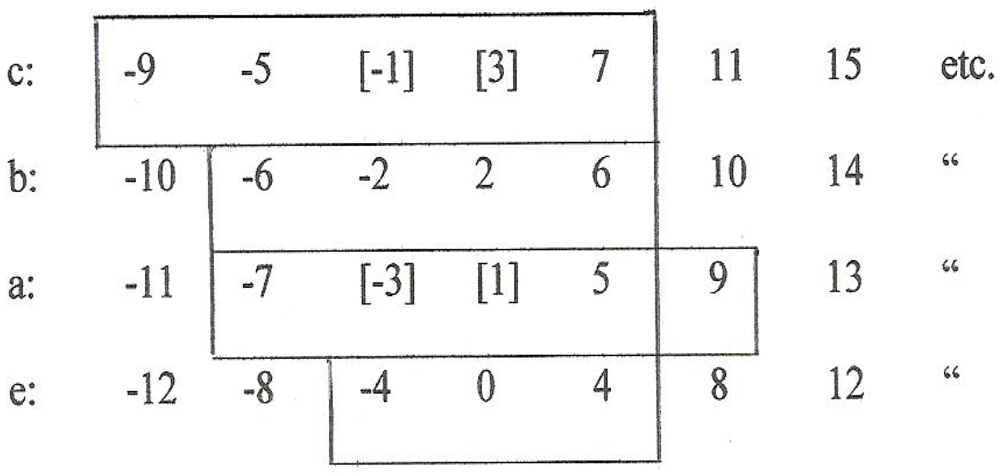


 , with k = A, B, C, or D


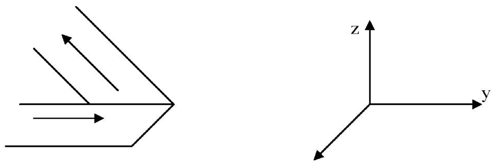
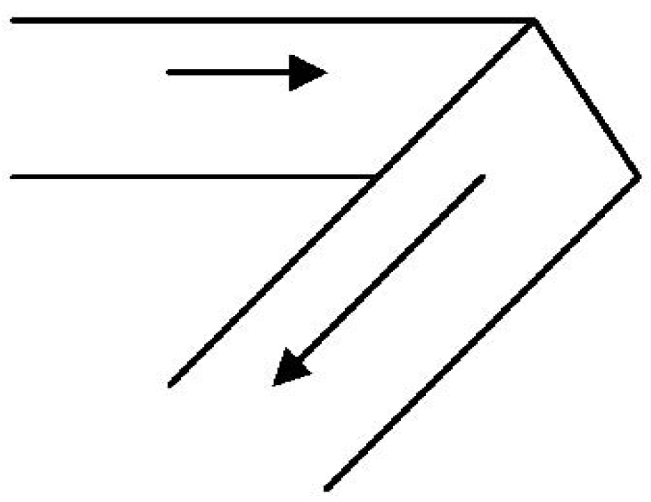
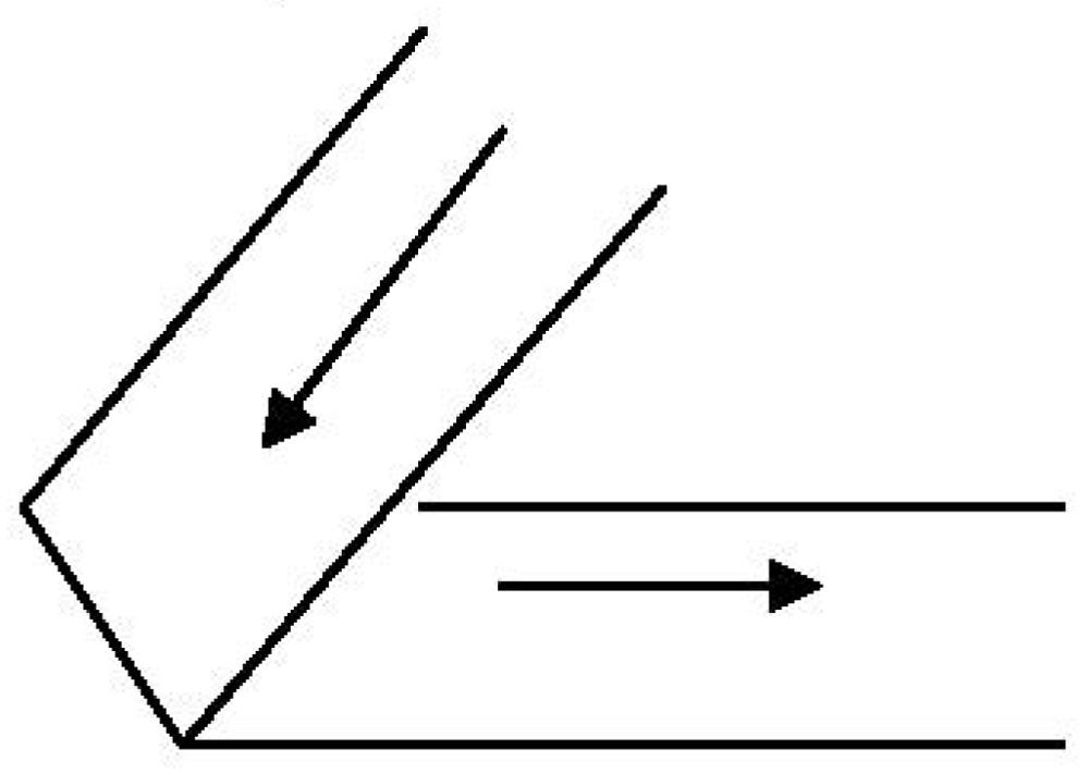
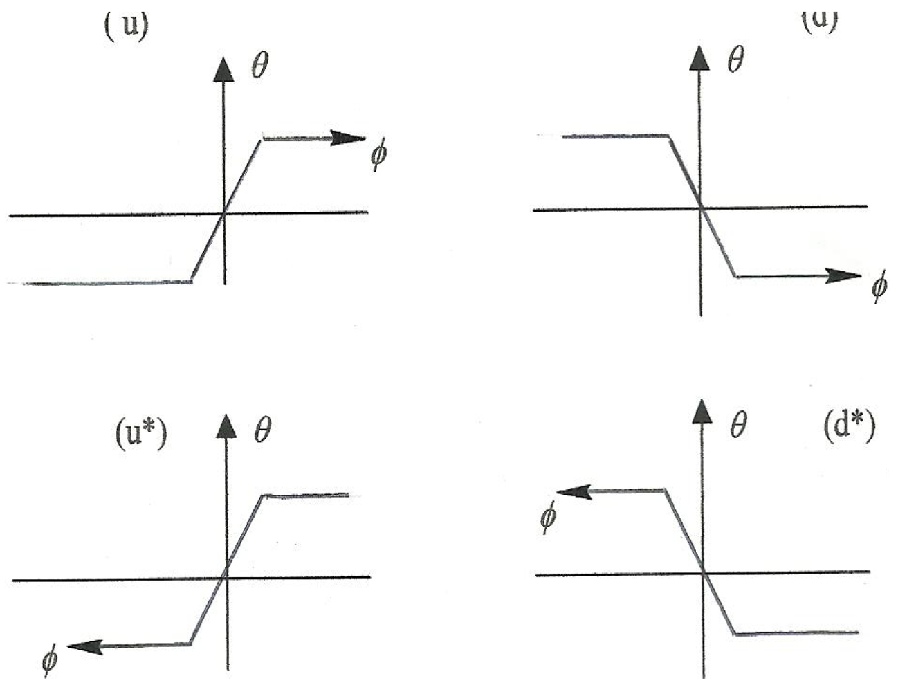
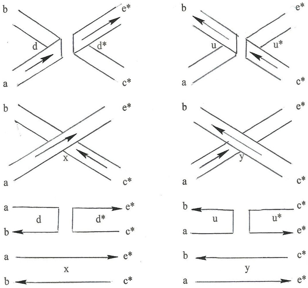
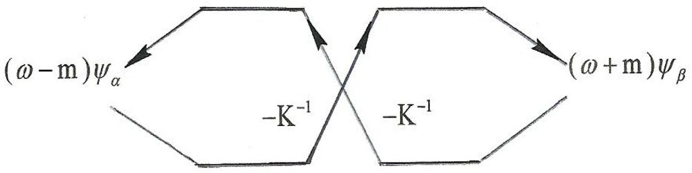
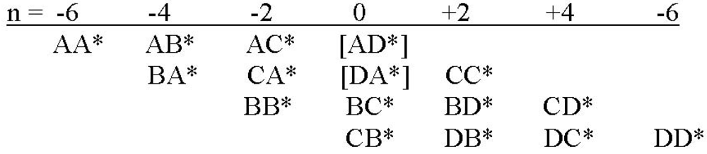
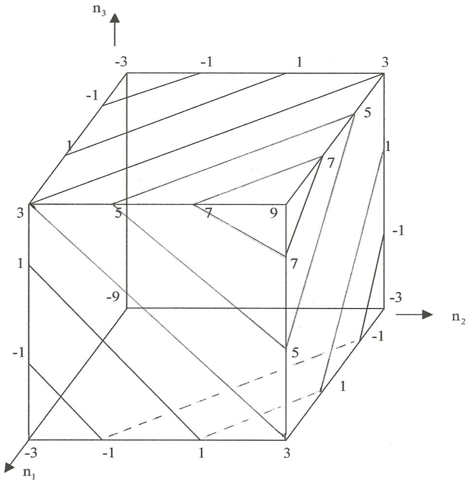
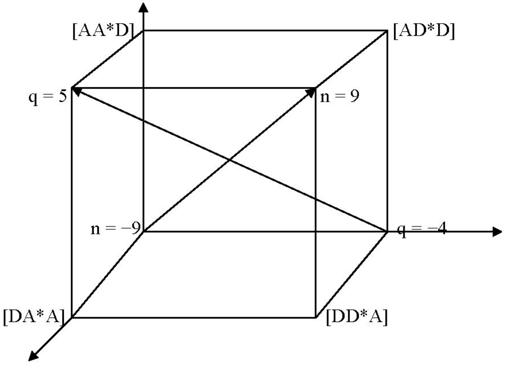
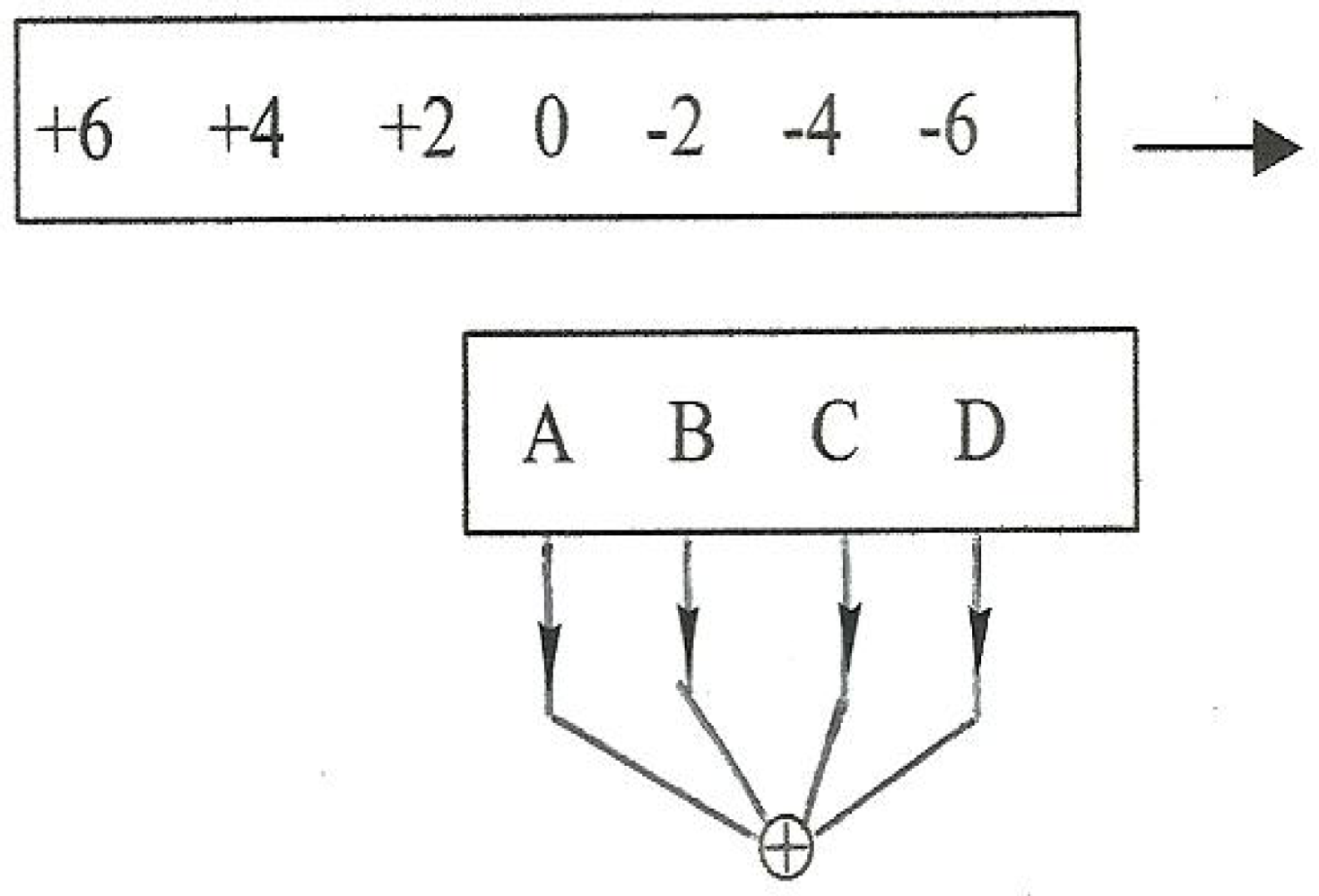
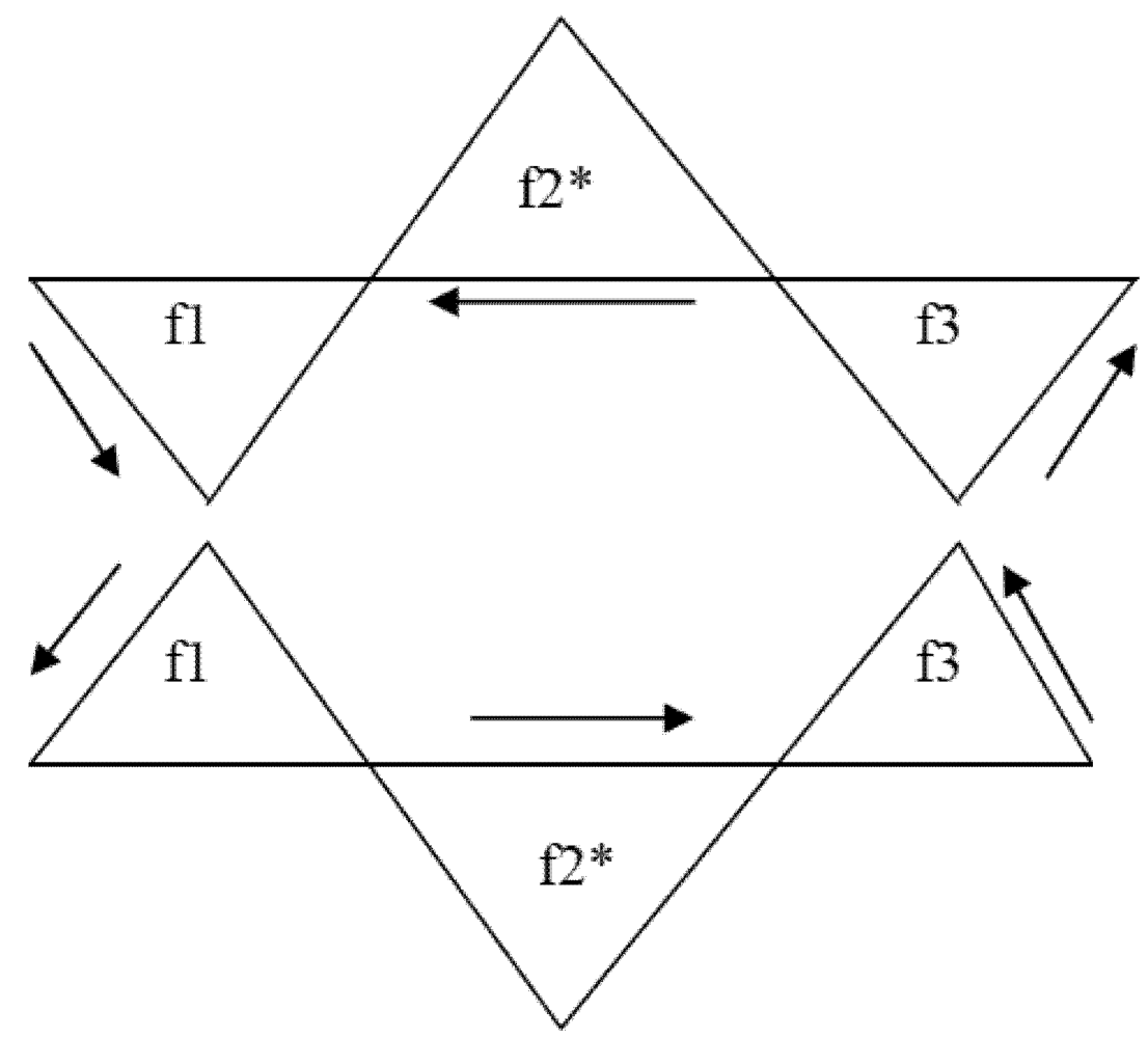
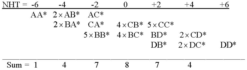
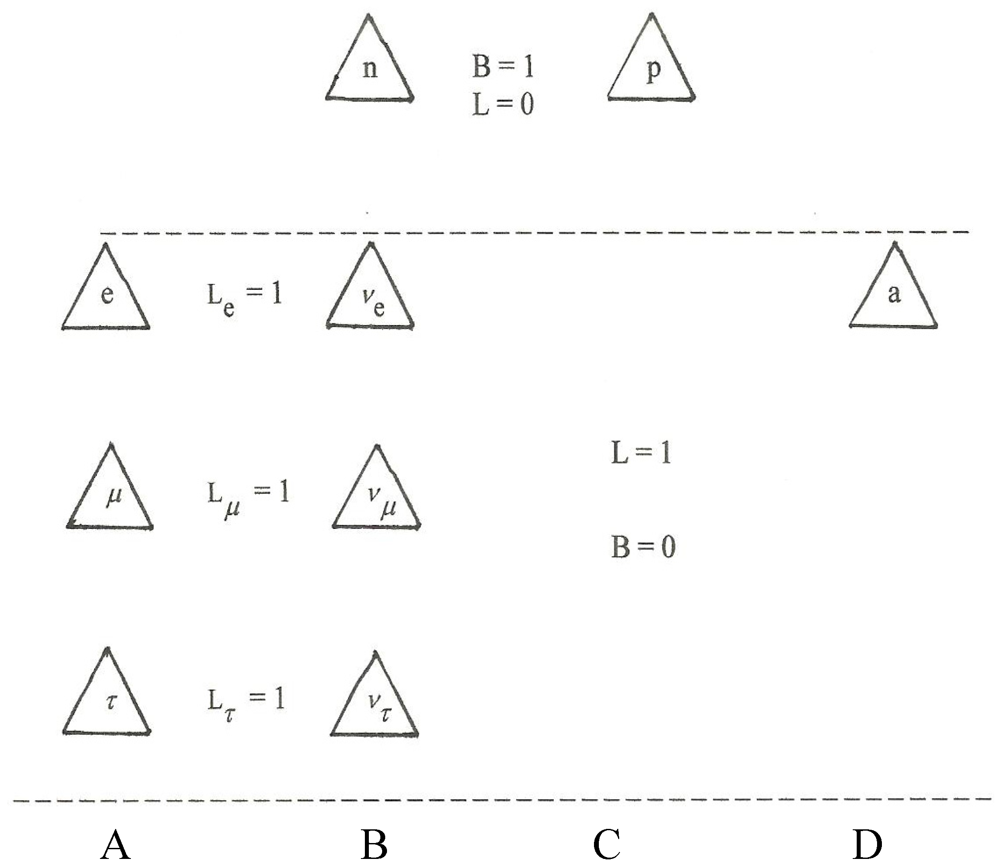
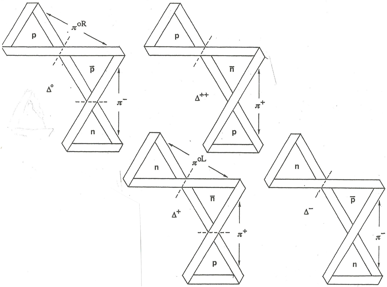
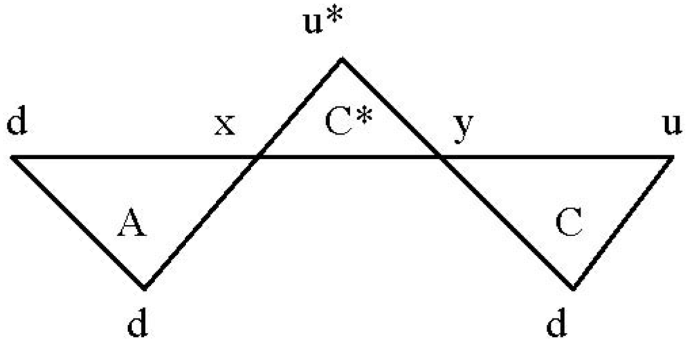
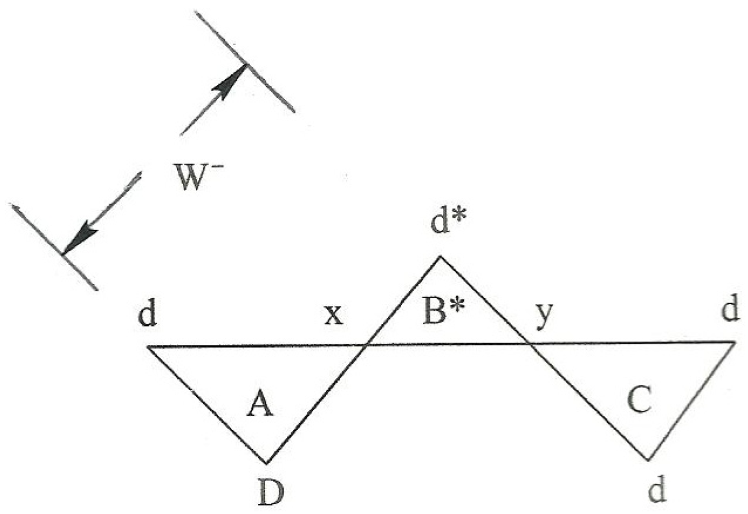
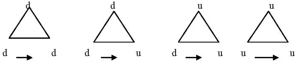
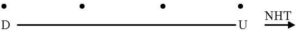
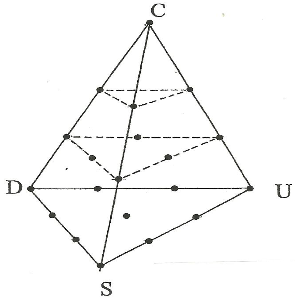
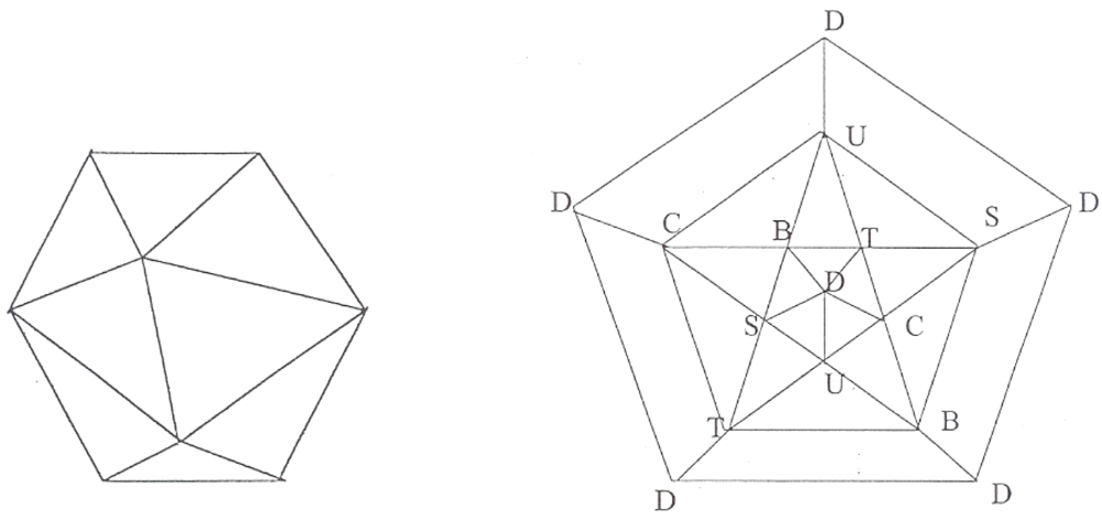
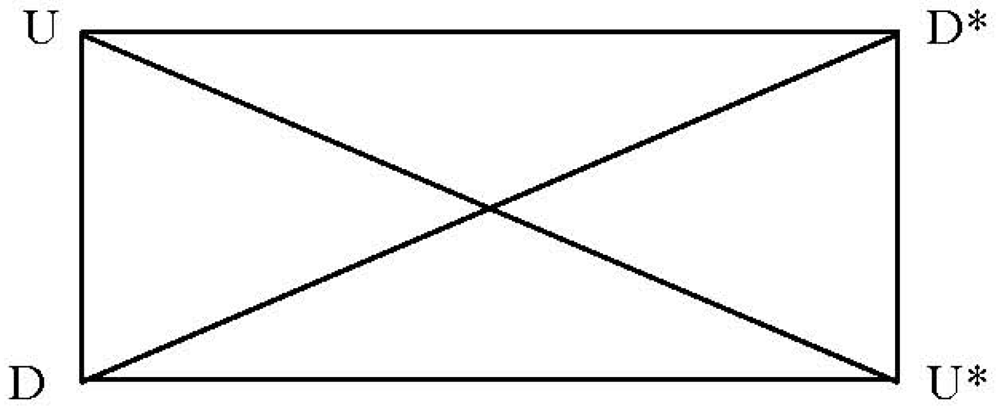
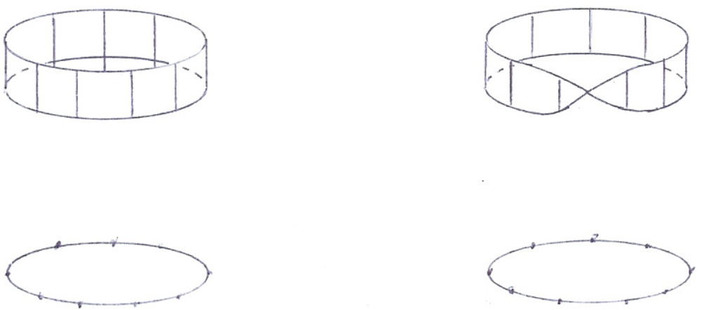
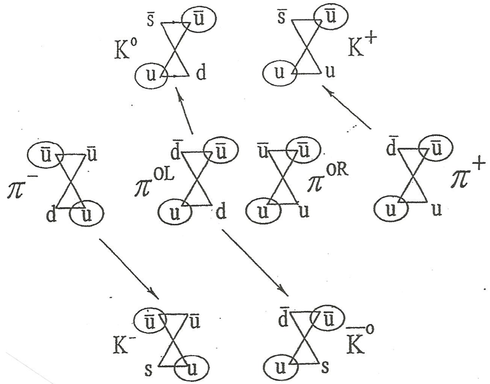
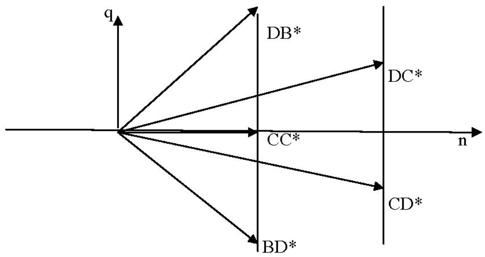
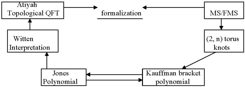
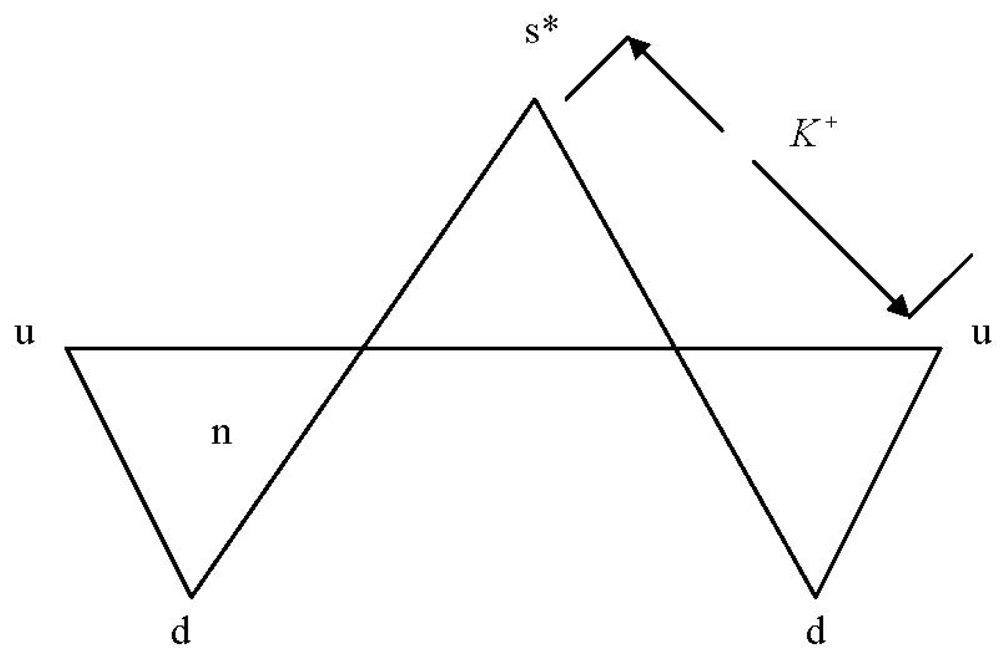
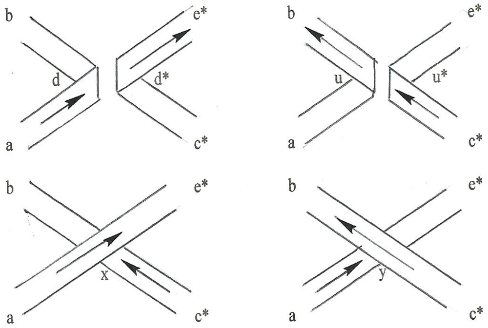
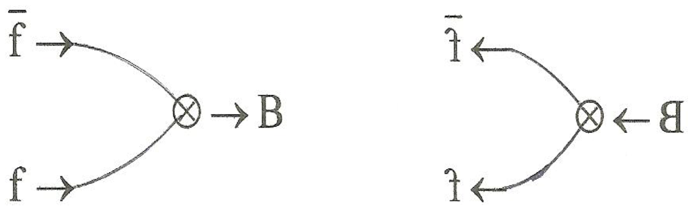
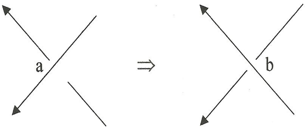
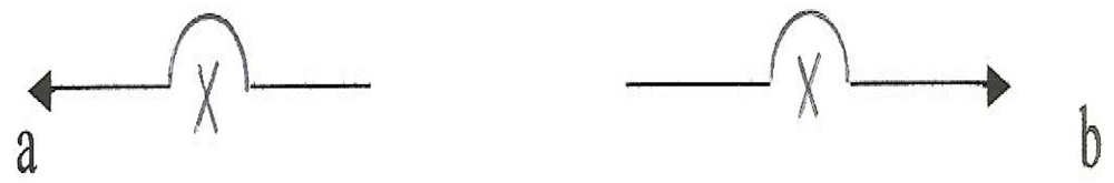
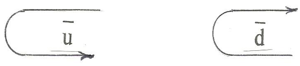
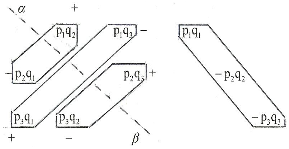
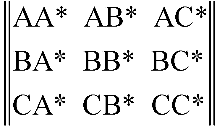
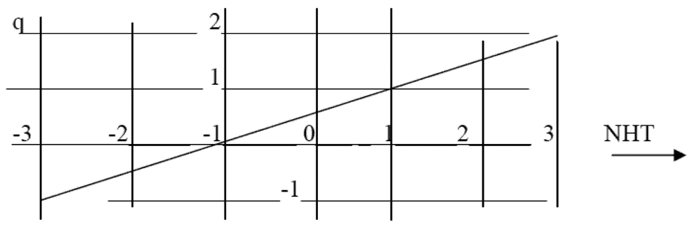
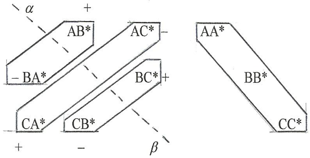
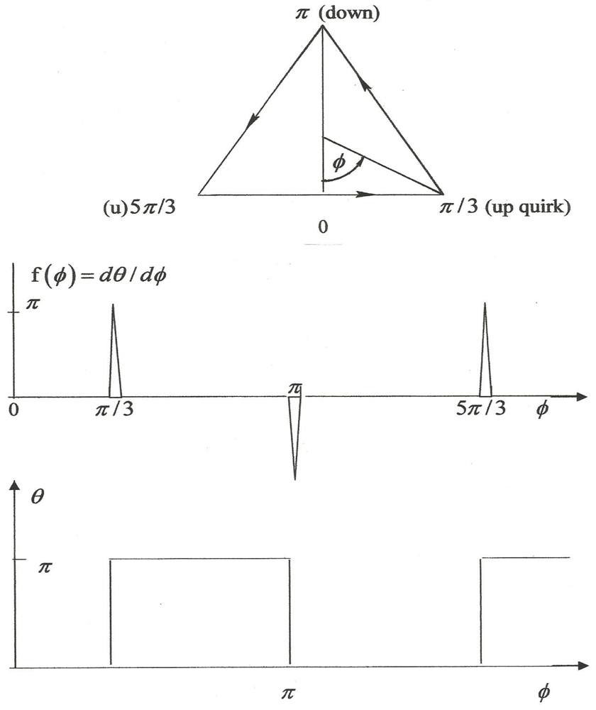


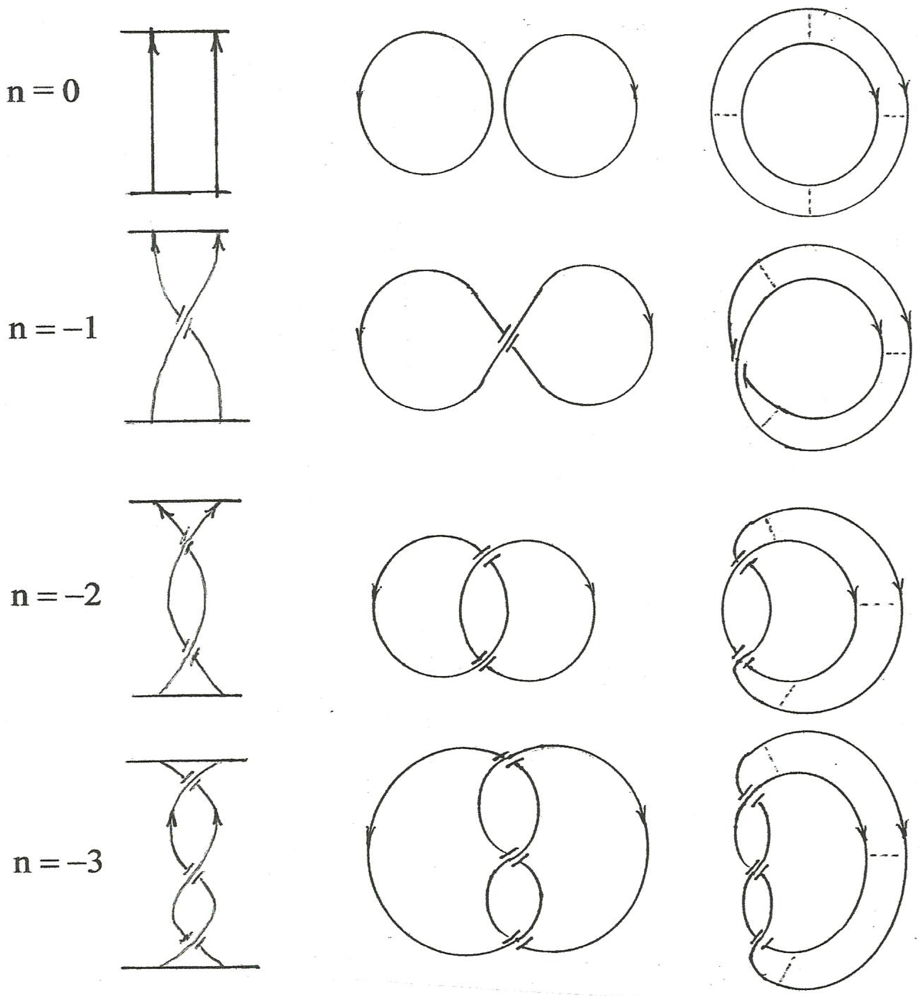


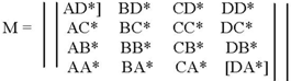


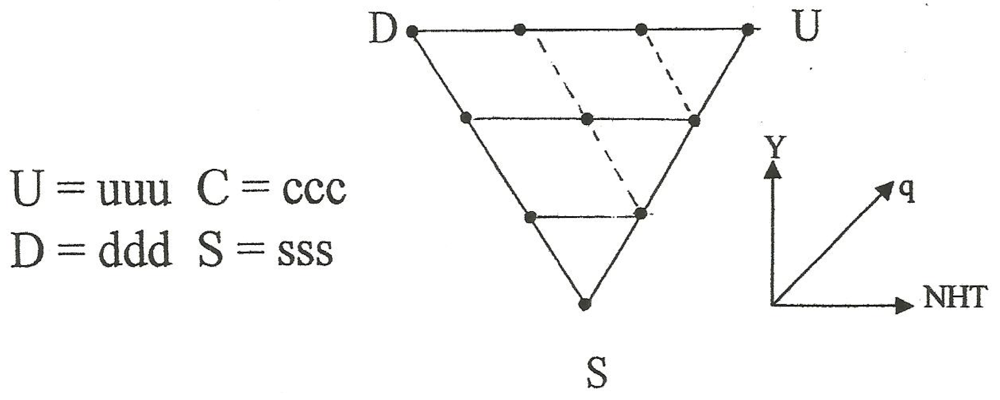
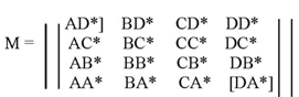


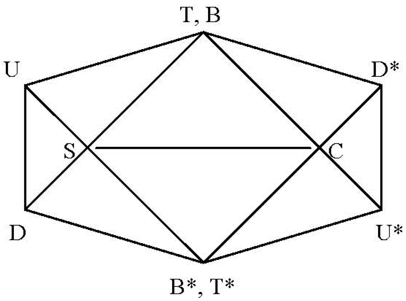


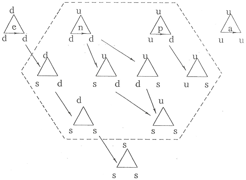
 and diagonals UU* and DD* have lengths of
  times the edge length. An example is the rectangle with edge UD connected to antipodal edge D*U* as in Figure 49.
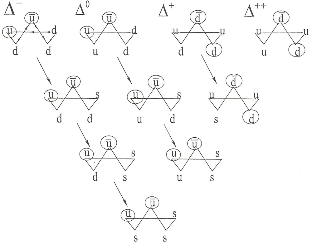

 are the normals to duads UD, TB and CS, respectively.


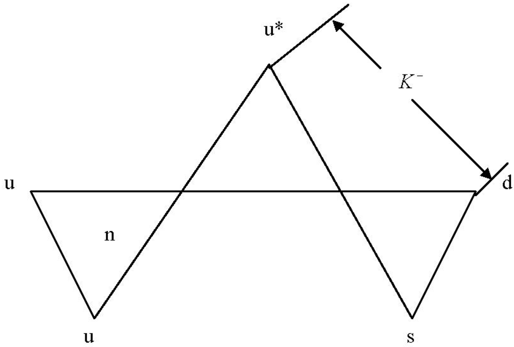


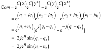


 .
.

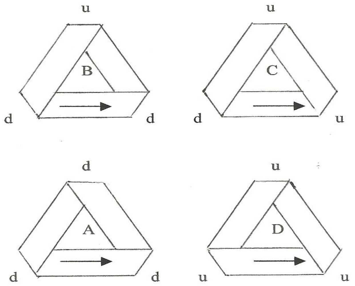


 are connection terms, in particular Christoffel symbols of the second kind, ds is the line element, and we set


 to first order in r/R.


 ,
, 


 , (differentiation is expressed by the prime superscript herein), invoke Equation (A-17) again and differentiate once more. Simplifying and rearranging then yields the desired result:


 . Then, computing applicable derivatives of this behavior (as sketched above to verify the validity of the solution to the Sine Gordon equation) we find that this modified behavior is the solution to a modified Sine-Gordon equation, namely


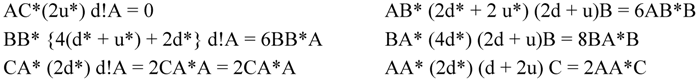


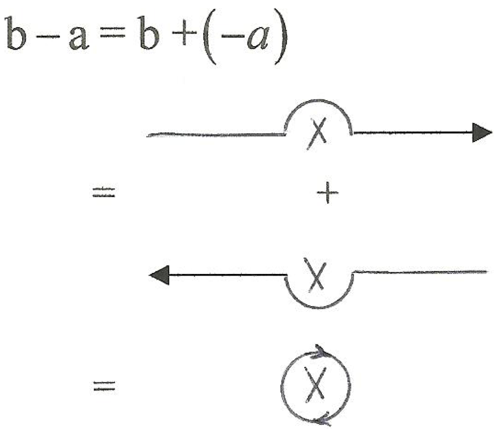


 . That development begins by identifying a 2X2 matrix
  , defined such that
  where
where  is the defining invariant for the “quantum group” and A, which appears, as below, in the well-known bracket solution to the Yang-Baxter equation, namely
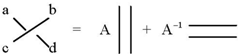
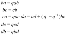
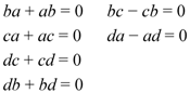


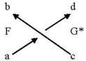
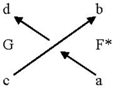

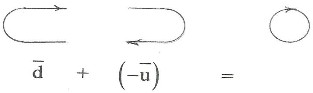
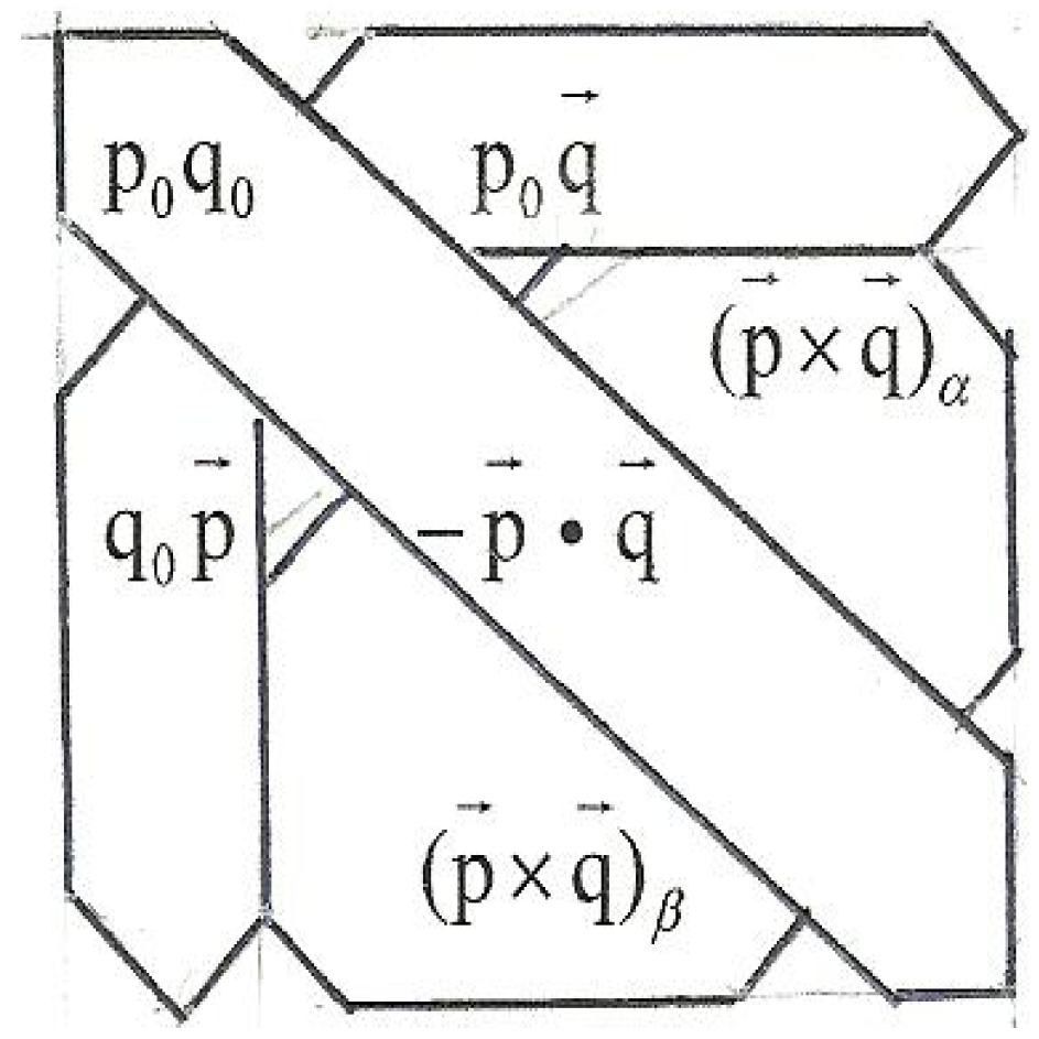


 and
and  .
.
 and
and  .
. =
= 


 or alternatively, the direct sum of the inner product and cross product of the vectors shown in Figure E2. We also note that, from the quaternion point of view, vectors

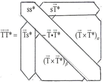


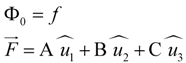
 's being isomorphic to the λs. We remark that the unit quaternion is isomorphic to the gauge group SU(2) with the unit vectors being isomorphic to the Pauli matrices.
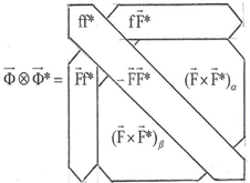
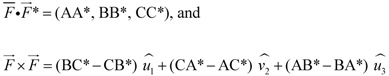
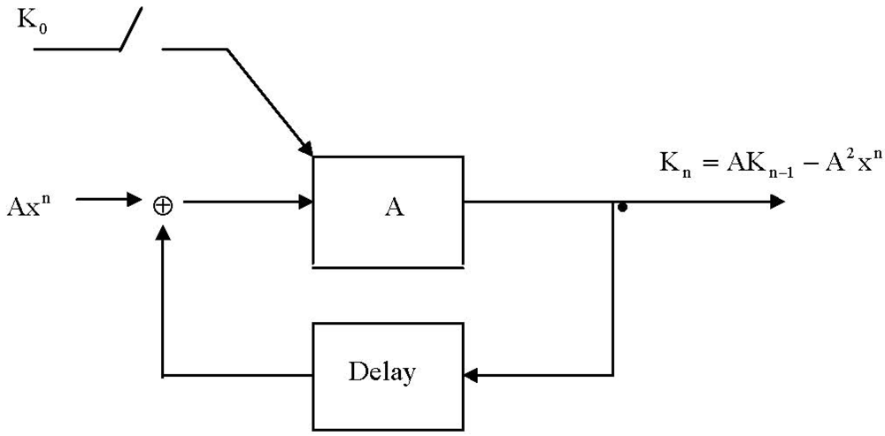

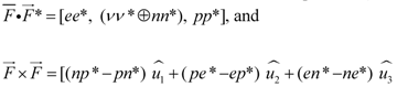
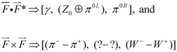

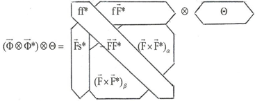
 and
and 
 ,
,  .
.


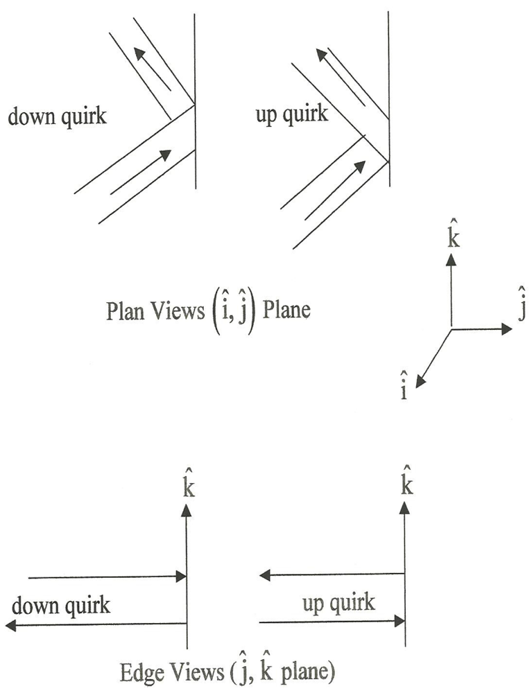


 .
.