Symmetry Groups for the Decomposition of Reversible Computers, Quantum Computers, and Computers in between

1
Department of Electronics and Information Systems, Universiteit Gent, Sint Pietersnieuwstraat 41, B-9000 Gent, Belgium
2
“FWO-Vlaanderen” post-doctoral fellow, Department of Physics and Astronomy, Universiteit Gent, Proeftuinstraat 86, B-9000 Gent, Belgium
*
Author to whom correspondence should be addressed.
Symmetry 2011, 3(2), 305-324; https://doi.org/10.3390/sym3020305
Submission received: 11 January 2011
/
Revised: 24 May 2011
/
Accepted: 27 May 2011
/
Published: 7 June 2011
(This article belongs to the Special Issue Symmetry in Theoretical Computer Science)
Abstract
:Whereas quantum computing circuits follow the symmetries of the unitary Lie group, classical reversible computation circuits follow the symmetries of a finite group, i.e., the symmetric group. We confront the decomposition of an arbitrary classical reversible circuit with w bits and the decomposition of an arbitrary quantum circuit with w qubits. Both decompositions use the control gate as building block, i.e., a circuit transforming only one (qu)bit, the transformation being controlled by the other (qu)bits. We explain why the former circuit can be decomposed into control gates, whereas the latter circuit needs control gates. We investigate whether computer circuits, not based on the full unitary group but instead on a subgroup of the unitary group, may be decomposable either into or into control gates.
1. Introduction
Quantum computing has witnessed considerable attention in the literature in the past decennia, mainly due to the speed-up of quantum computations over their classical counterparts [1,2,3]. However, an aspect that is commonly tacitly referred to the background, is the reversible character of the quantum mechanical processes, underlying the computations. Nevertheless, reversible computing offers the one-and-only road towards zero-power computation. This is due to the avoidance of the Landauer effect [4,5], i.e., no heat is dissipated into the system as no information has been destroyed along the process. Reversibility is not monopolized by the quantum world. Also classical circuits can be designed such that no information is destroyed during the computations, which constitutes the field of (classical) reversible computing [6,7,8,9,10]. These circuits are very similar to common classical logical circuits, with the exception that they are reversible, i.e., we can unambiguously reconstruct the input from any given output. An overview of the achievements in the field of reversible computation is given by Kerntopf [11]. Clearly, the set of classical reversible circuits can be regarded as a subset of the quantum reversible circuits, so classical reversible computing can be regarded as a step-up from the contemporary classical computers towards the development of the quantum computers of the future.
In the present paper, we compare the decomposition of both an arbitrary reversible circuit and an arbitrary quantum circuit into elementary gates. A relationship between the two architectures is established, based on group theory. Whereas reversible computing is based on finite groups, quantum computing is based on infinite groups (a.k.a. Lie groups). Whereas reversible computing reflects the symmetries of the group of permutation matrices, quantum computing displays the symmetries of unitary matrices. In spite of these differences, quite similar (but not identical) synthesis methods may be applied for both building a reversible computer and building a quantum computer from elementary gates called control circuits.
2. Control Circuits and Control Gates
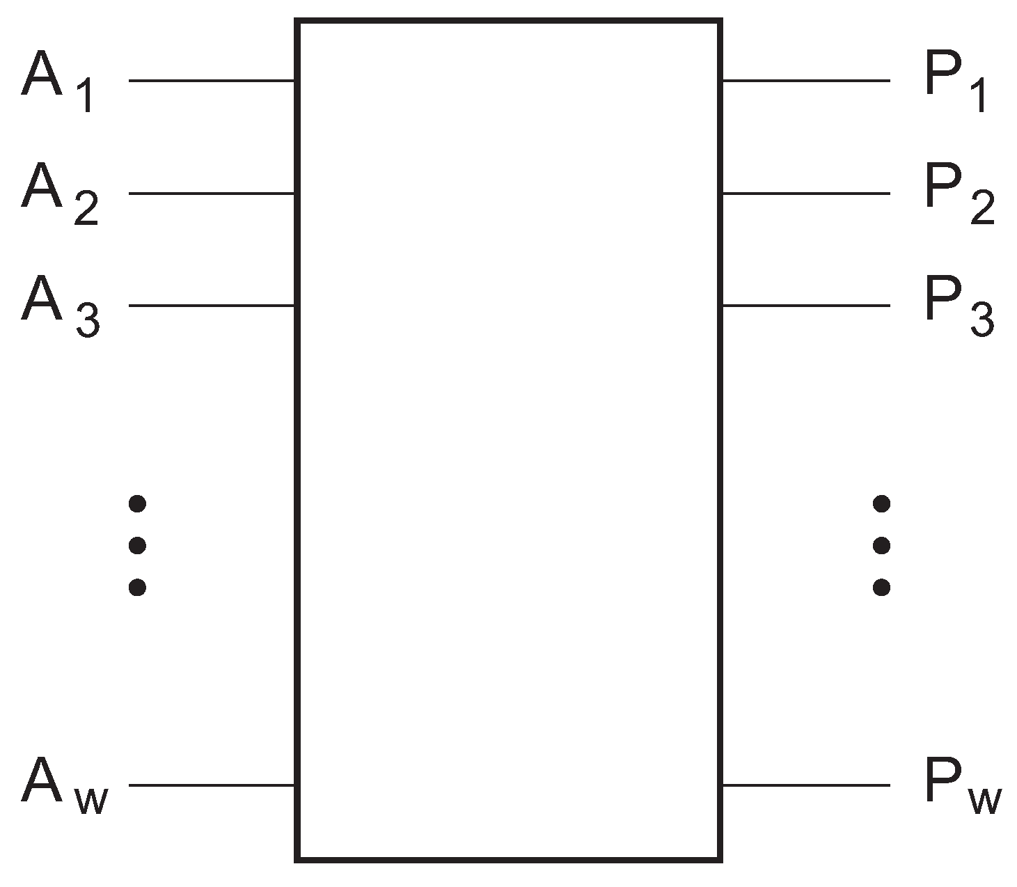
Assume a circuit of width w, i.e., a circuit with w input (qu)bits and w output (qu)bits. Indeed, for reversible circuits (either classical or quantum), the number of outputs necessarily equals the number of inputs. See Figure 1. With these w (qu)bits, we can build a dimensional (Hilbert) space with basis vectors . For a typical classical reversible circuit, the input and output vector will be equal to one of these basis vectors and we can write them as and respectively. In the quantum world, the situation is different as superpositions or linear combinations of the basis vectors (a.k.a. basis states) are part of the physical reality. So, a general state can be written as
Both in the classical case and in the quantum-mechanical case, we can represent a given (qu)bit state by means of a dimensional column vector with the coefficients (or amplitudes) as input entries. Consequently, a circuit or computation bringing one vector to another can be represented by a matrix, acting on the column vectors. These matrices are permutation matrices in the case of classical reversible computing, and become unitary matrices in the quantum case. In the classical case, the circuit is fully characterized by w Boolean functions . Methods have been developed to synthesize both circuits performing arbitrary reversible functions [9,10] and symmetric reversible functions [12].
We consider a special case of circuits, where . Let the circuit be such that it leaves the structure of the first u (qu)bits in the input state unaltered [13]. We will call these (qu)bits the controlling (qu)bits. The remaining v (qu)bits will be affected by the computation, however depending on the structure of the controlling (qu)bits. In the case of classical reversible computing, it means that the first u output bits will be equal to the input bits and the value of the remaining bits is a function of the input bits , however depending on the values of the controlling bits . In the case of quantum computing, the circuit is based on the same general principle. However, the control does not consist of the sequence alone, since the input state can be in a superposition of all basis states (1). As a result, the controlling will be done proportional to the amplitudes (with ) in the expansion of the input state. This will become clear when inspecting the transformation matrix. In general, these circuits can be represented by a matrix, consisting of blocks, each of size , situated on the diagonal. Similarly, all matrices involved are either permutation matrices (classical reversible computing) or unitary matrices (quantum computing). We will call these circuits control circuits, e.g., for the case and (and thus ), the unitary matrix looks like
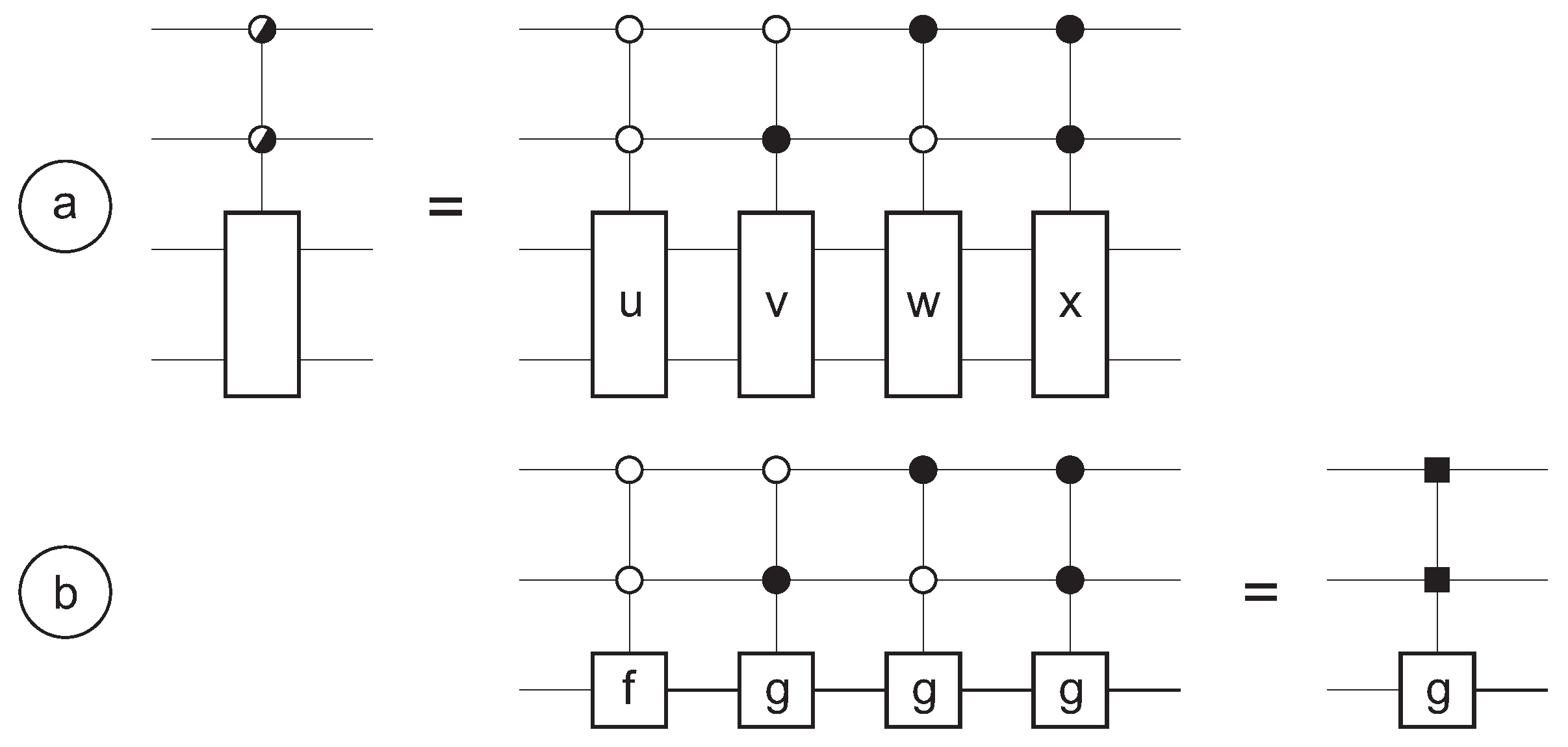
Thus, if then matrix U is applied to , if then matrix V is applied to , etc. As already mentioned, in quantum computing, the input state will always be in a superposition of the controlling qubits. Therefore, the computation will be controlled according to the amplitudes of the controlling qubits in the input state. Figure 2a shows an example for (and thus ). We follow here the notation by Möttönen et al. [14,15].
In some cases, only two different submatrices F and G are present, and moreover one of them (i.e., F) is the unit matrix. Figure 2b shows an example:
In such case, the gate g of width v is applied to the controlled (qu)bits if and only if a particular boolean function of the controlling (qu)bits equals 1. Such special control circuit is called a control gate [16]. The function is called the control function. In the example of Figure 2b, we have .
Control gates are important in classical reversible computing as there exist only two different permutation matrices, one representing the follower, the other representing the inverter. Thus a classical reversible control circuit with always simplifies to a control gate. In quantum computing, even for v as small as 1, as many as different unitary matrices [17] are allowed; the “probability” that two such blocks in a control circuit matrix will be identical, is infinitesimally small. In the following, we will show from quite general principles that the control circuit plays an important role in the effective decomposition of a reversible as well as a quantum circuit.
3. Symmetric Groups
For the study of reversible computers, we consider the reversible logic circuits of width w, i.e., with w binary inputs , , …, and w binary outputs , , …, . See Figure 1. The output rows of the truth table of such a logic transformation correspond to a permutation of the input rows (0, 0, …, 0, 0), (0, 0, …, 0, 1), (0, 0, …, 1, 0), …, and (1, 1, …, 1, 1). Table 1a gives an example for . All reversible truth tables of the same width w form a group (with respect to the operation of cascading), which we denote by R. The group R is isomorphic to the symmetric group S of degree and order . It thus is also isomorphic to the group of the permutation matrices.
A natural question is now if we can construct a given reversible function of degree x from a concatenation of circuits with lower degree. Let be the number of different circuits of degree x, which we would like to build into hardware. We may assume that we can make use of a library of circuits with degree y (with ) for that particular purpose. This library again can be constructed from another library of circuits with lower degree z (with ) etc., until we have reached the set of all circuits of degree 2 (i.e., the 1-(qu)bit operations). We are interested in a particular kind of decomposition of a circuit with a given (non-prime) degree m:
with p and q integers. We aim at decomposing a circuit of degree m into a cascade of three circuits:
- the first consisting of q subcircuits each of degree p,
- the second consisting of p subcircuits each of degree q, and
- the third consisting again of q subcircuits each of degree p.
With the help of circuits of degree p and p circuits of degree q, we can make the following number of combinations:
For the particular case of the symmetric group S of degree x, the order equals . With and , Equation (3) gives
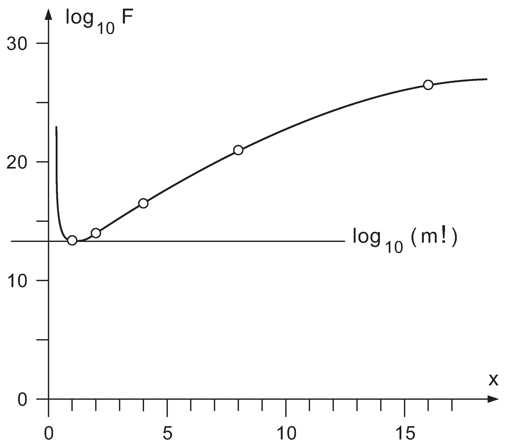
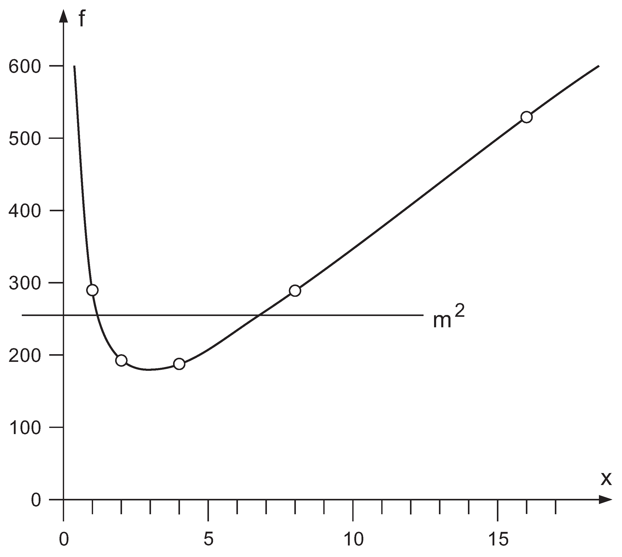
For any non-trivial divisor p of m, we have that is larger than . A proof is supplied in Appendix A. This suggests that any factorization of m is a candidate for decomposition of an arbitrary circuit of degree m, e.g., for m equal to a power of 2 (say ), we have . The value of grows fast with increasing p:
This is illustrated by Figure 3, where m has been chosen equal to 16. The dots on the curve are located at the divisors of m, i.e., at , , , , and . Thus all divisors , , …, obey . Therefore, the combinations may be enough to construct the different circuits. Hence, each of these choices of p may lead to a circuit synthesis method. And, in fact, they do, thanks to Birkhoff’s theorem on doubly stochastic matrices. One of the versions of this theorem states that any matrix with integer entries, such that all line sums are equal to p, can be written as a sum of p permutation matrices. As a result [16,18], any permutation of m objects can be decomposed as a sequence of q permutations of p objects, p permutations of q objects, and again q permutations of p objects. The most efficient synthesis method is found for that particular value of p for which exceeds as little as possible. This happens for (and thus ).
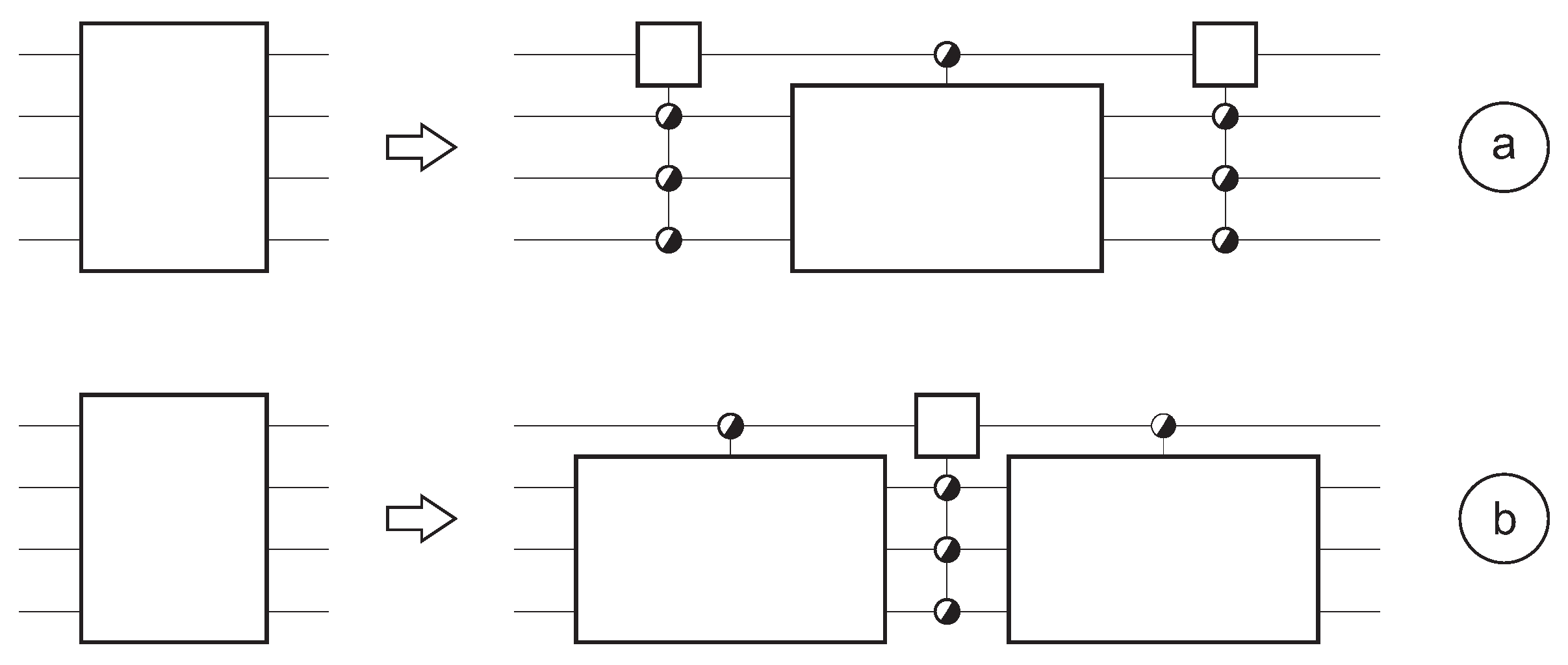
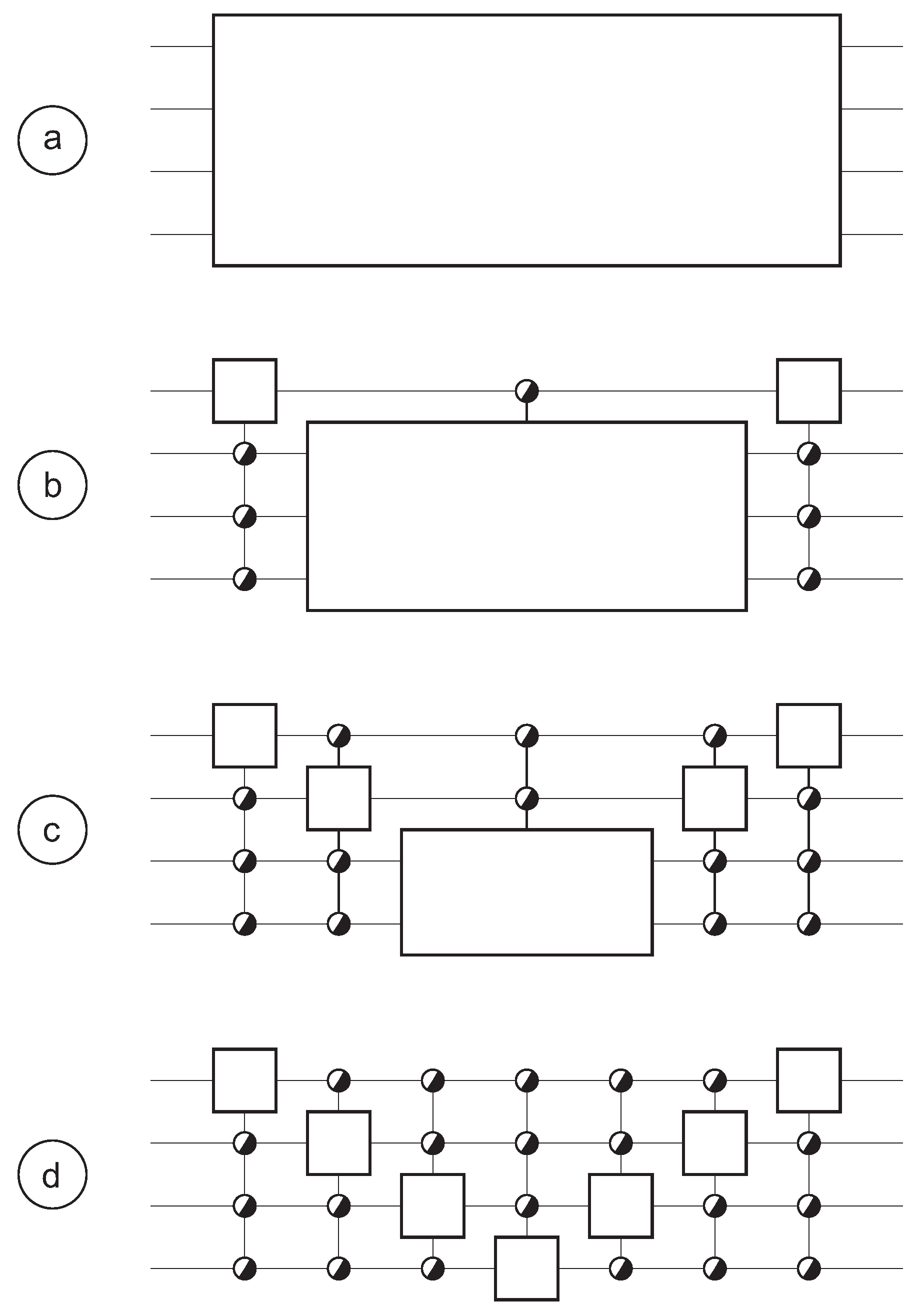
In the case of reversible computing, we have . Thus factorizing this number as is the best choice for efficient synthesis of a reversible circuit. Figure 4a shows the resulting 3-part circuit. Figure 5 shows how we may apply such decomposition times. De Vos and Van Rentergem [16,18] have demonstrated that this eventually leads to a circuit synthesis consisting of a cascade or chain of as little as control gates. The synthesis approach is very efficient, as no synthesis is possible with less than control gates. Indeed, any synthesis method [18,19] leads to a cascade of length L satisfying
with and (the number of different building blocks). Together with Stirling’s formula, this yields [18]
4. Unitary Groups
4.1. Dimensional Analysis
Let be the dimension of the space of circuits of degree x. With the help of circuits of degree p and p circuits of degree q, we can span a space of dimension
For the particular case of the unitary group U(x), the dimension equals . With and , Equation (4) gives
For most non-trivial divisors of m, we have that is smaller than . Indeed, in the range , the function first is decreasing (in the range ), then is increasing (in the range ). This is illustrated by Figure 6, where again m has been chosen equal to 16 and dots on the curve are located at the divisors of 16. The curve, in fact, is just a hyperbola. It can be noted from Figure 6 that three and only three dots are located above the horizontal line : the points at , , and . Only the point hints at a plausible decomposition, as both and do not lead towards a simplification of the original circuit. For all x-values in the range of interest (i.e., for ), is smaller than , except in the range , e.g., for m equal to a power of 2 (say ), we have and only one choice of p is viable in the latter range, i.e., :
Thus only the divisor may lead to a synthesis method. If such synthesis really exists, recursive application would eventually lead to a cascade of as little as control gates.
We summarize the present section applying the notion of Young subgroup. A Young subgroup of a symmetric group S is any direct-product group of the form S S S, where is a partition of the given number m:
Let this m be an even integer. Then:
- For any factorization , an arbitrary member a of the symmetric group S can be decomposed as the product , where both and are member of a same Young subgroup S and c is a member of a dual Young subgroup S.
- Only for the factorization , an arbitrary member a of the unitary group U(m) can be decomposed as the product , where both and are members of a same subgroup U and c is a member of a dual subgroup U.
4.2. Decomposition
In order to find the synthesis method of a quantum circuit, we successively decompose the U()-matrix according to Figure 7b, e.g., for , we have , , and . The first step in the series of decompositions looks as follows:
This decomposition indeed corresponds to the proposed cascading, as the L and R matrix can be regarded as the product of transformations in two different (orthogonal) -dimensional spaces. This can be made clear by introducing the identity
Similarly, M can be written as successive transformations in different orthogonal -dimensional spaces.
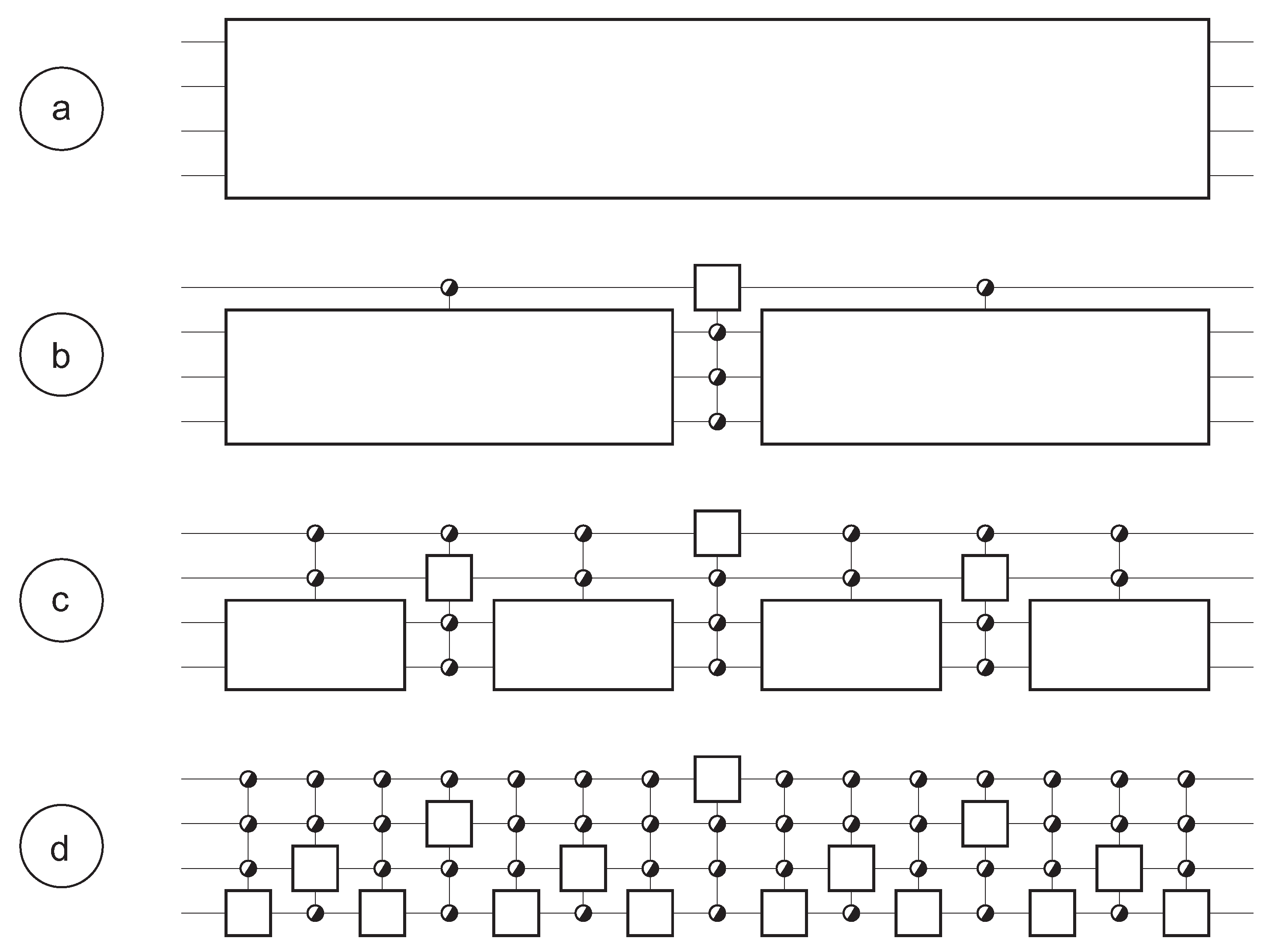
Whereas the original matrix U has parameters, the decomposition (5) has parameters, i.e., parameters for matrix L, parameters for matrix M, and parameters for matrix R. Whereas the matrix at the left-hand side of (5) is an arbitrary member of U(8), each of the three matrices at the right-hand side is member of a subgroup of U(8): two are member of a same subgroup isomorphic to U(4) and one is member of a subgroup isomorphic to U(2). Figure 4b shows the resulting 3-part circuit. Note that the matrix M represents a control circuit, however not with the wth qubit controlled, but with the first qubit controlled and the other controlling. Applying such decomposition times (Figure 7), one should be able to demonstrate that this eventually leads to a synthesis consisting of a cascade of as little as control circuits (Figure 7d).
The above synthesis approach is rather efficient, as one can prove that no synthesis is possible with less than control gates. Indeed, any synthesis method [18,19] leads to a cascades of length L satisfying
With the dimension of the total space and the dimension of each control circuits, this yields
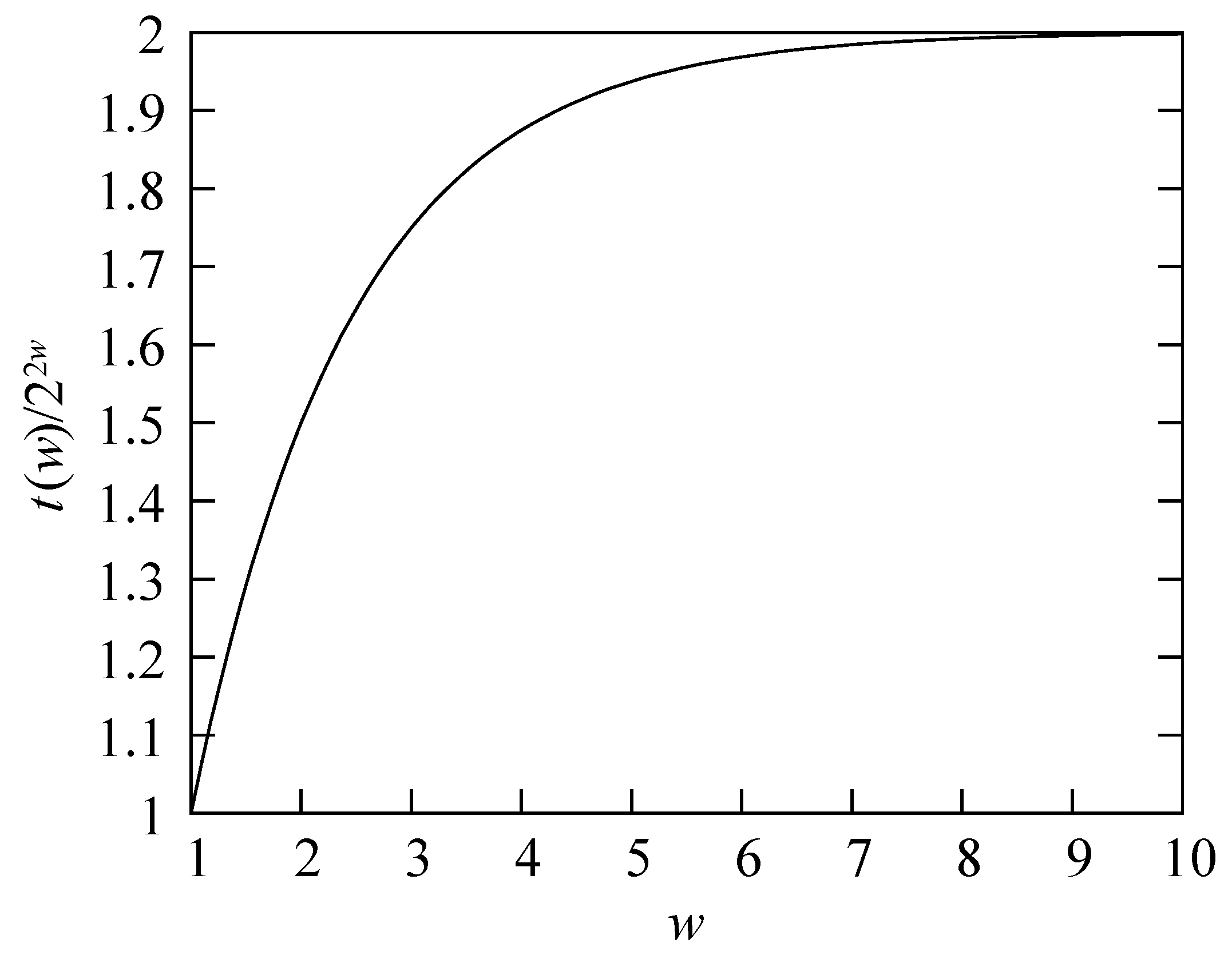
We conclude that the synthesis contains an overkill of approximately a factor 2. The reason is as follows. The decomposition (5) has parameters; therefore for only constraints, there are as many as degrees of freedom extra. In other words: after the whole decomposition is executed (Figure 7d), a total of free parameters are introduced to describe the variables of the original unitary transformation U. See Figure 8. Because of these extra degrees of freedom, we are allowed to choose a controlled ROTATOR as control circuit. Each of the blocks within the M-matrix then has the form
Such matrices form a well-known 1-dimensional subgroup of the 4-dimensional group U(2). See Appendix B. As a result, decomposition (5) is the well-known cosine-sine decomposition [20]. Of the degrees of freedom, only remain: the rotation angles , , …, . The cosine-sine decomposition has indeed been applied for quantum circuit synthesis [14,21,22,23,24].
With the cosine-sine approach, each of the blocks in Figure 7d comes from a space with dimension , except the blocks in the lowermost line, which come from a space still with dimension . Thus the total dimension is
such that there is only an overkill anymore of 5/4 with respect to the dimension of Figure 7a, instead of a factor 2.
4.3. Alternative Approaches
Möttönen et al. [14] first apply the cosine-sine decomposition (as in Section 4.2), then apply times the identity
The former factor of the right-hand side becomes a block of the M-matrix in (5); the latter factor is absorbed by the R-matrix. By clever choice of the parameters and subsequent application of a “mirroring trick”, all the blocks in Figure 7d are member of a 2-dimensional subspace of U(2). The total dimension of their final synthesis exactly matches .
Many other variations to the cosine-sine decomposition are possible, e.g., in order to obtain a decomposition of an arbitrary quantum circuit more closely resembling the decomposition of a reversible circuit (as given in Section 3), we may apply the identities
We let the first two factors of the right-hand side be absorbed by the L-matrix and the last factor by the R-matrix. This leaves the third factor of the right-hand side as a block of the M-matrix. Thus, the blocks (in the upper rows) of Figure 7d become controlled NEGATORs (See Appendix C) instead of controlled ROTATORs.
5. Intermediate Groups
The symmetric group is a subgroup of U(). As a result, any member of can obviously be decomposed by means of the cosine-sine decomposition (Figure 7). However, this is not a very cost-efficient way of proceeding because we know, by virtue of the Birkhoff theorem, that a decomposition according Figure 5 is also possible. Moreover, every elementary control gate in the latter decomposition is a member of , which also belongs to the family of symmetric groups (). From this perspective, it would be interesting to investigate whether any member of a notable subgroup X() of U() (or supergroup of ) can be decomposed into elementary control gates within the same family of those subgroups (e.g., decomposing the elements of the orthogonal group O() into multiple controlled O(2) gates). Furthermore, it is of interest to know whether such a decomposition is necessarily “cosine-sine”-like (Figure 4b & Figure 7) or may be achieved by means of a cheaper Birkhoff-like architecture (Figure 4a & Figure 5).
Consider Lie groups of matrices with dimension , not necessarily equal to (unitary matrices) or to 0 (permutation matrices). In particular, we focus on functions satisfying
which are natural assumptions when dealing with matrix groups. For convenience, we put forward the quadratic form
in accordance to the classical groups [25]. This assumption will enable us to analyze the decomposition for groups ranging in between reversible and quantum computing. In general, the basis assumptions (6) lead to
By means of the dimensional analysis performed in the previous sections, we can extract necessary (but not sufficient) conditions for a decomposition to be feasible. For both the “cosine-sine”-like and Birkhoff-like architecture, the analysis breaks down to the level of Figure 4. We obtain:
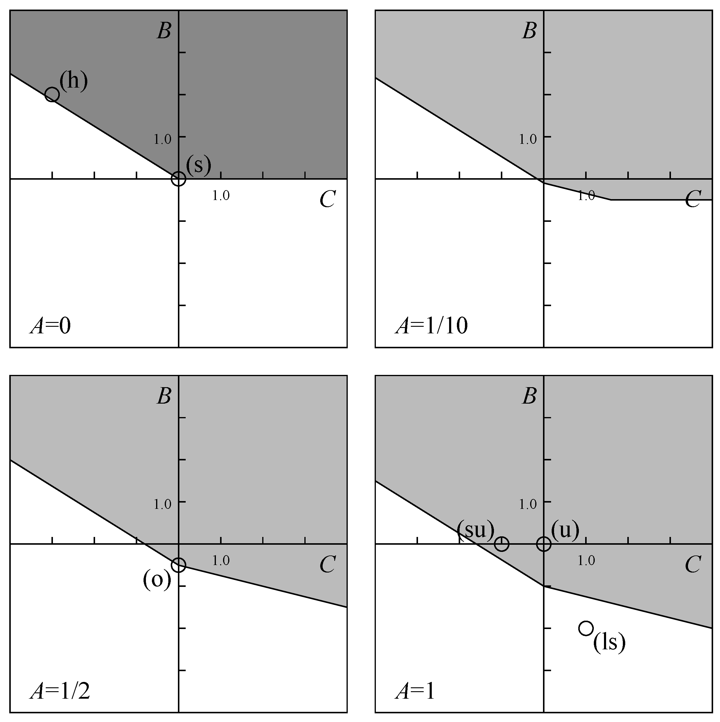
- For a decomposition like Figure 4a to be possible, it is necessary thati.e., thatSubstitution of (7) into (9) givesleading to the additional condition . This result, together with from (8) sets , such that . As a result, the necessary conditions for a decomposition according to Figure 4a (and subsequently a Birkhoff like decomposition) areThis is illustrated by the dark gray domain in the upper left panel of Figure 9. It may be noted that the conditions for a Birkhoff-like decomposition almost coincide with the general conditions (8) for . Therefore, a linear-dimensional matrix group () is likely to be decomposable by means of a Birkhoff architecture. An example would be the Heisenberg group H(), which is a linear-dimensional Lie group [26] of dimension and is depicted in the upper left panel of Figure 9 by (h). At this point, it is worth stressing that (10) is a necessary and not a sufficient condition. Therefore, once a particular group has passed the test (10), it is not guaranteed that it is Birkhoff-style decomposable. The Heisenberg group is a notable example, because deeper analysis points out that a general Heisenberg matrix of H() cannot be decomposed into a member of H H H. So, although the Heisenberg group fulfills relation (10), in general it can not be decomposed into a Birkhoff-style architecture. For quadratic groups, the conclusion we can draw from (10) is much more straightforward: since , a general Birkhoff-like decomposition is impossible on dimensional grounds.
- For a decomposition like Figure 4b to be possible, it is necessary thati.e., thatSubstitution of (7) into (11) givesleading to the additional condition . As a result, the necessary conditions for a decomposition according to Figure 4b (and subsequently a “cosine-sine”-like decomposition) areThis is illustrated by the light gray domains in the panels of Figure 9. It should be noted that, for , the conditions (10) and (12) coincide exactly. The result suggests that a large set of Lie groups may profit from a decomposition according Figure 4b. As an example, we consider the unitary matrices with all line sums equal to 1. They form a Lie group with dimension and are depicted by (ls) in Figure 9. The group is both a subgroup of U(m) and a supergroup of . Here, neither (10) nor (12) is fulfilled. Thus these matrices cannot be decomposed, neither as in Figure 4a nor as in Figure 4b, and consequently neither as in Figure 5d nor as in Figure 7d. Another example consists of the unitary matrices with only real entries. These matrices form the orthogonal group O(m) with dimension and are depicted by (o) in Figure 9. This time, (10) is not fulfilled, but (12) is, such that the Birkhoff-like decomposition is not applicable, but the “cosine-sine”-like decomposition may be applicable. As a matter of fact, it is. This is no surprise, as the cosine-sine decomposition is proved for orthogonal matrices [27]. In contrast to the general case treated in Section 4.2, the lowermost row of blocks in Figure 7d, in the orthogonal case, are member of the same O(2) group as the other blocks. The same is valid for the special unitary groups SU(m) with , depicted by (su) in Figure 9.
6. Conclusions
An arbitrary classical reversible computer can be decomposed into controlled NOT gates. In a similar way, an arbitrary quantum computer can be decomposed into control circuits (either controlled ROTATOR circuits, or controlled NEGATOR circuits, or …). Whereas the reversible circuit decomposition is based on the Birkhoff decomposition of doubly stochastic matrices, the quantum circuit decomposition is based on the cosine-sine decomposition of unitary matrices. Lie groups, other than the unitary groups, may either profit of similar decompositions or not, depending on their dimension.
References and Notes
- Shor, P. Polynomial-time algorithms for prime factorization and discrete logarithms on a quantum computer. SIAM J. Comput. 1997, 26, 1484–1509. [Google Scholar] [CrossRef]
- Grover, L. Quantum mechanics helps in searching for a needle in a haystack. Phys. Rev. Lett. 1997, 79, 325–328. [Google Scholar] [CrossRef]
- Deutsch, D.; Jozsa, R. Rapid solution of problems by quantum computation. Proc. R. Soc. London Ser. A 1992, 439, 553–558. [Google Scholar] [CrossRef]
- Landauer, R. Irreversibility and heat generation in the computational process. IBM J. Res. Dev. 1961, 5, 183–191. [Google Scholar] [CrossRef]
- Keyes, R.; Landauer, R. Minimal energy dissipation in logic. IBM J. Res. Dev. 1970, 14, 153–157. [Google Scholar] [CrossRef]
- Markov, I. An introduction to reversible circuits. In Proceedings of the 12th International Workshop on Logic and Synthesis, Laguna Beach, CA, USA, May 2003; pp. 318–319. [Google Scholar]
- De Vos, A.; Van Rentergem, Y. From group theory to reversible computers. Int. J. Unconv. Comput. 2007, 4, 79–88. [Google Scholar]
- Hayes, B. Reverse engineering. Am. Sci. 2006, 94, 107–111. [Google Scholar] [CrossRef]
- Wille, R.; Drechsler, R. Towards a Design Flow for Reversible Logic; Springer: Dordrecht, The Netherlands, 2010. [Google Scholar]
- De Vos, A. Reversible Computing; Wiley-VCH: Weinheim, Germany, 2010. [Google Scholar]
- Kerntopf, P. Research on reversible computation in the year 2010. In Proceedings of the 3rd Reversible Computation Workshop, Gent, Belgium, July 2011. [Google Scholar]
- Wille, R.; Drechsler, R. BDD-based synthesis of reversible logic for large functions. In Proceedings of the 46th Design Automation Conference, San Francisco, CA, USA, July 2009; pp. 270–275. [Google Scholar]
- Thus a measurement of these (qu)bits before or after the computation would lead to the same results.
- Möttönen, M.; Vartiainen, J.; Bergholm, V.; Salomaa, M. Quantum circuits for general multi-qubit gates. Phys. Rev. Lett. 2004, 93, 130502. [Google Scholar] [CrossRef] [PubMed]
- Bergholm, V.; Vartiainen, J.; Möttönen, M.; Salomaa, M. Quantum circuits with uniformly controlled one-qubit gates. Phys. Rev. A 2005, 71, 052330. [Google Scholar] [CrossRef]
- De Vos, A.; Van Rentergem, Y. Young subgroups for reversible computers. Adv. Math. Commun. 2008, 2, 183–200. [Google Scholar]
- Here the infinity sign ∞ refers to the cardinality of the real numbers, i.e., to an uncountable infinity. As an m × m complex matrix has m2 comples entries, there are such matrices. The unitarity condition, however, introduces m2 restrictions, leaving m2 degrees of freedom and hence such matrices.
- De Vos, A.; Van Rentergem, Y. Networks for reversible logic. In Proceedings of the 8th International Workshop on Boolean Problems, Freiberg, Germany, September 2008; pp. 41–47. [Google Scholar]
- De Vos, A.; De Baerdemacker, S. Linear reversible computing: Digital versus analog. Int. J. Unconv. Comput. 2010, 6, 239–263. [Google Scholar]
- Bhatia, R. Matrix Analysis; Springer: New York, NY, USA, 1997; pp. 195–203. [Google Scholar]
- Khan, F.; Perkowski, M. Synthesis of ternary quantum logic circuits by decomposition. In Proceedings of the 7th International Symposium on Representations and Methodology of Future Computing Technologies, Tokyo, Japan, September 2005; pp. 114–118. [Google Scholar]
- Slepoy, A. Quantum Gate Decomposition Algorithms; Sandia Report, SAND2006-3440; Sandia National Laboratories: Albuquerque, NM, USA, 2006.
- Shende, V.; Bullock, S.; Markov, I. Synthesis of quantum-logic circuits. IEEE Trans. Comput. Aided Des. Integr. Circuits Syst. 2006, 25, 1000–1010. [Google Scholar] [CrossRef]
- Nakajima, Y.; Kawano, Y.; Sekigawa, H. A new algorithm for producing quantum circuits using KAK decompositions. Quantum Inf. Comput. 2006, 6, 67–80. [Google Scholar]
- Gilmore, R. Lie Groups, Lie Algebras and Some of Their Applications; John Wiley & Sons: New York, NY, USA, 1974. [Google Scholar]
- Hall, B. Lie Groups, Lie Algebras, and Representations; Springer: New York, NY, USA, 2003; pp. 18–25. [Google Scholar]
- Golub, G.; Van Loan, C. Matrix Computations; John Hopkins University Press: Baltimore, MD, USA, 1996; pp. 75–79. [Google Scholar]
- Barenco, A.; Bennett, C.; Cleve, R.; DiVincenzo, D.; Margolus, N.; Shor, P.; Sleator, T.; Smolin, J.; Weinfurter, H. Elementary gates for quantum computation. Phys. Rev. A 1995, 52, 3457–3467. [Google Scholar] [CrossRef] [PubMed]
- Gasiorowicz, S. Quantum Physics; John Wiley: New York, NY, USA, 1974; p. 232. [Google Scholar]
- Deutsch, D. Quantum computation. Phys. World 1992, 5, 57–61. [Google Scholar] [CrossRef]
- Deutsch, D.; Ekert, A.; Lupacchini, R. Machines, logic and quantum physics. Bull. Symbolic Log. 2000, 3, 265–283. [Google Scholar] [CrossRef]
- Galindo, A.; Martín-Delgado, M. Information and computation: Classical and quantum aspects. Rev. Mod. Phys. 2002, 74, 347–423. [Google Scholar] [CrossRef]
- Miller, D. Decision diagram techniques for reversible and quantum circuits. In Proceedings of the 8th International Workshop on Boolean Problems, Freiberg, Germany, September 2008; pp. 1–15. [Google Scholar]
Appendix
A. Proof of a Theorem in Combinatorics
We assume p and q are integers, satisfying and . We prove that
by induction in q:
A1. The hypothesis holds for , because is larger than .
A2. We assume that (13) holds for . Then:
such that (13) also holds for . Note that in the ≥ step above, we have taken advantage of the property that . This, in turn, is a consequence of
where all p factors of the right-hand side (except the first one and the last one) are larger than p.
A3. Because of A1 and A2, the hypothesis is true for all .
B. Lie Algebra of U(2)
An arbitrary matrix with complex entries has eight real parameters:
By imposing unitarity, we obtain 4 constraints for the 8 parameters a, b, c, d, , , , and , leaving only four degrees of freedom for a member of the unitary group U(2):
By performing the substitution
we obtain [26]
i.e., a product of two commutating matrices, the former representing a group isomorphic to U(1), the latter representing the special unitary group SU(2). Often [28], a further decomposition (into three non-commuting matrices) is performed:
where the substitution has been performed.
The above two decompositions are strongly related to the algebra of the Lie group U(2). The algebra u(2) is a space spanned by the four generators
i.e., the four Pauli matrices [25,26,29]. The generator commutes with each of the three others, emphasizing that U(2) is a direct product of SU(2) and a group isomorphic to U(1). Straightforward computation leads to the remaining commutators:
The exponential maps are:
The above decomposition (14-15) can be rewritten as
Equally valid is the decomposition
C. NEGATORs
We introduce a linear combination of two of the four generators of u(2):
Its exponential mapping is
As and commute, it is no surprise that D can be written as a product of a -matrix and a -matrix. And indeed we have
The matrices D form a 1-dimensional space, containing four particular points:
- The identity matrix (representing the 1-qubit follower) is recovered by setting :
- The 1-qubit NOT gate is recovered by setting :
- Finally, the ‘other’ square-root of NOT is found by :
For an arbitrary value of , the matrix D may be interpreted either as a quantum superposition of the identity and the NOT:
or as a root of NOT:
In analogy to the name ROTATOR for , we call the NEGATOR.
It may be noted that other choices of the generators will lead towards other realizations of the U(2) transformations and it will depend on the physical implementation which one will be the preferred one in future developments.
Figure 1.
A circuit of width w.

Figure 2.
Symbols for (a) a control circuit and (b) a control gate.

Figure 3.
The function for .

Figure 4.
Decomposition of a circuit into three parts. (a) a member of S into two members of S and one member of S and (b) a member of U(16) into two members of U(8) and one member of U(2).
Figure 4.
Decomposition of a circuit into three parts. (a) a member of S into two members of S and one member of S and (b) a member of U(16) into two members of U(8) and one member of U(2).

Figure 5.
Decomposition of a reversible logic circuit of width . (a) original logic circuit; (b) and (c) intermediate steps; (d) final decomposition.
Figure 5.
Decomposition of a reversible logic circuit of width . (a) original logic circuit; (b) and (c) intermediate steps; (d) final decomposition.

Figure 6.
The function for .

Figure 7.
Decomposition of a quantum circuit of width . (a) original logic circuit; (b) and (c) intermediate steps; (d) final decomposition.
Figure 7.
Decomposition of a quantum circuit of width . (a) original logic circuit; (b) and (c) intermediate steps; (d) final decomposition.

Figure 8.
The total number of free parameters in the decomposition, as a function of the number w of qubits, relative to the total number of parameters in the original unitary transformation.
Figure 8.
The total number of free parameters in the decomposition, as a function of the number w of qubits, relative to the total number of parameters in the original unitary transformation.

Figure 9.
Illustration of the necessary conditions for a Birkhoff-like (10) and for a “cosine-sine”-like (12) architecture. The parameter regions for (10) & (12) are given by respectively dark gray and light gray domains, for four different values of the parameter A. Several examples of matrix groups are placed in the plots: symmetric groups (s), Heisenberg groups (h), orthogonal groups (o), unitary groups (u), and special unitary groups (su). It should be noted that, for case , conditions (10) (i.e., dark gray) imply (12) (i.e., light gray).


© 2011 by the authors; licensee MDPI, Basel, Switzerland. This article is an open access article distributed under the terms and conditions of the Creative Commons Attribution license (http://creativecommons.org/licenses/by/3.0/.)
Share and Cite
MDPI and ACS Style
Vos, A.D.; Baerdemacker, S.D. Symmetry Groups for the Decomposition of Reversible Computers, Quantum Computers, and Computers in between. Symmetry 2011, 3, 305-324. https://doi.org/10.3390/sym3020305
AMA Style
Vos AD, Baerdemacker SD. Symmetry Groups for the Decomposition of Reversible Computers, Quantum Computers, and Computers in between. Symmetry. 2011; 3(2):305-324. https://doi.org/10.3390/sym3020305
Chicago/Turabian StyleVos, Alexis De, and Stijn De Baerdemacker. 2011. "Symmetry Groups for the Decomposition of Reversible Computers, Quantum Computers, and Computers in between" Symmetry 3, no. 2: 305-324. https://doi.org/10.3390/sym3020305