A Comparative Study of the Mode-Decomposed Characteristics of the Asymmetricity of a Vortex Rope with Flow Rate Variation

Abstract

In hydro turbines, the draft tube vortex rope is one of the most crucial impact factors causing pressure pulsation and vibration. It is affected by operating conditions due to differences in the flow rate and state and can be symmetric or asymmetric along the rotational direction. It may influence the stability of draft tube flow. To achieve a better understanding, in this work, dynamic mode decomposition is used in a draft tube case study of a simplification of a vortex rope. As the flow rate increases, the shape of the vortex rope becomes clear, and the flow rotation becomes more significant as the inlet flow rate increases. Dynamic mode decomposition was used to determine the relative frequencies, which were 0 (averaged), 0.7 times, and 1.4 times the features of the reference frequency. As the inlet flow rate increases, the order of high-energy modes and their influence on the vortex rope gradually increase, and this characteristic is exhibited further downstream of the draft tube. When the inlet flow rate is low, the impact of mode noise is greater. As the flow velocity increases, the noise weakens and the rotation mode becomes more apparent. Identifying the mode of the vortex flow helps extract characteristics of the vortex rope flow under different operating conditions, providing a richer data-driven basis for an in-depth analysis of the impact of operating conditions on the flow stability of a draft tube.

1. Introduction

Currently, developing clean energy is a major trend in global sustainable development goals. Most clean energy is process energy, which involves real-time energy conversion, transportation, and storage [1,2]. In ocean energy utilization, hydro energy utilization, or pumped storage technology, energy conversion and utilization require a series of electromechanical devices, and turbomachinery represents one of the most common types [3,4,5]. The use of turbomachinery involves the control of fluids, and a series of special phenomena caused by complex flows can also occur. These phenomena include but are not limited to (1) hydraulic excitation under the relative motion of stator and rotor blades [6]; (2) flow separation caused by the sudden expansion of flow channels or a decrease in flow rate [7]; (3) different kinds of vortical flow [8]; (4) sudden pressure variation and cavitation [9]; and (5) jet-wake flow [10].

Among the above phenomena, the vortex rope has received widespread attention from researchers due to its obvious characteristics and intense impact. A vortex rope flow is a special flow phenomenon that occurs inside the prime mover of a turbomachine. It can be symmetric or asymmetric along the rotational direction depending on the flow rate condition. It is a special situation in which low-energy fluids are not controlled after an energy transfer process [11,12]. The biggest impact of vortex ropes is that they often exhibit low-frequency pulsation characteristics [13]. During an interaction between a vortex rope and a draft tube, pressure fluctuations can easily occur, leading to resonance [14]. This effect may reduce the kinetic energy recovery efficiency of the draft tube and cause cavitation erosion on the sidewall of the outflow section [15].

Due to its close correlation with the rotation of the runner, it is difficult to avoid, and it interacts with the cavitation of the turbine runner [16]. There are various specific forms of vortex ropes, including thin straight ropes, helical ropes, and thick ropes [17,18]. These specific forms are related to operation conditions. Simply put, the change in flow caused by the flow rate causes a change in the relationship between the relative flow rate at the runner outlet and the rotational speed of the runner, resulting in a change in the direction of the absolute flow rate [19]. There is no circumferential flow control structure in the draft tube, which allows the vortex rope to move freely, leading to adverse effects on operational stability and safety [20].

In recent decades, many researchers have conducted extensive research on vortex rope flow cases. Liu et al. proposed the omega method to identify vortical flows based on the idea that vorticity exceeds deformation in eddies [21]. Ji et al. studied the flow characteristics of the draft tube of a Francis turbine and found that the generation of vortex ropes is related to increases in guide vane opening and that the influence range of vortex ropes increases with an increase in head [22]. Ni et al. studied the phenomenon of draft tube vortex ropes caused by radial runners under partial load conditions and introduced three flow patterns and related characteristics [17]. Kim et al. studied the vortex rope phenomenon in the draft tube of a pump turbine in turbine mode under low-flow-rate conditions and found that the vortex rope exhibits a blockage effect and complex backflow characteristics [23]. Yu et al. studied a precession vortex rope in the draft tube of a Francis turbine and found that when the turbine deviates from the optimal operating point, vortex rope transportation will lead to an increase in energy consumption in the draft tube [24]. Li et al. investigated a vortex generator based on Liutex and a wall-modeled embedded large eddy simulation (WMLES). High-flow energy dissipation was found mainly at the boundary of the interaction region between the vortex rope and the surrounding fluids [25].

On this basis, many researchers have also attempted to eliminate vortex ropes. The methods of eliminating vortex ropes are generally divided into two categories: passive flow control and active flow control [15]. Passive flow control is based on an optimized design that changes the geometric structure of the flow components. Juposhti et al. found that water jets with large radii and low flow rates are more effective in reducing vortex ropes and minimizing draft tube losses [26]. Zhou et al. found that baffles play an important role in enhancing viscous dissipation, thereby hindering the development of spiral vortex cables [27]. Active flow control suppresses vortex generation and pressure fluctuations by supplementing the fluid medium. Sun et al. studied a model axial flow turbine under cavitation conditions and found that injecting a 3% volume fraction of air can completely eliminate the vortex [28]. Nicolet, Zobeiri, Maruzewski, et al. studied the flow characteristics and pressure pulsation of the draft tube of a Francis turbine with different guide vane openings at its rated head and found that reducing the guide vane opening can reduce vortical flow phenomena [29]. Overall, to eliminate or control vortex ropes, it is necessary to establish a thorough understanding of their flow patterns and implement targeted measures.

In the study of complex flow patterns, previous studies mostly relied on observing the flow field and conducting overall or local quantitative analysis. However, in terms of in-depth analysis, there is a lack of effective methods. In recent years, with the development of computer science and power systems, the use of linear mode decomposition methods to reduce the dimensionality of flow fields and extract and separate the spatiotemporal coherent structures of flow fields in low-dimensional spaces has become a new method for flow field analysis. Both proper orthogonal decomposition (POD) and dynamic mode decomposition (DMD) are classic mode analysis techniques in fluid mechanics [30]. POD is one of the earliest technologies applied in the field of fluid mechanics and is often used for the analysis and research of turbulent flow. The DMD method is a widely used mode decomposition method. The POD method can effectively analyze high-energy main structures, while the DMD method more effectively decomposes complex flow fields into uncoupled coherent structures with specific dynamic modes and corresponding frequencies [31]. Vanierschot et al. used the SPOD method to analyze the flow structure of transitional jets and found that their geometrical structure was similar to that of fully laminar or turbulent swirling jets [32]. Litvinov, Sharaborin, et al. analyzed PVC in a Francis turbine using the POD method and found that PVC was driven by two individual instabilities [33]. The DMD method is based on the Koopman analysis for concrete research of complex systems [34]. This method is used to reveal the hidden dynamics system, especially the spatiotemporal coherent structure; helps in distinguishing the coherent structures in different scales; and shows the spatiotemporal characteristics in different frequencies. Schmid et al. proposed the DMD method for the first time and used it for schlieren snapshots of helium jets and time-resolved PIV measurements of non-forced and harmonic-forced jets [34,35]. Li et al. obtained the velocity mode contour and oscillation characteristics of the mid-span of the centrifugal pump casing under rated and low-flow conditions using the DMD method and reconstructed the internal flow field of the volute [36]. Liu et al. studied the flow characteristics of gas–liquid two-phase flow in multiphase pumps using the DMD method and obtained the main vortex structure and flow structure [37].

In this study, a typical vortex flow simulation was conducted based on computational fluid dynamics (CFD), and accurate and reference flow results were obtained through experimental verification. On this basis, combined with the DMD method, research was conducted to analyze the different mode characteristics of vortex rope flow, providing further scientific support for clarifying the mechanism of vortex ropes, and also providing assistance for the operational safety and stability of turbomachinery.

2. Case Study Description

Figure 1 illustrates the vortex generator case study that is the focus of this work. This vortex generator [38,39,40] demonstrates a vortex rope in the draft tube part. The parameters of this turbine draft tube case are provided in

Table 1. Parameters of the turbine draft tube case.

Parameter	Symbol	Value	Unit
Flow rate	$Q$	0.015, 0.03, 0.06	m3/s
Inlet axial velocity	$v_i$	0.85, 1.7, 3.4	m/s
Runner diameter	$D_r$	0.15	m
Number of guide vane blades	$N_g$	13	—
Number of runner blades	$N_r$	10	—
Runner speed	$n_r$	20	r/min
Reynolds number	Re	126,740, 253,479, 506,958

. This vortex generator is a simplified flow study case of a draft tube of hydro turbines. During operation, the fluid with flow rate Q flows into the inlet conduit. A guide vane is set for flow guidance to the runner. The runner with a rotational speed of n_r helps generate vortical flow with the r direction shown in Figure 1. According to the different inlet velocities, we calculated the Reynolds number of the flow according to Formula (1), where $D_r$ is the diameter of the runner, $\rho$ is the density of water at 20 degrees, $\mu$ is the viscosity of water at 20 degrees, and $v_i$ is the inlet axial velocity. In all three cases, the Reynolds numbers are greater than the lower critical Reynolds number, ${Re}_c$; therefore, the flow in this experiment is turbulent.

$$Re=\frac{\rho v_i{D}_r}{\mu }$$

(1)

3. Setup of Computational Fluid Dynamics

3.1. Setup of Simulation

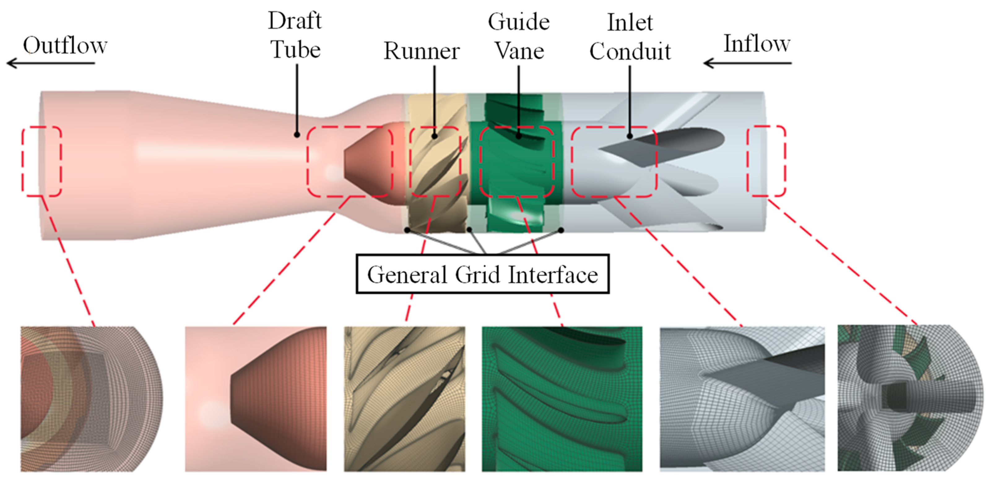
3.1.1. Fluid Domain

In this simulation experiment of this study, the fluid domain model includes 4 parts: the inlet conduit part, guide vane, runner, and draft tube. The vortex rope flow is mainly studied in the draft tube. However, the other parts provide the correct flow condition for the vortical flow in the draft tube. The fluid domain is shown in Figure 2.

3.1.2. Turbulence Model

The commercial software ANSYS Fluent was used as the computational fluid dynamics (CFD) solver in this study. Moreover, the detached eddy simulation was used, which is a zonal hybrid model of the Reynolds-averaged turbulence solution and large eddy simulation (LES). The Reynolds-averaged part depends on the shear stress transport (SST) model [41]. When using SST-DES, if the eddy scale is larger than the grid scale, LES is activated to provide a better solution of flow details. Moreover, the SST model was used for turbulence to reduce the grid number and also provide a good solution for engineering cases.

3.1.3. CFD Setup

The inflow of the inlet conduit was set as the velocity inlet boundary where the velocity is normal to the boundary (following the Z-axis in Figure 1). The outflow of the draft tube was set as the pressure outlet boundary with a relative static pressure value. All the walls were modeled as no-slip wall-type boundaries. Grid interfaces are provided between each of the two domains. The maximum iteration number for unsteady simulation was 45 for each time step, and the convergence criterion was set to 1 × 10⁻⁵ for the root-mean-square residual of continuity and momentum equations. The unsteady simulation should be executed in no less than 10 runner revolutions to obtain a correct result. The grid used in this CFD study is shown in

Table 2. Details of the CFD grid.

Domains	Element Number
Draft tube	5,056,300
Runner	546,250
Guide vane	636,025
Inlet conduit	284,307
Total	6,522,882

, which was tested in a previous study [12]. The CFD grid has approximately 6.5 million elements in total, with refinements mainly in the draft tube, which has approximately 5.1 million elements. Some enlarged views of the grid are shown in Figure 1.

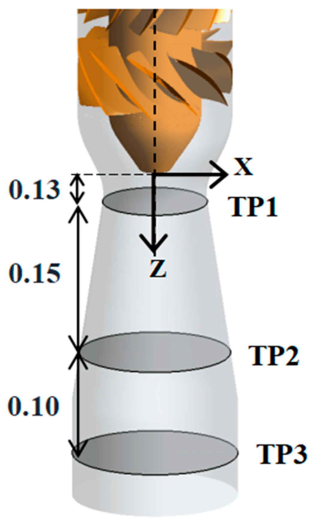
3.2. Monitoring Points for DMD Data

We set up monitoring points on the TP1, TP2, and TP3 sections to obtain the data required for the DMD method. Figure 3 shows the distribution of three sections, and the vortex rope extending from cone to cone receives detailed monitoring and analysis in these three sections. The monitoring point is a circle with the intersection point of the Z-axis and the plane as the origin and the intersection line between the plane and the wall as the boundary. The maximum distance between each monitoring point is defined as D_E. The calculation formula of D_E is

$$D_E=\frac{C_s{v}_{ref}}{2\pi f_{ref}}$$

(2)

where v_ref is the reference velocity, which is equal to the inlet axial velocity v_i, and f_ref is the reference frequency, which is approximately 15.33 Hz in this study. In order to optimize the distribution and resolution of monitoring points, the scaling factor, C_s, was initially set between 0.05 and 0.07. After calculation, the D_E value was within 0.88~1.23 mm, so the monitoring point numbers on TP1, TP2, and TP3 were 9040, 9521, and 10,012, respectively.

4. Verification and Validation

4.1. Experimental–Numerical Comparison

In order to ensure that the CFD simulation is in line with real-world scenarios, we compared the CFD results with the LDV velocity measurement experiment for a flow rate Q of 0.03 m³/s [39,40], and we converted the experimental results into dimensionless velocity to compare with the DES simulation results, verifying the reliability of the DES simulation results. Figure 4 shows the comparison curve and allowable error range of two experimental results, using data from ML1, ML2, and ML3 positions (see Figure 1) for comparison.

This paper presents the comparative data of LDV and IDDES (Improved Delayed Detached Eddy Simulation). From the comparison in Figure 4, it can be seen that the radial velocity comparison curve between the simulation results and the experimental results at ML1 basically coincides, while the tangential velocity comparison is very similar and within the allowable error range. The tangential velocity comparison at ML2 is very similar, while the radial velocity comparison curve is generally similar. Most of the curves are within the allowable error range, and the simulated data are generally accurate. The tangential velocity comparison curves at ML3 are generally coincident, while the radial velocity comparison curves are generally similar. Most of the curves are within the allowable error range, and the simulated data are also generally accurate. The reliability of CFD simulation can be verified by comparing the simulation results with experimental data. Therefore, the data obtained in this experiment can generally accurately predict the flow field structure in real-world scenarios.

4.2. Vortex Rope Flow Details

To quantify the pressure magnitude on each surface, dimensionless coefficients, C_p, are introduced. The formula for calculating these coefficients is as follows:

$$C_p=\frac{p-p_{ref}}{\frac{1}{2}\rho v_{ref}^2}$$

(3)

where $p_{ref}$ represents the boundary pressure at the inlet, $v_{ref}$ represents the inlet flow velocity $v_i$, $p$ represents the pressure magnitude at different locations in the flow field, and $\rho$ represents the density of water.

Figure 5 illustrates the flow field pattern in the draft tube when the inlet flow rate changes, providing an overview of the flow field morphology. Pressure cloud and flow vector maps were plotted in the TP1, TP2, and TP3 planes for the purpose of comparing and analyzing the flow state in these three planes.

At an inlet flow rate of v_i = 0.85 m/s, a cavity is formed in the vortex zone of the draft tube. In the TP1, TP2, and TP3 cross-sections, the pressure decreases from the edge to the center. The fluids in all cross-sections rotate in the same direction around the pressure minimum, and the rotation speed decreases with decreasing pressure. The TP1 cross-section exhibits a larger pressure change amplitude compared with the TP2 and TP3 cross-sections, indicating a clear low-pressure region. In all three cross-sections, there is a phenomenon of z-direction backflow in the low-pressure region, and the backflow rate increases with decreasing pressure. The backflow region in the TP1 cross-section is more centralized than in the TP2 and TP3 cross-sections.

At an inlet flow rate of v_i = 1.7 m/s, a spiral vortex band forms above the TP2 cross-section, while a vortex band below generates a cavity. In the TP1, TP2, and TP3 cross-sections, the pressure decreases from the edge to the center, and the fluid rotates in the same direction around the lowest pressure. As the pressure decreases, the fluid rotation speed decreases. The TP1 cross-section exhibits the largest pressure change amplitude and the most pronounced low-pressure region, while the TP3 cross-section shows the smallest pressure change amplitude and the least pronounced low-pressure region. Additionally, the low-pressure region in the TP2 and TP3 cross-sections experiences significant backflow, whereas the TP1 cross-section has only a small amount of backflow in the low-pressure region.

At an inlet flow rate of v_i = 3.4 m/s, a distinct spiral vortex band appears in the draft tube. In the TP2 and TP3 cross-sections, the pressure decreases from the edge to the center. In the TP1 cross-section, the pressure initially rises from the edge to the center and then decreases, resulting in a prominent low-pressure area at the center. Most of the fluid in the TP2 and TP3 cross-sections rotates around the lowest pressure, and the rotation speed is lowest in the low-pressure region. In the TP1 cross-section, the fluid rotates counterclockwise in the outside low-pressure area and clockwise in the inside low-pressure area. Overall, the TP1 section exhibits lower pressure compared with the TP2 and TP3 sections. The low-pressure regions in the TP2 and TP3 sections experience some backflow, while no backflow occurs in the TP1 section.

At the same time, the vorticity was calculated, and the vorticity cloud picture is shown in Figure 6, so that the rotation intensity under different conditions can be compared more intuitively. The calculation formula for vorticity is as follows:

$$Q^{*}=-\frac{1}{2}[{\left(\frac{\partial u}{\partial x}\right)}^2+{\left(\frac{\partial v}{\partial y}\right)}^2{+\left(\frac{\partial w}{\partial z}\right)}^2+2\frac{\partial u}{\partial y}\frac{\partial v}{\partial x}+2\frac{\partial u}{\partial z}\frac{\partial w}{\partial x}+2\frac{\partial v}{\partial z}\frac{\partial w}{\partial y}]$$

(4)

In the case of three different inlet velocities, obvious forward and reverse vortices appeared in the middle part of the TP1 plane at the same time. While only positive vortices appeared in the TP2 and TP3 planes, only a small number of insignificant reversals appeared in the edge part. This is consistent with the results of stress analysis. At an inlet flow rate of v_i = 3.4 m/s, on the TP3 plane, in addition to most of the positive vortices, a small number of reverse vortices appear.

Finally, we calculated the swirl parameter, S, of the model [42].

Table 3. The calculation results of S under different working conditions.

${\mathit{v}}_{\mathit{i}}$/(m/s)	0.85	1.7	3.4
TP1	0.923	0.779	4.395
TP2	0.868	0.587	2.042
TP3	0.352	0.612	1.555

shows the calculation results of S under different working conditions. The calculation formula of the swirl parameter is as follows:

$$S=\frac{{\int }_0^{\infty }\left(\rho uw+\rho \overline{u’w’}\right)r^{2}dr}{R{\int }_0^R\left[\rho u^2+\rho \overline{{u’}^2}+\left(p-p_{\infty }\right)\right]rdr}$$

(5)

where u represents the time-averaged axial velocity, w represents the time-averaged tangential velocity, p represents the pressure, r represents the radial coordinates, and u′ and w′ are turbulent fluctuations. However, in real working conditions it is very complicated to measure the spatial distribution of momentum components and pressure, and the turbulent shear stress and axial pressure gradient are generally ignored; therefore, Formula (4) can be simplified to the following formula:

$$S=\frac{{\int }_0^{\infty }\rho uw{r}^{2}dr}{R{\int }_0^R\rho u^{2}rdr}$$

(6)

5. Dynamic Mode Decomposition (DMD)

5.1. Method of DMD

The dynamic mode decomposition (DMD) method is based on matrix transformation, which can extract flow field structures with specific frequencies from flow field quantities. When using the DMD method, the snapshot sequence, X, of the real flow field information should be obtained based on the flow field snapshot sequence. On this basis, the following two data matrices are formed from the snapshot sequence:

$$X_1=\left[\begin{array}{cccc}|& |& & |\\ x\left(t_1\right)& x\left(t_2\right)& \dots & x\left(t_{n-1}\right)\\ |& |& & |\end{array}\right]$$

(7)

$$X_2=\left[\begin{array}{cccc}|& |& & |\\ x\left(t_2\right)& x\left(t_3\right)& \dots & x\left(t_n\right)\\ |& |& & |\end{array}\right]$$

(8)

Assuming that the snapshot is a discrete linear system, the following equations can be used:

$$x_n=A\ast x_{n-1}$$

(9)

$$X_2=A\ast X_1$$

(10)

A contains the specific information of the entire flow field snapshot. Based on singular value decomposition, A can be calculated using the following equations:

$$X_1=U\sum V^T$$

(11)

$$A=U^T{X}_{2}V{\sum }^{-1}$$

(12)

By applying the eigenvalue decomposition of A, the eigenvalue λ_j and eigenvector ω_j can be obtained. The mode of A can be evaluated using the following equation:

$$\varnothing =U\ast \omega$$

(13)

To determine the main mode of the flow field, the mode amplitude, α, is defined as the mode’s contribution to the initial snapshot by using the following equation:

$$\alpha =W^{-1}U{x}_1$$

(14)

By ordering the modes on the basis of the α values, the real-world scenario of the flow field can be predicted.

5.2. Results of Dynamic Mode Decomposition

In this experiment, the DMD (dynamic mode decomposition) analysis method was performed on the computational results of the model for three monitoring surfaces: TP1, TP2, and TP3. The analysis was conducted under three working conditions with inlet flow rates of v_i = 0.85, 1.7, and 3.4 m/s. The modes of each order obtained from the DMD analysis were sorted based on their energy magnitude. The energy of each mode was compared with the overall energy, and the proportion of the energy contributed by the first i order modes to the overall energy was calculated. Modes with a high energy share were selected to display their mode plots. In the DMD analysis results, conjugate modes refer to pairs of modes that have different energy contributions but share the same frequency and flow field pressure distribution. These modes are often observed in dynamic mode decomposition (DMD) analysis when analyzing complex flow fields.

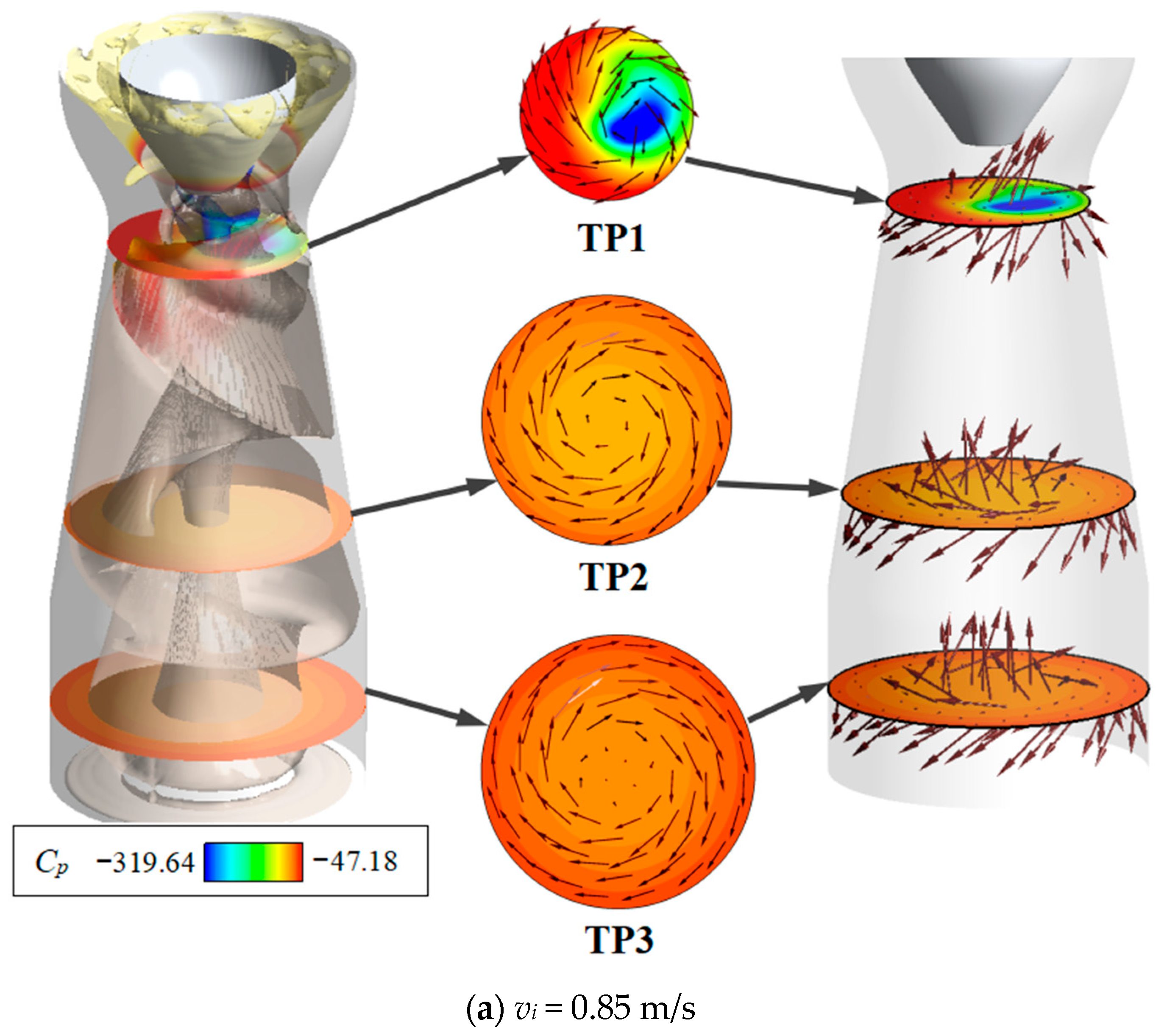
5.2.1. The Case of v_i = 0.85 m/s

Figure 7 illustrates the mode diagrams of the TP1 cross-section at the 0.85 m/s inlet flow rate condition for the first five modes. Among these modes, the first and second and the fourth and fifth modes are conjugate modes, representing the same frequency and flow field pressure distribution. The first two modes are low-frequency modes characterized by low-pressure regions distributed at the edge and high-pressure regions concentrated in the interior of the cross-section. The third mode is affected by the noise. As the ratio of the mode frequency to the reference frequency increases, the overall pressure of the mode increases, and the high- and low-pressure regions become concentrated inside the cross-section, with the medium-pressure region distributed at the cross-section’s edge.

Figure 8 shows the mode diagrams of the TP2 cross-section at the 0.85 m/s inlet flow rate condition for the first five modes. Among these modes, the second and third and the fourth and fifth modes are conjugate modes. As the ratio of the mode frequency to the reference frequency increases, the low-pressure region of the cross-section gradually shifts from the interior to the exterior, and the second and third modes exhibit higher overall pressure compared with the remaining modes.

Figure 9 displays the mode diagrams of the TP3 cross-section at the 0.85 m/s inlet flow rate condition for the first five modes. Among these modes, the fifth and sixth modes are conjugate modes. The second, third, and fourth modes are affected by the noise. The second-order modes have smaller overall pressure, with the high-pressure region concentrated in the interior of the cross-section and the pressure gradually decreasing from the center to the edge. The remaining modes exhibit larger overall pressures, with the low-pressure regions distributed in the interior of the cross-section. The overall pressure difference across the cross-section decreases as the ratio of the mode frequency to the reference frequency increases.

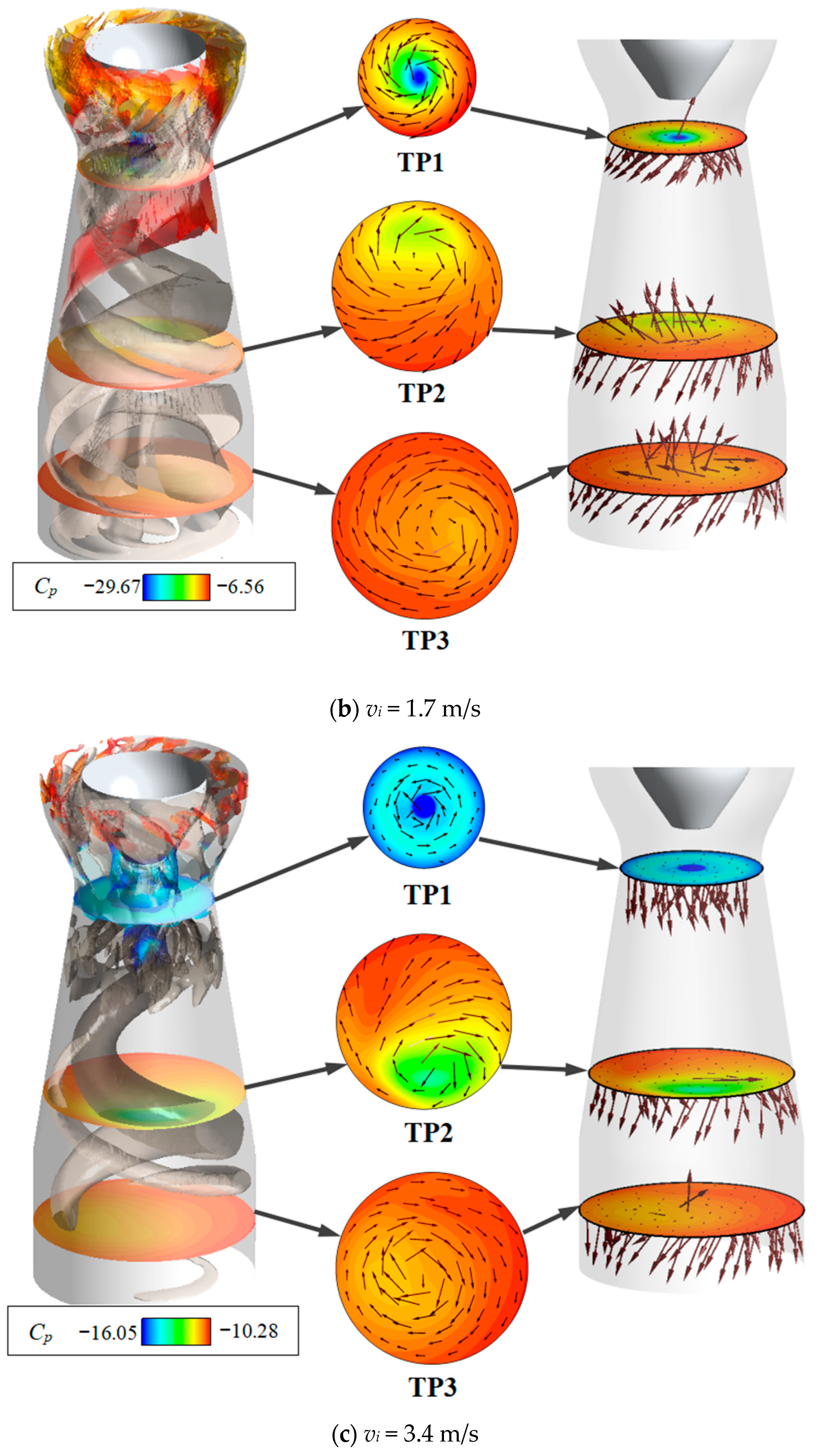
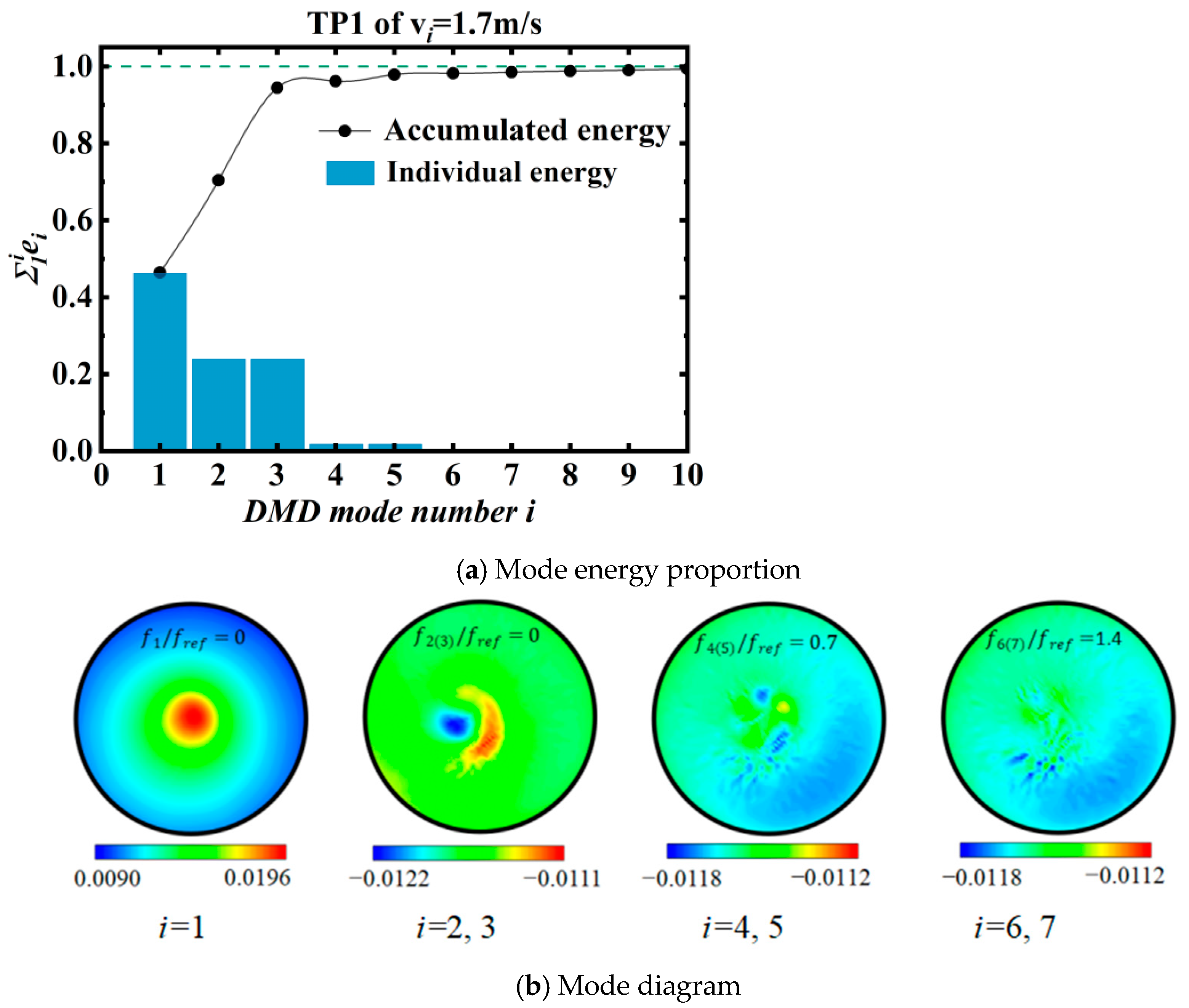
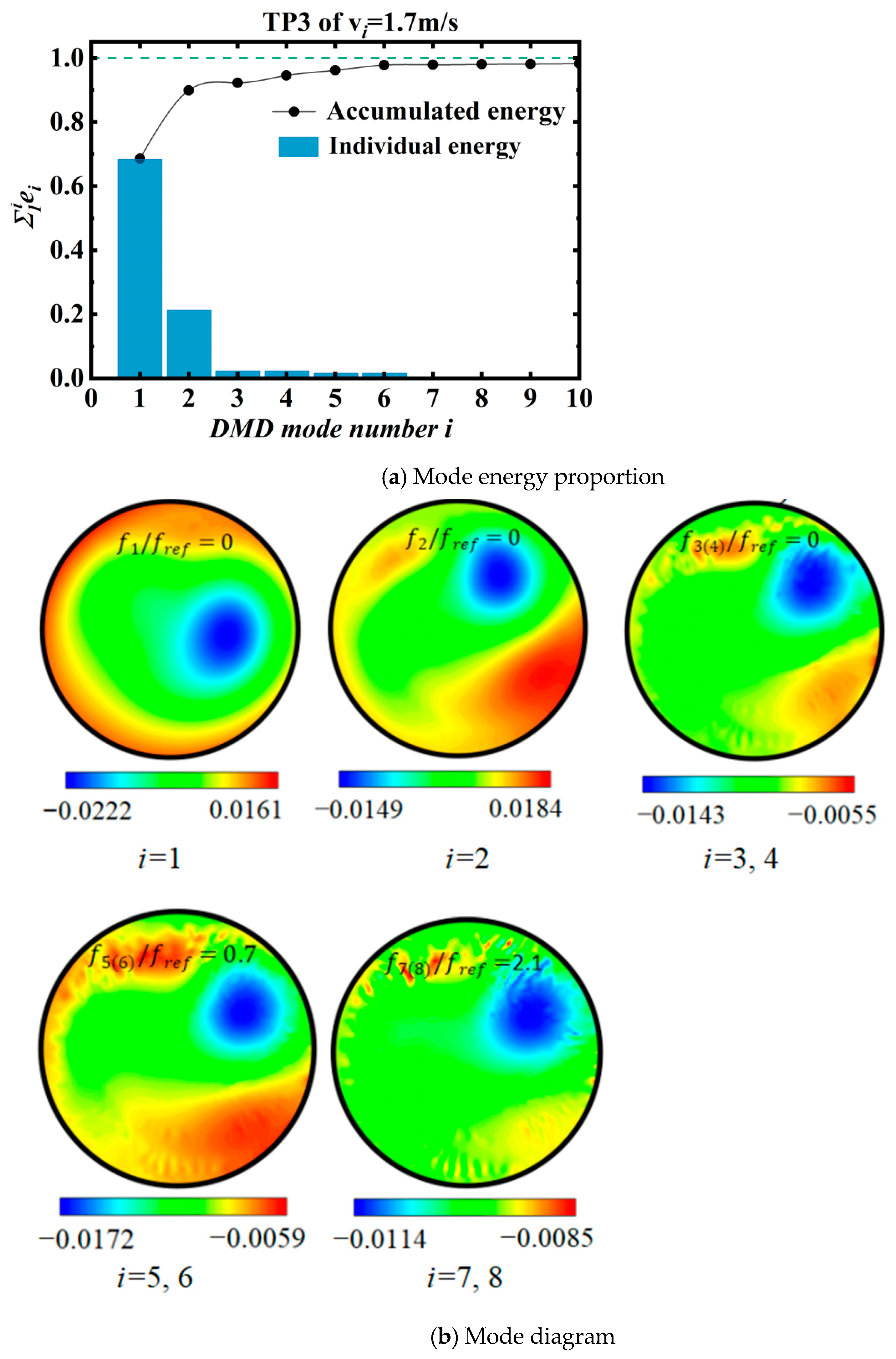
5.2.2. The Case of v_i = 1.7 m/s

Figure 10 shows the mode diagram of the TP1 cross-section under the 1.7 m/s inlet flow rate condition for the first seven modes. The second and third, fourth and fifth, and sixth and seventh modes are conjugate modes. In the low-frequency modes (with a ratio of mode frequency to reference frequency of 0), the high-pressure region is concentrated in the interior of the cross-section, while the low-pressure region shifts from the edge to the middle. As the ratio of the mode frequency to the reference frequency increases, the cross-section as a whole shows a large low-pressure distribution with a small pressure difference.

Figure 11 presents the mode diagram of the TP2 cross-section under the 1.7 m/s inlet flow rate condition for the first six modes. Among them, the fourth and fifth modes are conjugate modes. The second, third, and sixth modes are affected by the noise. In the low-frequency modes, the high-pressure region shifts from the interior to the edge of the cross-section, and the medium-pressure region expands, while the high-pressure and low-pressure regions shrink. As the ratio of the mode frequency to the reference frequency increases, the cross-section as a whole shows a medium-pressure distribution, with high-pressure and low-pressure areas appearing only at the edges.

Figure 12 shows the mode diagram of the TP3 cross-section under the 1.7 m/s inlet flow rate condition for the first seven modes. The third and fourth, fifth and sixth, and seventh and eighth modes are conjugate modes. The second mode is affected by the noise. The low-pressure region of the cross-section is concentrated in the interior, while the high-pressure region is distributed at the edge in different modes. As the ratio of the mode frequency to the reference frequency increases, the maximum pressure of the cross-section decreases.

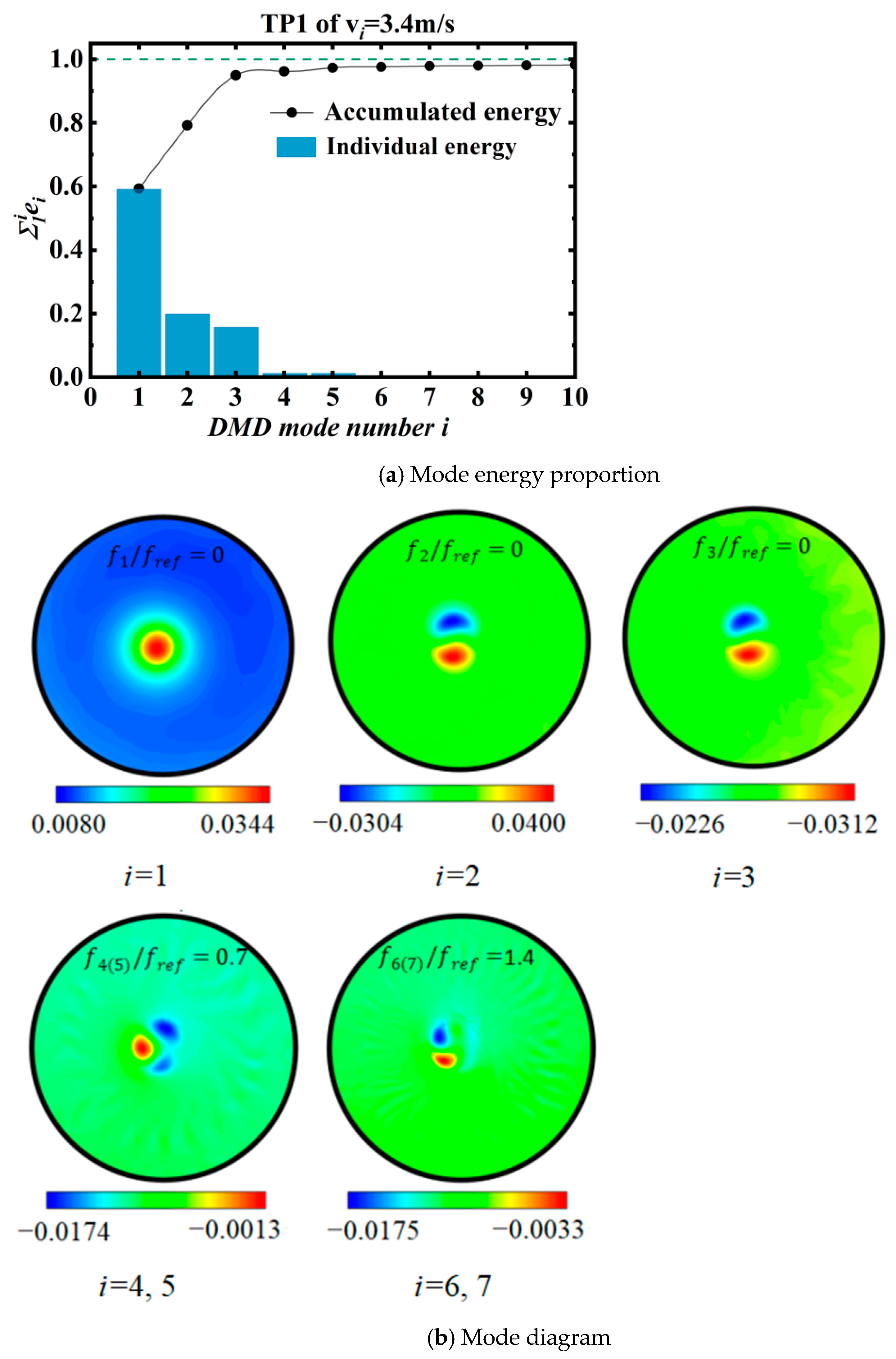
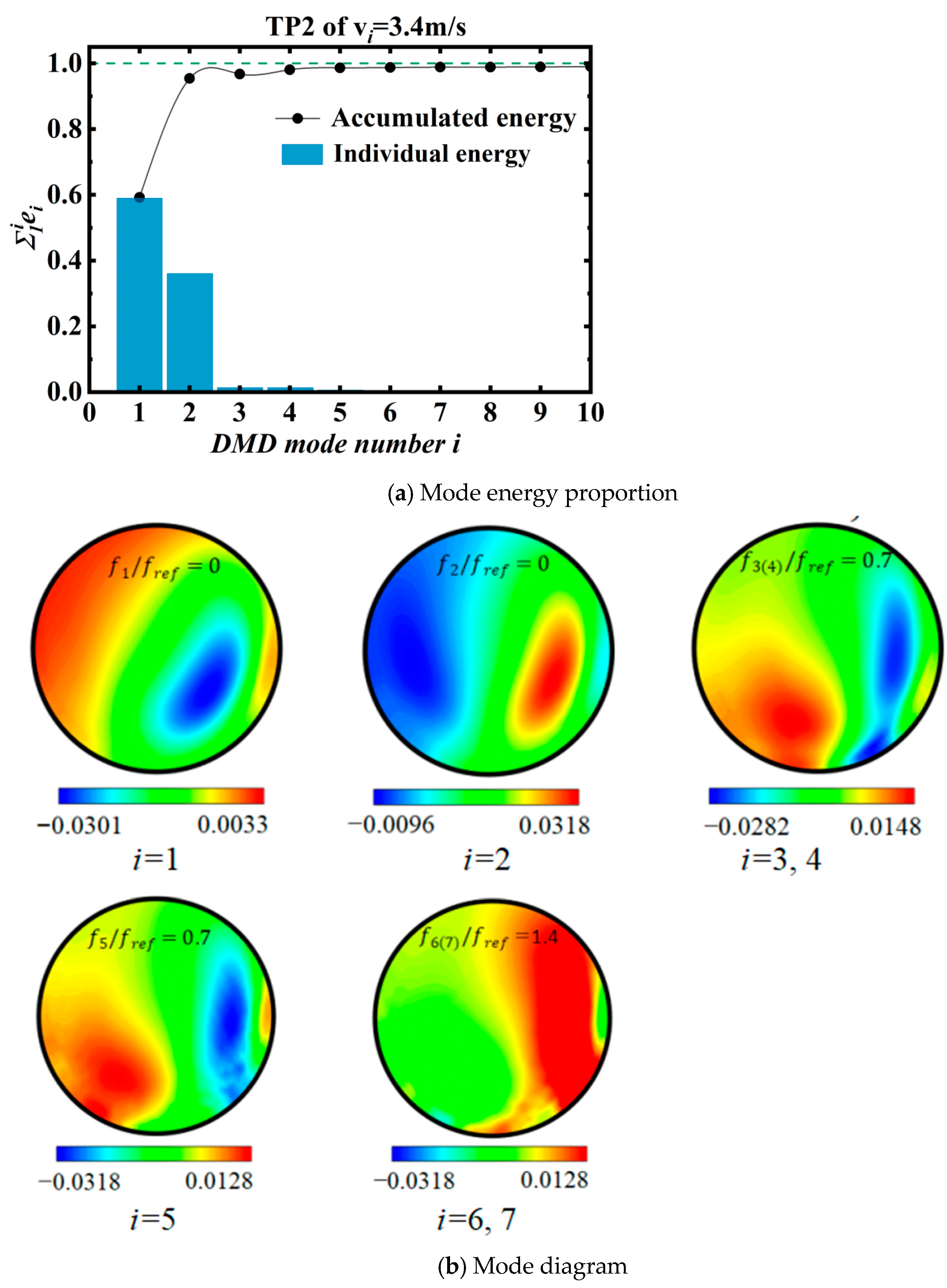
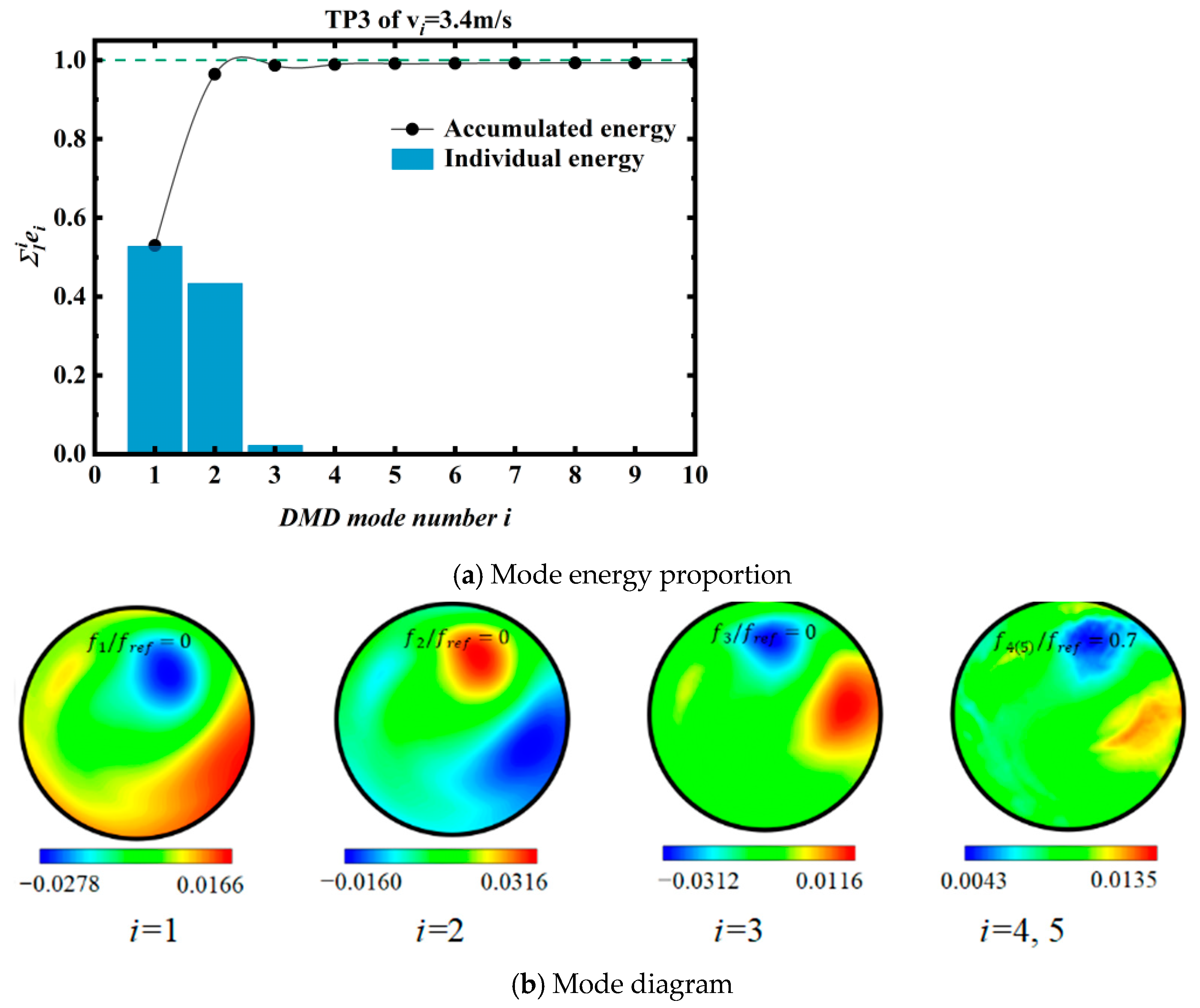
5.2.3. The Case of v_i = 3.4 m/s

Figure 13 shows the mode diagram of the TP1 cross-section under the 3.4 m/s inlet flow rate condition for the first seven modes. The fourth and fifth and the sixth and seventh modes are conjugate modes. The second and third modes are affected by the noise. In the 1st mode, the high-pressure region of the cross-section is concentrated in the center, while the low-pressure region has a larger distribution range at the edge. In the remaining modes, the high-pressure region is concentrated in the interior of the cross-section and the medium-pressure region has a larger range. In the higher-frequency modes, the change in cross-section pressure is small as the ratio of the mode frequency to the reference frequency increases.

Figure 14 illustrates the mode diagram of the TP2 cross-section under the 3.4 m/s condition for the first seven modes. The third and fourth and the sixth and seventh modes are conjugate modes. The second and fifth modes are affected by the noise. In the low-frequency modes, except for the second mode, the low-pressure region is concentrated inside the cross-section. In the high-frequency modes, the low-pressure region becomes less pronounced and the distribution of the medium-pressure and high-pressure regions becomes more evident. As the ratio of the mode frequency to the reference frequency increases, the high-pressure region gradually expands.

Figure 15 demonstrates the mode diagram of the TP3 cross-section under the 3.4 m/s condition for the first five modes. The fourth and fifth modes are conjugate modes and the second and third modes are affected by the noise. Except for the second mode, the low-pressure region of the cross-section is centrally distributed in the interior. With an increase in the ratio of the mode frequency to the reference frequency, the distribution range of the high-pressure region gradually decreases and the overall pressure of the cross-section increases.

6. Conclusions

Through research based on flow simulation and mode decomposition, the most significant innovation of this study is that it reflects the changes in corresponding flow characteristics with the flow rate or flow velocity conditions through the strength of different modes. In the past, when looking at the impact of flow or velocity on flow, it was not possible to clearly identify which characteristics were changing, but this study provides intuitive results. The following conclusions were drawn:

(1)

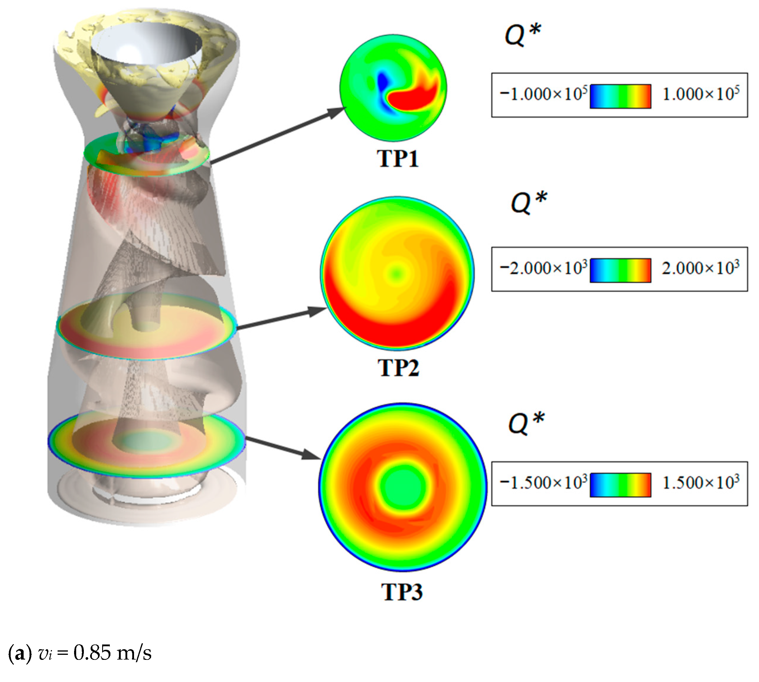
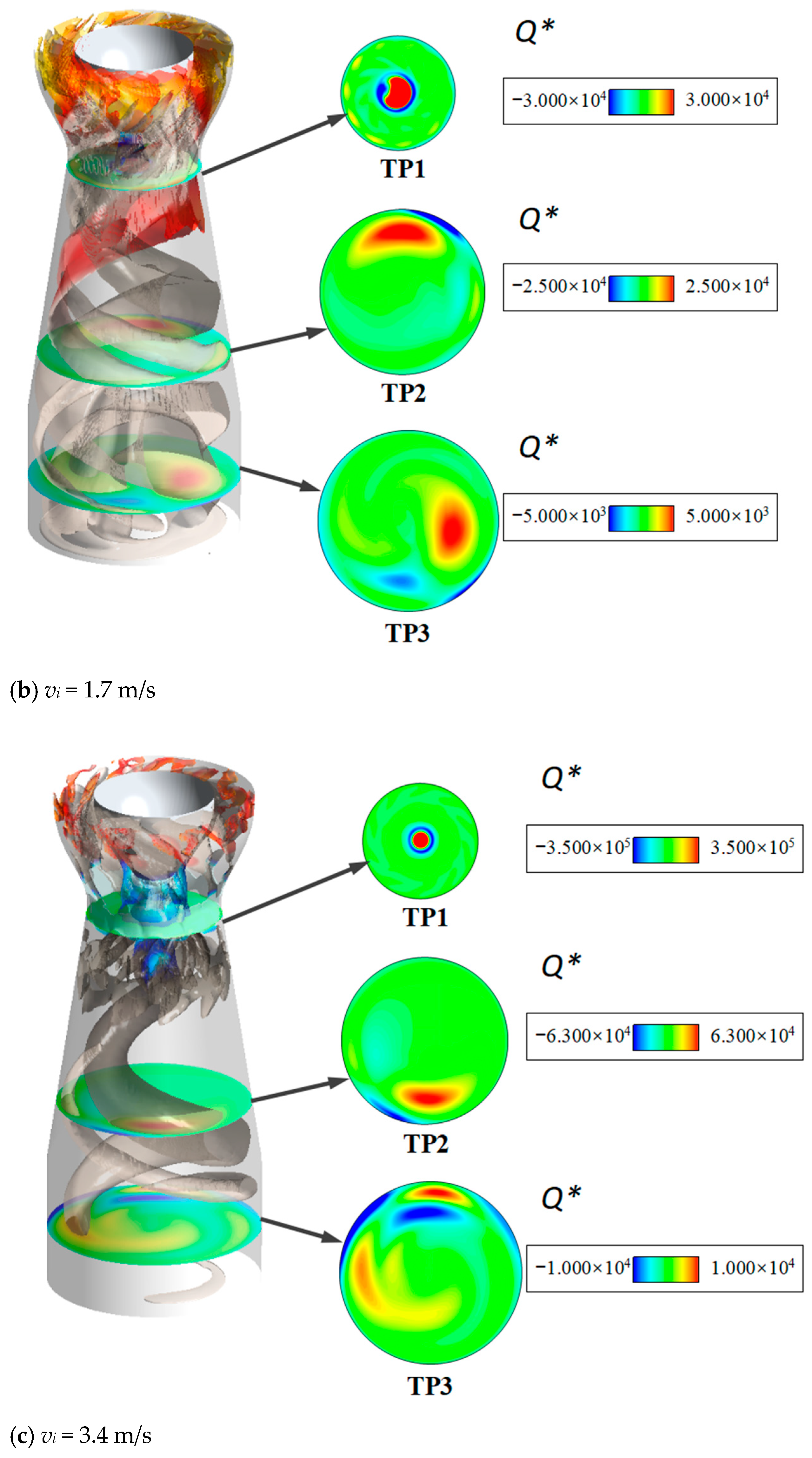
The influence of flow rate or velocity on flow pattern is well known, but when there are rotating components its impact is reflected in the uncontrolled vortex flow downstream, and the specific magnitude of its impact still requires special qualitative or quantitative analysis. When the inlet flow velocity is v_i = 0.85 m/s, a core forms in the vortex zone of the draft tube and the fluid rotates in the same direction around the lowest pressure point of the cross-section. The backflow phenomenon occurs in the low-pressure region. When the inlet flow velocity is v_i = 1.7 m/s, a spiral vortex rope forms above the draft tube and a core forms below. The fluid still rotates in the same direction around the lowest pressure point of the section, and the backflow of the TP1 section is reduced. When the inlet flow velocity is v_i = 3.4 m/s, there is a significant spiral vortex rope in the draft tube and the fluid at the TP1 section rotates in two directions, resulting in the disappearance of the backflow phenomenon in the flow field.

(2)

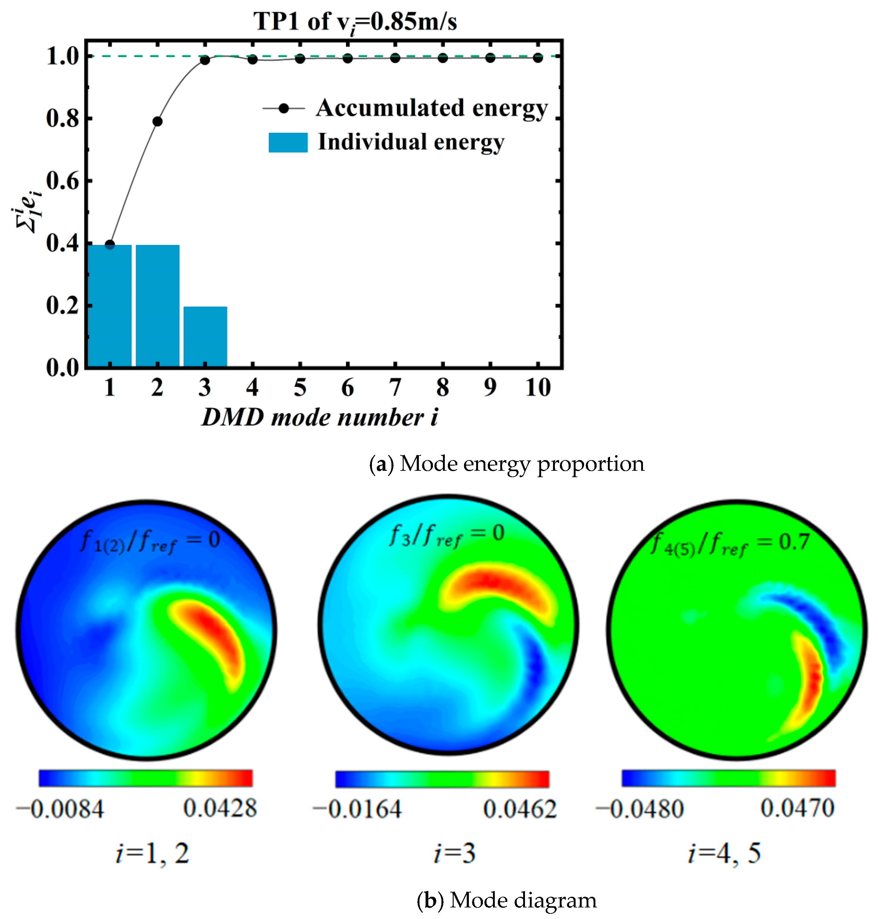
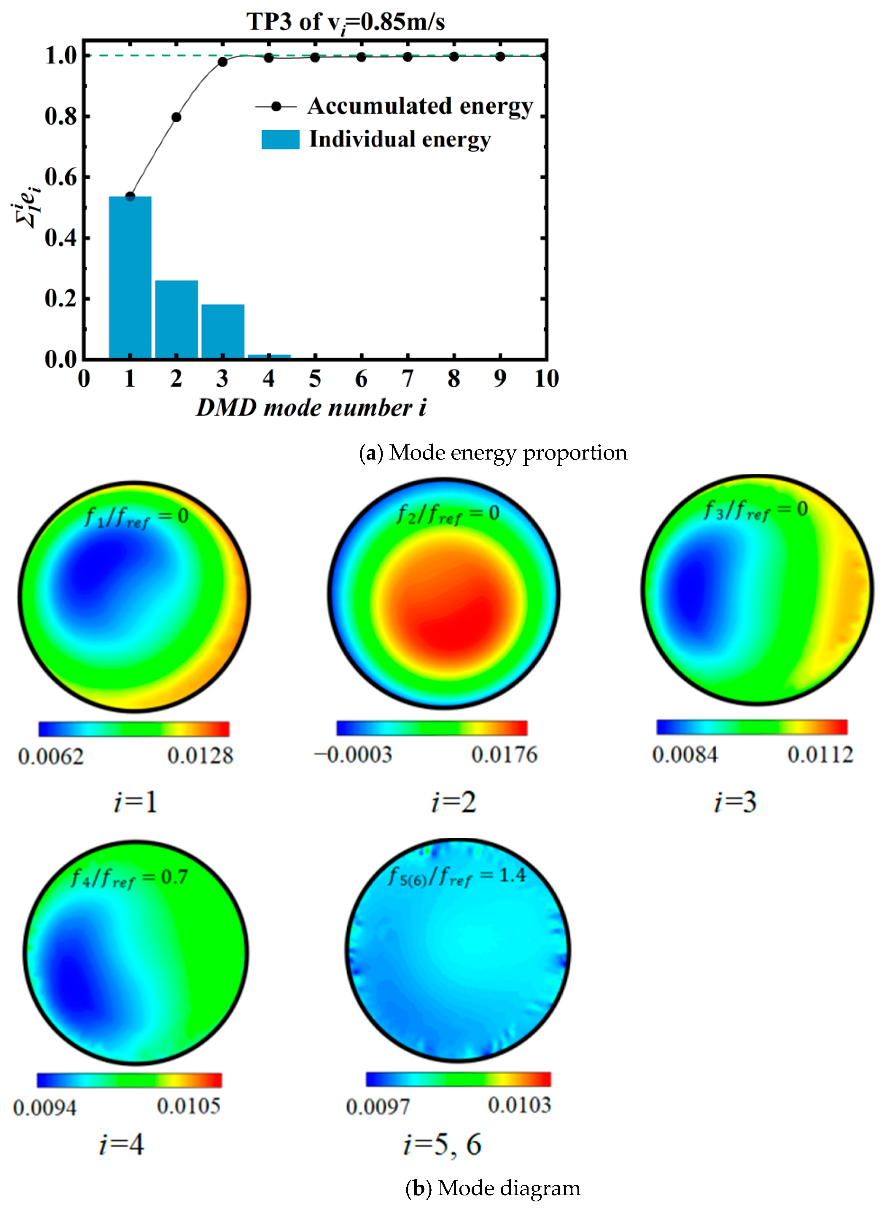
Fourier-transform analysis was performed on the high-energy modes decomposed from the DMD analysis, and the relative frequencies of the modes against the reference frequency were obtained as 0 (averaged), 0.7, and 1.4, respectively. The eigenvalues corresponding to the first mode are real numbers with a relative frequency of 0, indicating that the flow corresponding to this mode is time-averaged, representing the average flow mode of the velocity field. Due to the fact that the vortex rope is runner-driven and always undergoes periodic changes, its average feature is an important feature that is proved by this decomposition of a low-frequency conjugate mode with a relative frequency of 0.7, which is the low-frequency oscillation of the flow field superimposed on the basic structure. This component below the runner frequency is a representative pulsation frequency component of the vortex rope, and it is also the main motion law of the vortex rope found in the past. The feature extraction via mode decomposition was successful and correct. A high-frequency conjugate mode with a relative frequency of 1.4 refers to the high-frequency oscillation of the flow field superimposed on the basic structure. This is related to the turbulent flow changes in the rotation process of the vortex rope itself.

(3)

As the inlet velocity increases, the order of high-energy modes increases and the high-frequency oscillations superimposed on the basic structure by the unsteady flow in the flow field increase. At v_i = 0.85 m/s, the backflow phenomenon at the TP1 section is influenced by low-frequency modes, while the backflow phenomenon at the TP2 and TP3 sections is influenced by the first-order mode time average flow. When v_i = 1.7 m/s, the TP1 section in the spiral vortex zone region is affected by the second- and third-order modes, the backflow phenomenon of the TP2 section is influenced by the first-order modal time average flow, and the TP3 cross-section in the cavity region is affected by low-frequency and first-order modes. When v_i = 3.4 m/s, the clockwise rotation of the vortex band is influenced by the combination of high-frequency and low-frequency modes. The TP1 section has the joint influence of high-frequency and low-frequency modes. The backflow phenomenon at the TP2 and TP3 cross-sections is influenced by low-frequency and first-order modes. Overall, when the flow rate or flow velocity is too high or too low, the vortex rope of the draft tube experiences a weakening or strengthening of the rotational component, with specific modes other than the mean field dominating and the number of high-energy modes decreasing. When the flow rate conforms to the control of the runner, the modes are relatively balanced, which is reflected in a higher number of high-energy modes.

References

1. Hunt, J.D.; Byers, E.; Wada, Y.; Parkinson, S.; Gernaat, D.E.H.J.; Langan, S.; van Vuuren, D.P.; Riahi, K. Global resource potential of seasonal pumped hydropower storage for energy and water storage. Nat. Commun. 2020, 11, 947. [Google Scholar] [CrossRef] [PubMed]
2. Lund, P.D. Clean energy systems as mainstream energy options: Clean energy systems. Int. J. Energy Res. 2016, 40, 4–12. [Google Scholar] [CrossRef]
3. Xu, B.; Chen, D.; Venkateshkumar, M.; Xiao, Y.; Yue, Y.; Xing, Y.; Li, P. Modeling a pumped storage hydropower integrated to a hybrid power system with solar-wind power and its stability analysis. Appl. Energy 2019, 248, 446–462. [Google Scholar] [CrossRef]
4. Li, C.; Mao, Y.; Yang, J.; Wang, Z.; Xu, Y. A nonlinear generalized predictive control for pumped storage unit. Renew. Energy 2017, 114, 945–959. [Google Scholar] [CrossRef]
5. Tao, R.; Lu, J.; Jin, F.; Hu, Z.; Zhu, D.; Luo, Y. Evaluation of the rotor eccentricity added radial force of oscillating water column. Ocean Eng. 2023, 276, 114222. [Google Scholar] [CrossRef]
6. Trivedi, C.; Cervantes, M.J. Fluid-structure interactions in Francis turbines: A perspective review. Renew. Sustain. Energy Rev. 2017, 68, 87–101. [Google Scholar] [CrossRef]
7. Tokyay, T.E.; Constantinescu, S.G. Validation of a Large-Eddy Simulation Model to Simulate Flow in Pump Intakes of Realistic Geometry. J. Hydraul. Eng. 2006, 132, 1303–1315. [Google Scholar] [CrossRef]
8. Stefan, D.; Hudec, M.; Uruba, V.; Procházka, P.; Urban, O.; Rudolf, P. Experimental investigation of swirl number influence on spiral vortex structure dynamics. In Proceedings of the 30th IAHR Symposium on Hydraulic Machinery and Systems (IAHR 2020), Lausanne, Switzerland, 21–26 March 2021; Volume 774. [Google Scholar]
9. Wen, F.F.; Cheng, Y.G.; You, J.F.; Li, T.C.; Hu, H.P.; Gao, L.J.; Yang, F. Cavitation pressure fluctuation characteristics of a prototype pump-turbine analysed by using CFD. IOP Conf. Ser. Earth Environ. Sci. 2019, 240, 72035. [Google Scholar] [CrossRef]
10. Zhang, N.; Liu, X.; Gao, B.; Xia, B. DDES analysis of the unsteady wake flow and its evolution of a centrifugal pump. Renew. Energy 2019, 141, 570–582. [Google Scholar] [CrossRef]
11. Goyal, R.; Cervantes, M.J.; Gandhi, B.K. Vortex Rope Formation in a High Head Model Francis Turbine. J. Fluids Eng.-Trans. ASME 2017, 139, 041102. [Google Scholar] [CrossRef]
12. Jin, F.; Li, P.; Tao, R.; Xiao, R.; Zhu, D. Study of vortex rope for the flow field pulsation law. Ocean Eng. 2023, 273, 114026. [Google Scholar] [CrossRef]
13. Yu, A.; Zou, Z.; Zhou, D.; Zheng, Y.; Luo, X. Investigation of the correlation mechanism between cavitation rope behavior and pressure fluctuations in a hydraulic turbine. Renew. Energy 2020, 147, 1199–1208. [Google Scholar] [CrossRef]
14. Michihiro, N.; Liu, S. An Outlook on the Draft-Tube-Surge Study. Int. J. Fluid Mach. Syst. 2013, 6, 33–48. [Google Scholar]
15. Wang, L.; Cui, J.; Shu, L.; Jiang, D.; Xiang, C.; Li, L.; Zhou, P. Research on the Vortex Rope Control Techniques in Draft Tube of Francis Turbines. Energies 2022, 15, 9280. [Google Scholar] [CrossRef]
16. Yang, J.; Zhou, L.J.; Wang, Z.W. The numerical research of runner cavitation effects on spiral vortex rope in draft tube of Francis turbine. In Proceedings of the 9th International Symposium on Cavitation (CAV2015), Lausanne, Switzerland, 6–10 December 2015; Volume 656. [Google Scholar]
17. Ni, Y.; Zhu, R.; Zhang, X.; Pan, Z. Numerical investigation on radial impeller induced vortex rope in draft tube under partial load conditions. J. Mech. Sci. Technol. 2018, 32, 157–165. [Google Scholar] [CrossRef]
18. Skripkin, S.; Tsoy, M.; Kuibin, P.; Shtork, S. Vortex rope patterns at different load of hydro turbine model. MATEC Web Conf. 2017, 115, 06004. [Google Scholar] [CrossRef]
19. Sotoudeh, N.; Maddahian, R.; Cervantes, M.J. Investigation of Rotating Vortex Rope formation during load variation in a Francis turbine draft tube. Renew. Energy 2020, 151, 238–254. [Google Scholar] [CrossRef]
20. Luo, X.; Yu, A.; Ji, B.; Wu, Y.; Tsujimoto, Y. Unsteady vortical flow simulation in a Francis turbine with special emphasis on vortex rope behavior and pressure fluctuation alleviation. Proc. Inst. Mech. Eng. Part A-J. Power Energy 2017, 231, 215–226. [Google Scholar] [CrossRef]
21. Liu, C.; Wang, Y.; Yang, Y.; Duan, Z. New omega vortex identification method. Sci. China Phys. Mech. Astron. 2016, 59, 1–9. [Google Scholar] [CrossRef]
22. Ji, L.; Xu, L.; Peng, Y.; Zhao, X.; Li, Z.; Tang, W.; Liu, D.; Liu, X. Experimental and Numerical Simulation Study on the Flow Characteristics of the Draft Tube in Francis Turbine. Machines 2022, 10, 230. [Google Scholar] [CrossRef]
23. Kim, S.; Suh, J.; Choi, Y.; Park, J.; Park, N.; Kim, J. Inter-Blade Vortex and Vortex Rope Characteristics of a Pump-Turbine in Turbine Mode under Low Flow Rate Conditions. Water 2019, 11, 2554. [Google Scholar] [CrossRef]
24. Yu, Z.; Yan, Y.; Wang, W.; Liu, X. Entropy production analysis for vortex rope of a Francis turbine using hybrid RANS/LES method. Int. Commun. Heat Mass Transf. 2021, 127, 105494. [Google Scholar] [CrossRef]
25. Li, P.; Xiao, R.; Tao, R. Study of vortex rope based on flow energy dissipation and vortex identification. Renew. Energy 2022, 198, 1065–1081. [Google Scholar] [CrossRef]
26. Jafarzadeh Juposhti, H.; Maddahian, R.; Cervantes, M.J. Optimization of axial water injection to mitigate the Rotating Vortex Rope in a Francis turbine. Renew. Energy 2021, 175, 214–231. [Google Scholar] [CrossRef]
27. Zhou, X.; Wu, H.; Shi, C. Numerical and experimental investigation of the effect of baffles on flow instabilities in a Francis turbine draft tube under partial load conditions. Adv. Mech. Eng. 2019, 11, 2072051534. [Google Scholar] [CrossRef]
28. Sun, L.; Li, Y.; Guo, P.; Xu, Z. Numerical investigation of air admission influence on the precessing vortex rope in a Francis turbine. Eng. Appl. Comput. Fluid Mech. 2023, 17, 2164619. [Google Scholar] [CrossRef]
29. Nicolet, C.; Zobeiri, A.; Maruzewski, P.; Avellan, F. Experimental investigations on upper part load vortex rope pressure fluctuations in Francis turbine draft tube. Int. J. Fluid Mach. Syst. 2011, 4, 179–190. [Google Scholar] [CrossRef]
30. Begiashvili, B.; Groun, N.; Garicano-Mena, J.; Le Clainche, S.; Valero, E. Data-driven mode decomposition methods as feature detection techniques for flow problems: A critical assessment. Phys. Fluids 2023, 35, 41301. [Google Scholar] [CrossRef]
31. Liu, M.; Tan, L.; Cao, S. Dynamic mode decomposition of cavitating flow around ALE 15 hydrofoil. Renew. Energy 2019, 139, 214–227. [Google Scholar] [CrossRef]
32. Vanierschot, M.; Ogus, G. Experimental investigation of the precessing vortex core in annular swirling jet flows in the transitional regime. Exp. Therm. Fluid Sci. 2019, 106, 148–158. [Google Scholar] [CrossRef]
33. Litvinov, I.; Sharaborin, D.; Gorelikov, E.; Dulin, V.; Shtork, S.; Alekseenko, S.; Oberleithner, K. Modal Decomposition of the Precessing Vortex Core in a Hydro Turbine Model. Appl. Sci. 2022, 12, 5127. [Google Scholar] [CrossRef]
34. Schmid, P.J. Dynamic mode decomposition of numerical and experimental data. J. Fluid Mech. 2010, 656, 5–28. [Google Scholar] [CrossRef]
35. Schmid, P.J.; Li, L.; Juniper, M.P.; Pust, O. Applications of the dynamic mode decomposition. Theor. Comput. Fluid Dyn. 2011, 25, 249–259. [Google Scholar] [CrossRef]
36. Li, Y.; He, C.; Li, J. Study on Flow Characteristics in Volute of Centrifugal Pump Based on Dynamic Mode Decomposition. Math. Probl. Eng. 2019, 2019, 2567659. [Google Scholar] [CrossRef]
37. Liu, M.; Tan, L.; Cao, S. Dynamic mode decomposition of gas-liquid flow in a rotodynamic multiphase pump. Renew. Energy 2019, 139, 1159–1175. [Google Scholar] [CrossRef]
38. Petit, O.; Bosioc, A.I.; Nilsson, H.; Muntean, S.; Susan-Resiga, R.F. Unsteady Simulations of the Flow in a Swirl Generator, Using OpenFOAM. International Int. J. Fluid Mach. Syst. 2011, 4, 199–208. [Google Scholar] [CrossRef]
39. Susan-Resiga, R.; Muntean, S.; Bosioc, A.; Stuparu, A.; Milos, T.; Baya, A.; Bernad, S.; Anton, L.E. Swirling flow apparatus and test rig for flow control in hydraulic turbines discharge cone. In Proceedings of the 2nd IAHR International Meeting Workgroup on Cavitation and Dynamic Problems in Hydraulic Machinery and Systems, Timisoara, Romania, 24–26 October 2007. [Google Scholar]
40. Javadi, A.; Bosioc, A.; Nilsson, H.; Muntean, S.; Susan-Resiga, R. Experimental and Numerical Investigation of the Precessing Helical Vortex in a Conical Diffuser, With Rotor—Stator Interaction. J. Fluids Eng.-Trans. ASME 2016, 138, 081106. [Google Scholar] [CrossRef]
41. Menter, F.R.; Kuntz, M.; Langtry, R. Ten Years of Industrial Experience with the SST Turbulence Model. Turbul. Heat Mass Transf. 2003, 4, 625–632. [Google Scholar]
42. Skripkin, S.; Tsoy, M.; Kuibin, P.; Shtork, S. Swirling flow in a hydraulic turbine discharge cone at different speeds and discharge conditions. Exp. Therm. Fluid Sci. 2019, 100, 349–359. [Google Scholar] [CrossRef]
Figure 1. Model of the turbine vortex rope generator.
Symmetry 16 00416 g001
Figure 2. The fluid domain model with grid details.
Symmetry 16 00416 g002
Figure 3. Distribution of monitoring points on three sections in the draft tube.
Symmetry 16 00416 g003
Figure 4. Experimental [38,39] numerical comparison and verification.
Symmetry 16 00416 g004
Figure 5. The flow field and flow regime at cross-sections of the draft tube.
Symmetry 16 00416 g005aSymmetry 16 00416 g005b
Figure 6. Numerical analysis of the simulated vorticity quantities.
Symmetry 16 00416 g006aSymmetry 16 00416 g006b
Figure 7. Mode energy proportion and mode diagram of TP1 cross-section of vi = 0.85 m/s.
Symmetry 16 00416 g007
Figure 8. Mode energy proportion and mode diagram of TP2 cross-section of vi = 0.85 m/s.
Symmetry 16 00416 g008aSymmetry 16 00416 g008b
Figure 9. Mode energy proportion and mode diagram of TP3 cross-section of vi = 0.85 m/s.
Symmetry 16 00416 g009
Figure 10. Mode energy proportion and mode diagram of TP1 cross-section of vi = 1.7 m/s.
Symmetry 16 00416 g010
Figure 11. Mode energy proportion and mode diagram of TP2 cross-section of vi = 1.7 m/s.
Symmetry 16 00416 g011
Figure 12. Mode energy proportion and mode diagram of TP3 cross-section of vi = 1.7 m/s.
Symmetry 16 00416 g012
Figure 13. Mode energy proportion and mode diagram of TP1 cross-section of vi = 3.4 m/s.
Symmetry 16 00416 g013
Figure 14. Mode energy proportion and mode diagram of TP2 cross-section of vi = 3.4 m/s.
Symmetry 16 00416 g014
Figure 15. Mode energy proportion and mode diagram of TP3 cross-section of vi = 3.4 m/s.
Symmetry 16 00416 g015