
An Exploration of Multitasking Scheduling Considering Interruptible Job Assignments, Machine Aging Effects, the Influence of Deteriorating Maintenance, and Symmetry

1
School of Statistics and Mathematics, Yunnan University of Finance and Economics, Kunming 650221, China
2
School of Mathematics and Statistics, Honghe University, Mengzi 661100, China
Symmetry 2024, 16(3), 380; https://doi.org/10.3390/sym16030380
Submission received: 27 February 2024
/
Revised: 13 March 2024
/
Accepted: 19 March 2024
/
Published: 21 March 2024
(This article belongs to the Special Issue Symmetry/Asymmetry in Operations Research)
Abstract
:The unique topic of allocating and scheduling tasks on a single machine in a multitasking environment is the main emphasis of this research, which also takes into account the effects of worsening maintenance and job-dependent aging effects. In this scenario, the performance and efficiency of the machine in handling different tasks should be symmetric, without significant bias due to the nature or size of the tasks. In a multitasking environment, waiting for jobs can disrupt the processing of the primary job being currently handled. As a result, the actual time required to complete a task becomes erratic and contingent upon the duration of the disruption. In addition to figuring out the best time for maintenance, where to put the due-window, and how big it should be in a multitasking environment, the primary objective is to minimize the costs associated with meeting due-window regulations. To tackle this problem, we propose two optimal algorithms. Additionally, we conduct numerical experiments to compare our approach with the classic due date assignment problem. Interestingly, we observe that in most cases, the average and minimum percentage costs tend to increase as the quantity of jobs increases. However, it is noteworthy that, when the number of jobs is relatively small, specifically when it does not exceed 20, there are instances where these costs decrease with an increase in the number of jobs.
1. Introduction
In the classical scheduling problem, a machine needs to complete a job before starting the next job. However, in some practical situations, the machine may be affected by other jobs or even be interrupted while processing the current job, so the time required for job completion will be changed. The mentioned phenomenon is referred to as multitasking, characterized by the concurrent execution of multiple tasks [1]. Multitasking usually occurs in various areas such as healthcare, administration, logistics, emergency care, etc. As an illustration, consider that in the healthcare field, hospital doctors spend 21% of their working time on multiple activities at the same time [2]; the physician might attend to a new patient or manage existing cases, all the while awaiting the outcomes of blood or diagnostic tests [3]. Attending physicians experienced interruptions approximately every 9 min on average, while residents encountered interruptions about every 14 min on average [4]. In the administration field, the administrator of a department at a university works with her team. Their work includes designing promotional programs for academic activities and writing annual reports. The administrator divides the work into different parts and arranges them for her colleagues. In addition to finishing her job, she has to invest time in reviewing the team’s advancements on all pending tasks and providing them with feedback [5]. Hall, Leung, and Li [5] first used the three-field notation of Graham et al. [6] to model multitasking scheduling. At present, some studies have found that multitasking can affect the efficiency of work. Salmon and Farm [7] estimate that, if the number of tasks increases from two to three, the loss of productivity will increase from 20% to 50%. Although most studies express the belief that multitasking can reduce efficiency, there are some exceptions. The numerical experiment of Hall, Leung, and Li [1] shows that, by selecting a smaller parameter value in a model, there is potential for a modest net benefit from multitasking.
Because metaheuristic algorithms can produce nearly optimal solutions within a reasonable time frame, the use of these algorithms in job scheduling has garnered significant attention in recent times. In the cloud and fog environment, Singh R M et al. [8] provide a thorough taxonomic overview and analysis of modern metaheuristic scheduling techniques utilizing extensive evaluation criteria. A novel metaheuristic approach for maximizing collaborative job scheduling in cloud data centers was put out by Alboaneen, Dabiah, et al. [9]. For additional findings on multitasking scheduling, readers may consult [10,11,12,13].
In the aforementioned example concerning multitasking administration, each significant task is accompanied by a designated due date, which serves as a performance metric for the administrator. To enhance realism, the utilization of a time interval, referred to as the due-window, presents a more accurate representation of a job’s deadline, rather than a singular time instant. This approach was initially explored by [14] in the field of scheduling with due-windows. Additional research conducted by Liman et al. [15] focused on single-machine scheduling with common due- windows. Huo, Yujia, et al. [16] investigated a multitasking scheduling problem with alternating periods and demonstrated its strong NP-hardness when jobs were released on different dates. Two polynomial methods were developed specially to solve the single-machine common due-window problem by Xu, Chen, et al. [17]. Traditional scheduling studies have typically assumed uninterrupted machine availability. However, it is important to acknowledge that machines may occasionally require maintenance, rendering them temporarily unavailable for job-processing. In response, Mosheiov and Sarig [18] extended the problem domain to incorporate maintenance activities as potential options for consideration. In certain actual production systems, the duration of machine maintenance may vary, depending on the machine’s running time. To enhance the realism of the problem, Yang [19] introduced a model considering learning, aging, and deteriorating maintenance. Building upon this, in a study on single-machine scheduling, Yin et al. [20] looked into generalized position-dependent degrading jobs, maintenance tasks that deteriorate over time, and assignment due dates.
Liu et al. [21], inspired by the research of Hall, Leung, and Li [5], conducted an investigation into the concurrent issues of multitasking scheduling and the widespread assignment of due dates on a solitary machine. Zhu, Zheng, and Chu [22] investigated rate-modifying activity multitasking scheduling challenges in humans.
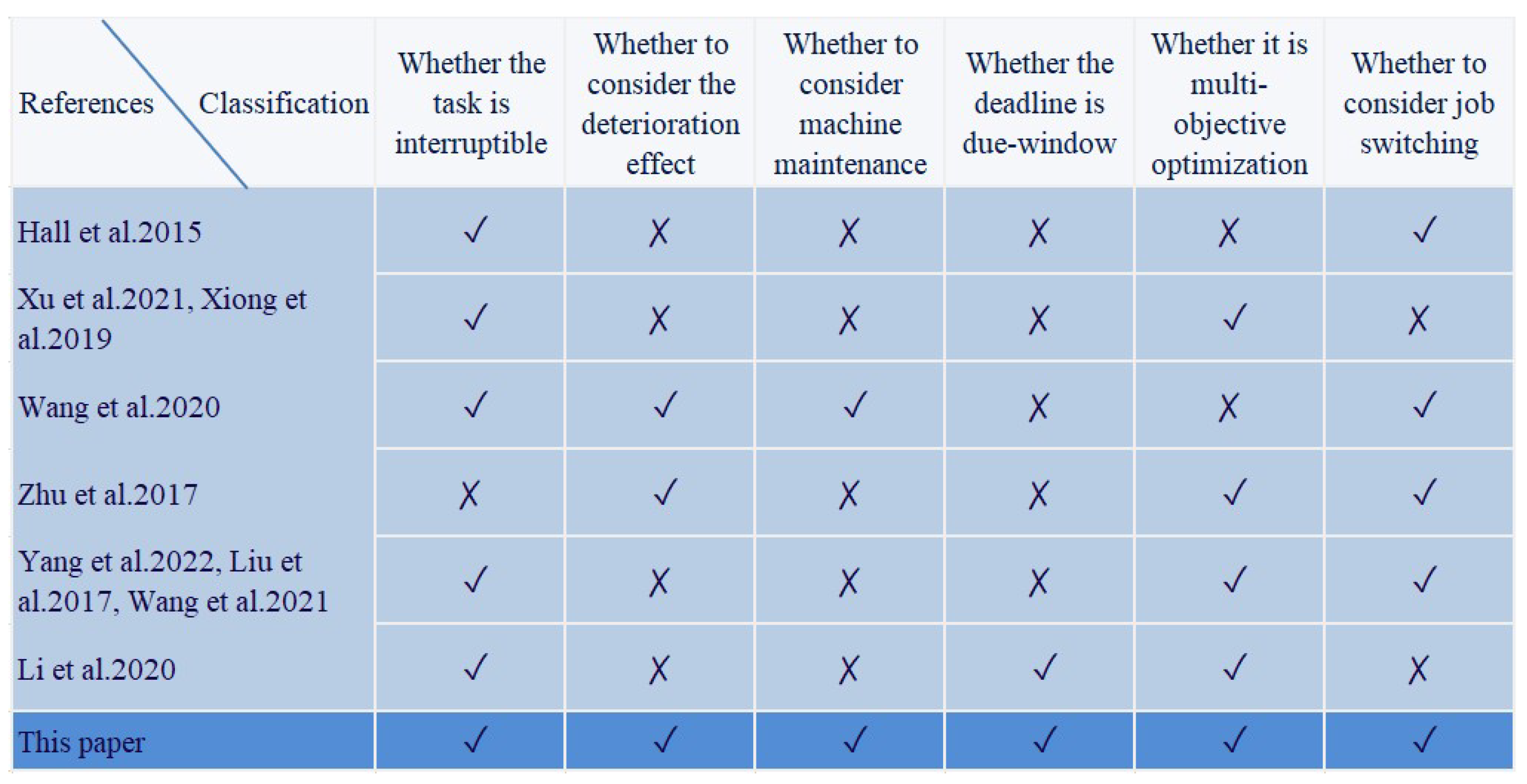
To provide a quick and comprehensive understanding of the latest research on multitasking scheduling problems, Table 1 below provides a clear overview of the key information from recent studies in this field.
Through a close examination of current studies, we have identified several key limitations. For instance, many studies treat due dates as constant values, rather than intervals, which may lead to insufficient flexibility in practical applications. Furthermore, the existing research often assumes that the tasks being processed are undisturbable, which can pose difficulties when handling emergency tasks or priority changes. Additionally, unlike machines, human operators experience decreased efficiency as working hours increase and require periodic rest. If a human operator fails to have sufficient rest, fatigue and illness may occur, necessitating longer recovery periods known as deteriorating maintenance. To address these limitations, this research paper aims to bridge the gap by considering scheduling while multitasking on a single machine, taking into account the effects of aging, deteriorating maintenance, and treating the due date as an interval, rather than a fixed point, allowing for greater flexibility and adaptability in real-world scenarios. In keeping with the nomenclature of traditional machine scheduling, we call the human operator a “machine”.
The contributions of the paper include the following: (i) We first studied the scheduling problem that introduced due-window assignments and deteriorating maintenance in a multitasking environment. (ii) A polynomial algorithm of complexity is proposed to solve this problem. (iii) We performed numerical studies to demonstrate that, with some combinations of parameters, multitasking is more efficient than non-multitasking.
To more intuitively demonstrate the positioning of our work within the field of job scheduling research, we designed a classification chart (see Figure 1). This chart highlights the unique combination of factors considered in our study, including due-window assignment, machine maintenance, and the optimization of multiple objectives such as time and cost. It further underscores our innovativeness in this domain.
This paper is organized as follows: In Section 2, we provide an overview and definition of the scheduling model under study, such as the multitasking scheduling environment. In Section 3, we propose a polynomial-time algorithm to solve the concerns mentioned and present a numerical instance to show how the approach works. In Section 4, experiments on the algorithm using randomly generated data are presented to assess the impact of the algorithm and compare the difference between multitasking and non-multitasking. The concluding section wraps up the paper and outlines potential avenues as topics for future exploration.
2. Problem Formulation
The topic in question can be formally delineated as follows: We possess a collection of n unrelated jobs, labeled as , that must be executed on a consistently operational machine commencing at time zero. Time zero marks the beginning of each work’s eligibility for processing, and the machine is capable of handling only a single job at any given moment. The time taken for the regular processing of job is denoted as , while the point in time when it is completed is represented with . In mathematics and many other fields, symmetry typically refers to a kind of invariance or consistency in which the properties or structure of an object or system remain unchanged when subjected to certain transformations. When a machine exhibits consistency in its performance and efficiency across different tasks, we say that this performance is symmetrical. In such cases, the machine’s performance and efficiency should not be influenced by the nature or scale of the tasks but should maintain symmetry, i.e., without any noticeable bias. However, due to the machine’s deterioration, the effective processing duration of job , denoted as , is determined using the formula , When scheduled in the location within a sequence, the aging factor is represented by . This factor takes into account the impact of aging on the machine’s efficiency during the processing of a specific job. Moreover, all jobs are bound by a common due-window within which it is highly preferable to accomplish their processing. In other words, the efficient processing of each job is crucial to achieving the overall completion objective. Let and stand for the initiation and termination times of the due-window, respectively, and signifies the span of the due-window. Both and , subsequently leading to D, are considered decision variables that are negotiated and agreed upon with the customer. It is important to stress that there are no penalties for jobs that are finished within the allotted time window. Nevertheless, if job is finished before the due-window’s start time, , it will face an earliness penalty, , which is determined by the degree of early completion. Here, we designate as the earliness of job . On the contrary, if task is not completed by the due-window’s ending time, , it will face a tardiness penalty, , which varies based on the degree of delay. In this case, we designate as the tardiness of job . These penalties are critical factors to consider when optimizing job scheduling within the due-window to achieve the most favorable outcomes for both the customer and the overall operation.
To lessen the effects of machine deterioration, an effective strategy involves executing a single machine maintenance operation within the planning period. By restoring the machine to its initial level of efficiency, this maintenance procedure enhances the machine’s overall performance. Consequently, upon the completion of the maintenance, if this is the initial job to begin processing on the designated machine, the real time it takes to process a job, , will match its regular processing time. Let us consider as the index corresponding to the first job scheduled after the maintenance operation. Consequently, the real time it takes to process a job, , positioned at the rth position after the maintenance, is expressed as follows: , if , and otherwise. Moreover, the length of the maintenance operation is dependent upon the time when it begins. In precise terms, the actual maintenance duration is defined as , where represents the normal maintenance time, and serves as the maintenance factor.
In a multitasking environment, similar to the findings in [5], processing a specific job may encounter interruptions from other unfinished jobs. The designated task is referred to as the “primary job”. On the other hand, tasks that have undergone partial processing due to being interrupted by other jobs but have not yet been fully completed are known as “waiting jobs”. It is forbidden to preempt a primary job unless it is interrupted by a waiting job. Consequently, one job finishes before another assumes the role of principal job. This implies that each task needs to be selected as the main task exactly once. The partial processing of a job that occurs during its interruption of other jobs does not require repetition.
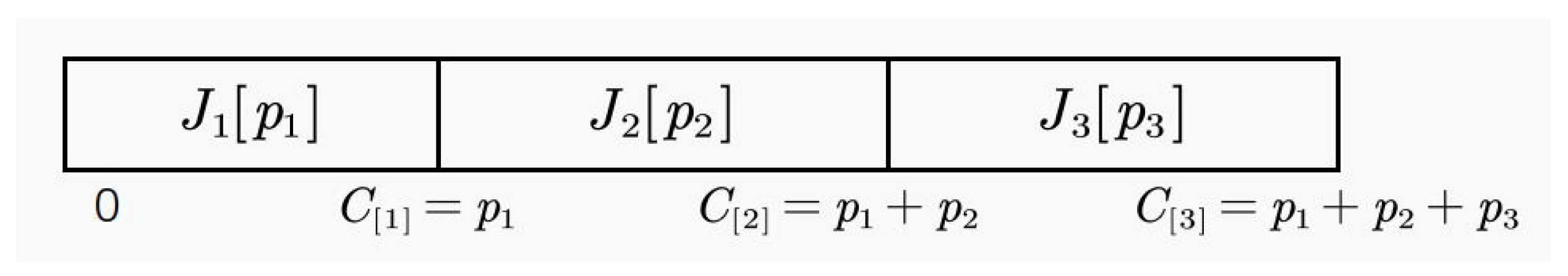
To more intuitively illustrate the importance of multitasking mechanisms and their differences from non-multitasking scheduling, we can use two diagrams for visual explanation and comparison. Assuming we have three Jobs to process, with their processing times denoted as , respectively, and represents the actual completion times for each job.
In Figure 2, once Job 1 begins processing, the system continues until this job is completed before moving on to Job 2, followed by Job 3. This approach does not allow for interruptions or task-switching during processing, so the overall completion time is the sum of the three individual task times.
In Figure 3, the actual completion time also needs to consider factors such as the overhead of job-switching, the time required for interruption-handling, and potential performance degradation due to increased machine runtime.
Assuming that job , where , is the rth primary job, we let be the set of corresponding waiting jobs and be the remaining normal processing time for any job, . The interruption time of job , which refers to the duration during which job interrupts job , is represented as , where
and . While processing the primary job, , an additional time, is incurred, representing the switching time for handling the interrupting jobs, with . Hence, the cumulative interruption duration throughout the processing of job is denoted as , where represents the aggregated time during which waiting jobs disrupt job .
Regarding the function , we introduce for to represent the residual normal processing duration of job following the interruption of r primary jobs. Thus, with . We postulate that is formulated in a manner such that remains positive for all values of and . This ensures that the residual processing duration of job is guaranteed to be positive whenever it assumes the role of the primary job, taking into account the switching time as well.
This study’s primary goal is to ascertain the following: (i) the optimal primary job sequence; (ii) the optimal due-window size and starting time; and (iii) the best moment to begin the maintenance process. The aim of this optimization is to minimize the cost function, Z, defined as the sum of , , , and over all jobs j from 1 to n. Here, , , , and are non-negative real numbers standing for penalties for early completion, tardiness, the beginning of the due-window, and its dimensions, respectively. Using the standard three-field notation for scheduling issues, we represent this optimization problem as , where denotes multitasking, represents maintenance operations, and indicates the processing time during multitasking.
3. Preliminary Analysis
This section aims to establish fundamental structural characteristics of optimal schedules. These characteristics will serve as the cornerstone for devising an effective algorithm to address the problem at hand.
Lemma 1.
The most effective schedule meeting the following conditions exists as follows:
(i) The jobs are completed without interruption starting at time zero;
(ii) The due-window’s start () and end () times are either set to zero or align with the completion periods of certain designated jobs.
Proof.
The proof for (i) is straightforward, as the problem’s objective function is regular, guaranteeing that it does not decrease with the completion periods of the jobs. The proof has a resemblance to Lemma 3 in [32]. □
Due to Lemma 1, we can concentrate on schedules that start from time 0 and do not include any idle periods. Consequently, we will only seek the optimal schedule among those where and are either set to 0 or correspond to the completion periods of specific jobs. Let and represent the indices and , respectively. The following Lemma indicates that the values of and are dependent on the cost parameters and remain unaffected by the positioning and magnitude of the maintenance endeavor.
Lemma 2.
There is a schedule that works well for the issue, in which the beginning time () and ending times () of the due-window are equivalent to and , respectively, where and
Proof.
The proof has a resemblance to Lemma 3 in [32]. □
Lemma 3.
Given and , two non-negative number sequences (for ), the sum of their corresponding element-wise products, denoted as , attains its minimum (maximum) value when the sequences are monotonically decreasing (increasing) in opposite (similar) directions.
Proof.
See page 261 in [33]. □
The variable is a binary flag indicating the assignment of job j to the rth location on the machine. If job j has been allocated to the rth position, takes the value of 1; otherwise, it remains at 0.
Consider an arbitrary but fixed job sequence, , that adheres to Lemma 3. For each job, in this sequence, where j ranges from 1 to n, let represent its completion periods, its earliness, and its tardiness. To formulate the expression for the completion periods of jobs , we need to examine three distinct cases.
Remark 1.
According to the proof process of Lemma 1 by Yang et al. [19], when , suppose that there exists a sequence about job j that starts at time zero and contains jobs at the th and th locations, such that the following applies: and Let The total cost can be formulated as where and They are comparable to the case of when the maintenance is carried out in the due-window (i.e., ) and when the maintenance is carried out after the due-window (i.e., ).
Case 1. , i.e., the maintenance operation, is implemented before the due-window. In this case, given , the remaining processing time of job is when job becomes a primary job since it has interrupted primary jobs. During the execution of the primary job , the switching time incurred by the jobs within the set amounts to . Additionally, the interruption time due to these jobs is determined via the sum . Consequently, the total time required to process job when it serves as the primary job is equal to , denoted as . As a consequence, the completion periods of jobs is determined as follows:
The following formula can be used to formulate the goal function:
Case 2. , the maintenance is in position , and it is implemented in the due-window. Thus,
The following formula can be used to formulate the goal function:
Case 3. , the maintenance, is in position and implemented after the due-window. Thus,
The following formula can be used to formulate the goal function:
Drawing upon the analysis above, we present the optimized Algorithm 1 that follows as a solution to the problem.
| Algorithm 1 Obtaining the Globally Optimal Sequence Based on Minimum Cost |
| Step 1. Referring to Lemma 2, identify the best locations for the due-window’s start time as and the finish time as . |
| Step 2. For y, execute from 1 to n. |
| Step 2.1. |
| Step 2.2. Perform for each j between 1 and n − 1. |
| Step 2.3. Compute the processing time using an equation with multitasking operations. |
| Step 3. Set |
| Step 4. Resolve the task allocation issue to derive a locally optimal schedule and determine the total cost associated with it. |
| Step 5. if then proceed to 4. Otherwise, proceed to step 6. |
| Step 6. The globally optimal sequence refers to the one that incurs the minimal cost associated with the assignment of due dates. |
4. Special Case
This is the case as in [5,19]; the aging factor for and the interruption function is , where , and then for . The actual durations taken for the processing of job that was scheduled as a primary job is determined via , for . Then, when , our objective function reduces to
where
when ,
where
when ,
where
Drawing upon the preceding analysis, we present the following optimized Algorithm 2 as a solution to the problem.
Below, we provide an example to demonstrate the Algorithm 2 for problem .
Example 1.
There are jobs. We let and The aging factor, basic maintenance time, and maintenance factor are and respectively, according to Lemma 2. We can calculate that and
| Algorithm 2 Globally Optimal Sequence with Job-Independent Aging and Minimum Cost |
| Step 1. Referring to Lemma 2, identify the best locations for the due-window’s start time as and the finish time as . |
| Step 2. For y, execute from 1 to n. |
| Step 2.1. |
| Step 2.2. Perform for each j between 1 and n − 1. |
| Step 2.3. Compute the processing time using an equation with multitasking operations. |
| Step 3. Set |
| Step 4. For calculate the |
| Step 5. Put the biggest job on the position with the lowest , the next job on the position with the next-smallest , and so on. Then, the most efficient sequence of jobs and the value of the function Z are obtained via Lemma 3. |
| Step 6. if proceed to 4. Otherwise, proceed to step 7. |
| Step 7. The globally optimal sequence is characterized by the lowest cost associated with due date assignments. |
The usual processing durations are based on Hall, Leung, and Li [5]. The interruption factor switching function is with the expression , and the actual durations taken for processing are as follows:
We will tackle each case individually now:
Case 1 ( the maintenance is implemented before the due-window)
According to (23), we have The times of the beginning and ending within the due-window framework are and , respectively. Via step 5 of Algorithm 2, we obtain the locally best job scheduling (4, 3, 2, 6, 7, 5, 1). The total solution in Case 1 is
Case 2 ( the maintenance is in position i and implemented in the due-window)
For , according to (25), we have The times of the beginning and ending within the due-window framework are and , respectively. Via step 5 of Algorithm 2, we obtain the locally best job scheduling (1, 6, 4, 5, 7, 2, 3). The total solution in Case 1 is For the locally best job scheduling is (1,6,7,4,5,2,3). The total solution in Case 1 is
Case 3 ( the maintenance is in position i, and it is implemented after the due-window)
For , we repeat the procedure as in the above case. Table 2 summarizes the results for each possible site for the maintenance operation.
As shown in Table 2, the optimal solution on a global scale is obtained in Case 3 for As described in Cases 1 and 2, we have , and the job sequence is (1, 6, 7, 4, 5, 2, 3). The total solution in Case 2 is
5. Numerical Results
During the subsequent numerical investigations, we first described the design of the experiments and then compared the cost between multitasking and non-multitasking for common due date assignment problems. In order to connect with previous studies and demonstrate the progress of this research, the design and parameter settings of the numerical experiments are similar to those in [5,29]. The numerical tests were conducted using the following parameter settings: The quantity of jobs was fixed at the set values of . The job-processing duration was created at random using the discrete uniform distribution . , and b were chosen randomly from the discrete uniform distribution . Assessing how distinct values of and c impact the multitasking cost, we chose the values from , , and , respectively. We used to represent the choice. Thus, we had eight situations: , , , , , , and . We generated 100 problem instances. Thereby, we tested a total of instances.
Consider Z and the optimal total cost obtained for the problem and respectively. Let “avg” represent the average quantity of over the 100 instances for each combination. If the quantity is negative, it means that multitasking produces value, whereas if it is positive it means that multitasking increases the cost. “Max” and “Min” represent the maximum and minimum of the quantity over 100 problem instances, respectively.
- In Table 3, we can see that when , the average percentage cost is negative; when , both the average and minimum percentage costs are negative.The negative values for both the average and minimum percentage costs shown in Table 3 indicate that, within these specific ranges of task quantities (n), the multitasking approach achieves cost savings compared to the classical method. Typically, in cost comparisons, the savings achieved via one method relative to another are expressed as a percentage. If the cost of the multitasking approach is lower than that of the classical method, this difference is represented as a negative percentage.When , the negative average percentage cost suggests that multitasking is generally more cost-effective and efficient than the classical method within this range of task quantities.The negative minimum cost further implies that, within the considered range of tasks, there exists at least one task combination or scenario where the cost of multitasking is lower than that of the classical approach. This also means that, if our goal is to find the most cost-saving task allocation strategy, the multitasking approach is a worthwhile option to consider.
- In Table 3, when , the average percentage cost and the minimum percentage cost will increase with the increase in the number of jobs amounts to n for all the combinations . This means that the larger the task volume, the higher the cost required for multitasking.
- In Table 3, when the values of Q and c are fixed (i.e., the interruption and maintenance factor), the average percentage cost will decrease with the increase in the a value; when the values of a and c are fixed (i.e., the aging and maintenance factor), the proportion of multitasking’s cost as a percentage will decrease with the value of Q increasing. For example, for the combinations and , when , the values of “Ave”, “Max”, and “Min” will decrease from to .
- When , we get the exact opposite of . In Table 4, the average percentage cost and the minimum percentage cost will decrease with the increase in the quantity of jobs amounting to n. This indicates that there are fewer than 20 jobs. In this case, multitasking is more effective.
- In Table 4, the value of a is fixed; . Then, as the c value increases, so do the minimum and average percentage costs. For example, for combinations and , when , the values of “Ave” and “Min” will increase from to . This indicates that, in this situation, as the number of job switches increases, the total cost of multitasking also increases accordingly.
Although this study has demonstrated the effectiveness of the algorithm under specific parameter settings, there are certain limitations. Specifically, variations in parameter settings during experiments may have an impact on the algorithm’s results. Due to the complexity of the parameter space, we were unable to conduct comprehensive tests on all possible parameter combinations. In future research, further exploration of the specific effects of different parameter settings on algorithm performance can provide more accurate guidance for practical applications.
6. Conclusions and Further Research
This work considered aging impacts and deteriorating maintenance while scheduling multitasking and due-window assignments on a single system. The aim was to minimize a specific objective function related to the completion times of jobs in a multitasking environment. Subsequently, we will compare the value of this objective function in this environment with that in a non-multitasking context in order to evaluate whether multitasking can lead to higher processing efficiency compared to non-multitasking scenarios. In the particular instance of this issue, we also get an algorithm with lower time complexity. In addition, We demonstrate how the suggested Algorithm 1 operates using a numerical example. The computational results show that, for the problem we studied, the effect of multitasking is superior to non-multitasking when the number of concurrent tasks, n, does not exceed 30.
Further research may focus on the following: (i) extending the model and algorithm we studied to parallel machines or other machine environments [34]; (ii) applying a heuristic approach rooted in the Genetic Algorithm (GA) to tackle the problem addressed in this paper [35]; and (iii) resource allocation scheduling problems [21].
Funding
This research was supported by financial grants from the National Natural Science Foundation of China (grant no. 12061082).
Data Availability Statement
Data are contained within the article.
Acknowledgments
I thank the editors and reviewers for their constructive comments.
Conflicts of Interest
The author declares no conflicts of interest.
References
- Merriam-Webster Online. Multitasking. Merriam-Webster, Incorporated. Available online: http://www.merriam-webster.com/dictionary/multitasking (accessed on 18 November 2014).
- O’Leary, K.J.; Liebovitz, D.M.; Baker, D.W. How hospitalists spend their time: Insights on efficiency and safety. J. Hosp. Med 2006, 1, 88–93. [Google Scholar] [CrossRef]
- Kc, D.S. Does multitasking improve performance? Evidence from the emergency department. Manuf. Serv. Oper. Manag. 2013, 16, 168–183. [Google Scholar] [CrossRef]
- Laxmisan, A.; Hakimzada, F.; Sayan, O.R.; Green, R.A.; Zhang, J.; Patel, V.L. The multitasking clinician: Decision-making and cognitive demand during and after team handoffs in emergency care. Int. J. Med. Inform. 2007, 76, 801–811. [Google Scholar] [CrossRef]
- Hall, N.G.; Leung, J.Y.T.; Li, C.L. The effects of multitasking on operations scheduling. Prod. Oper. Manag. 2015, 24, 1248–1265. [Google Scholar] [CrossRef]
- Graham, R.L.; Lawler, E.L.; Lenstra, J.K.; Kan, A.R. Optimization and approximation in deterministic sequencing and scheduling: A survey. Ann. Discret. Math. 1979, 5, 287–326. [Google Scholar]
- Salmon Farm. Guest Blogger on “I Don’t Have a Poor Attention Span! I’m Multitasking”.
- Singh, R.M.; Awasthi, L.K.; Sikka, G. Towards metaheuristic scheduling techniques in cloud and fog: An extensive taxonomic review. Acm Comput. Surv. 2022, 55, 1–43. [Google Scholar] [CrossRef]
- Alboaneen, D.; Tianfield, H.; Zhang, Y.; Pranggono, B. A metaheuristic method for joint task scheduling and virtual machine placement in cloud data centers. Future Gener. Comput. Syst. 2021, 115, 201–212. [Google Scholar] [CrossRef]
- Noguera, J.; Badia, R.M. Multitasking on reconfigurable architectures: Microarchitecture support and dynamic scheduling. Trans. Embed. Comput. Syst. 2004, 3, 385–406. [Google Scholar] [CrossRef]
- Appasami, G.; Suresh Joseph, K. Optimization of operating systems towards green computing. Int. J. Comb. Optim. Probl. Inform. 2011, 2, 39–51. [Google Scholar]
- Wang, W.; Ranka, S.; Mishra, P. Energy-aware dynamic slack allocation for real-time multitasking systems. Sustain. Comput. Inform. Syst. 2012, 2, 128–137. [Google Scholar] [CrossRef]
- Sachdeva, S.; Panwar, P. A review of multiprocessor-directed acyclic graph (DAG) scheduling algorithms. Int. J. Comput. Sci. Commun. 2015, 66, 67–72. [Google Scholar]
- Cheng, T.E. Optimal common due-date with limited completion time deviation. Comput. Oper. Res. 1988, 15, 91–96. [Google Scholar] [CrossRef]
- Liman, S.D.; Panwalkar, S.S.; Thongmee, S. Common due window size and location determination in a single machine scheduling problem. J. Oper. Res. Soc. 1998, 49, 1007–1010. [Google Scholar] [CrossRef]
- Huo, Y.; Miao, C.; Kong, F.; Zhang, Y. Multitasking scheduling with alternate periods. J. Comb. Optim. 2023, 45, 92. [Google Scholar] [CrossRef]
- Xu, C.; Xu, Y.; Zheng, F.; Liu, M. Multitasking scheduling problem with a common due-window. RAIRO—Oper. Res. 2021, 55, 1787–1798. [Google Scholar] [CrossRef]
- Mosheiov, G.; Sarig, A. Scheduling a maintenance activity and due-window assignment on a single machine. Comput. Oper. Res. 2009, 36, 2541–2545. [Google Scholar] [CrossRef]
- Yang, S.J.; Yang, D.L.; Cheng, T.C.E. Single-machine due-window assignment and scheduling with job-dependent aging effects and deteriorating maintenance. Comput. Oper. Res. 2010, 37, 1510–1514. [Google Scholar] [CrossRef]
- Yin, Y.; Wu, W.H.; Cheng, T.C.E.; Wu, C.C. Due-date assignment and single-machine scheduling with generalized position-dependent deteriorating jobs and deteriorating multi-maintenance activities. Int. J. Prod. Res. 2014, 52, 2311–2326. [Google Scholar] [CrossRef]
- Liu, L.; Wang, J.J.; Liu, F.; Liu, M. Single machine due window assignment and resource allocation scheduling problems with learning and general positional effects. J. Manuf. Syst. 2017, 43, 1–14. [Google Scholar] [CrossRef]
- Zhu, Z.; Zheng, F.; Chu, C. Multitasking scheduling problems with a rate-modifying activity. Int. J. Prod. Res. 2017, 55, 296–312. [Google Scholar] [CrossRef]
- Ji, M.; Zhang, W.; Liao, L.; Cheng, T.C.E.; Tan, Y. Multitasking parallel-machine scheduling with machine-dependent slack due-window assignment. Int. J. Prod. Res. 2019, 57, 1667–1684. [Google Scholar] [CrossRef]
- Xiong, X.; Zhou, P.; Yin, Y.; Cheng, T.C.E.; Li, D. An exact branch-and-price algorithm for multitasking scheduling on unrelated parallel machines. Nav. Res. Logist. (NRL) 2019, 66, 502–516. [Google Scholar] [CrossRef]
- Zhu, Z.; Liu, M.; Chu, C.; Li, J. Multitasking scheduling with multiple rate-modifying activities. Int. Trans. Oper. Res. 2019, 26, 1956–1976. [Google Scholar] [CrossRef]
- Yang, Y.; Yin, G.; Wang, C.; Yin, Y. Due date assignment and two-agent scheduling under a multitasking environment. J. Comb. Optim. 2022, 44, 2207–2223. [Google Scholar] [CrossRef]
- Wang, Y.; Wang, J.Q.; Yin, Y. Multitasking scheduling and due date assignment with deterioration effect and efficiency promotion. Comput. Ind. Eng. 2020, 146, 106569. [Google Scholar] [CrossRef]
- Zhu, Z.; Li, J.; Chu, C. Multitasking scheduling problems with deterioration effect. Math. Probl. Eng. 2017, 2017, 4750791. [Google Scholar] [CrossRef]
- Liu, M.; Wang, S.; Zheng, F.; Chu, C. Algorithms for the joint multitasking scheduling and common due date assignment problem. Int. J. Prod. Res. 2017, 55, 6052–6066. [Google Scholar] [CrossRef]
- Li, S.S.; Chen, R.X.; Tian, J. Multitasking scheduling problems with two competitive agents. Eng. Optim. 2020, 52, 1940–1956. [Google Scholar] [CrossRef]
- Wang, D.; Yu, Y.; Yin, Y.; Cheng, T.C.E. Multi-agent scheduling problems under multitasking. Int. J. Prod. Res. 2021, 59, 3633–3663. [Google Scholar] [CrossRef]
- Mosheiov, G.; Sidney, J.B. Scheduling a deteriorating maintenance activity on a single machine. J. Oper. Res. Soc. 2010, 61, 882–887. [Google Scholar] [CrossRef]
- Hardy, G.H.; Littlewood, J.E.; Pólya, G. Inequalities (Cambridge Mathematical Library); Cambridge University Press: Cambridge, UK, 1934. [Google Scholar]
- Yin, Y.; Wang, Y.; Cheng, T.C.E.; Liu, W.; Li, J. Parallel-machine scheduling of deteriorating jobs with potential machine disruptions. Omega 2017, 69, 17–28. [Google Scholar] [CrossRef]
- Asghari, M. Fuzzy programming for parallel machines scheduling: Minimizing weighted tardiness/earliness and flow time through genetic algorithm. J. Optim. Ind. Eng. 2014, 44, 61–73. [Google Scholar]

Figure 2.
Scheduling without multitasking.

Figure 3.
Scheduling with multitasking.


Table 1.
Summary of multitasking scheduling studies.
| Study | Use Case | Considerations | Optimization Tools |
|---|---|---|---|
| [5] | Single-machine multitasking scheduling | Impact of multitasking behavior on scheduling environment | Optimal algorithms |
| [23] | Parallel-machine multitasking scheduling with slack due-windows | Similar parallel machines | Scheduling algorithms with slack due windows |
| [24] | Multitasking scheduling on unrelated parallel machines | Minimizing total weighted completion time | Exact branch-and-price algorithm with inner and outer column generation |
| [25] | Extension to multiple rate-modifying activities (MRMAs) | Extending single RMA to multiple activities | Introduction of MRMA |
| [26] | Multi-agent multitasking scheduling with a common due date | Scheduling with multiple agents sharing a due date | Scheduling algorithms for multi-agent systems |
| [27] | Multitasking scheduling with position-dependent deterioration and rate improvement | Consideration of deterioration effects and upper bounds | Polynomial-time exact algorithms for given objectives |
Table 2.
The optimal sequences of jobs and their corresponding total costs for every conceivable placement of the MA.
Table 2.
The optimal sequences of jobs and their corresponding total costs for every conceivable placement of the MA.
| MA Position | Job Sequence | Total Cost | |
|---|---|---|---|
| 1 | (49.32, 92.80) | (4, 3, 2, 6, 7, 5, 1) | 14,140.17 |
| 2 | (28.29, 79.77) | (1, 6, 4, 5, 7, 2, 3) | 12,765.93 |
| 3 | (28.29, 70.17) | (1, 6, 7, 4, 5, 2, 3) | 12,078.68 |
| 4 | (30.05, 70.90) | (2, 5, 6, 7, 4, 1, 3) | 12,477.66 |
| 5 | (37.49, 81.26) | (1, 2, 5, 6, 7, 4, 3) | 14,087.38 |
| 6 | (38.36, 82.13) | (4, 1, 5, 7, 6, 2, 3) | 16,169.45 |
| 7 | (39.95, 83.72) | (3, 1, 5, 7, 6, 2, 4) | 17,731.70 |
Table 3.
The price of multitasking for issue .
| n | Ave | Max | Min | Ave | Max | Min | Ave | Max | Min | |||
|---|---|---|---|---|---|---|---|---|---|---|---|---|
| (0.15, 0.2, 0.1) | 10 | −10.39 | 13.57 | −31.66 | (0.15, 0.2, 0.3) | −8.56 | 18.07 | −44.71 | (0.15, 0.4, 0.1) | −6.43 | 14.67 | −34.09 |
| 20 | −13.04 | 0.63 | −37.00 | −14.79 | 3.32 | −41.82 | −11.86 | 0.50 | −30.85 | |||
| 30 | −9.26 | 8.08 | −33.75 | −7.51 | 8.85 | −31.34 | −8.05 | 5.59 | −29.84 | |||
| 50 | 12.65 | 30.46 | −8.80 | 12.65 | 31.79 | −6.52 | 15.08 | 28.23 | −9.15 | |||
| 70 | 40.47 | 55.00 | 25.08 | 39.33 | 55.43 | 24.98 | 44.05 | 57.40 | 24.54 | |||
| 90 | 70.07 | 85.31 | 51.42 | 69.42 | 92.46 | 49.33 | 73.23 | 89.12 | 56.82 | |||
| 100 | 85.40 | 111.53 | 63.37 | 83.17 | 102.45 | 57.96 | 89.20 | 115.97 | 67.37 | |||
| (0.15, 0.4, 0.3) | 10 | −9.04 | 14.54 | −35.45 | (0.25, 0.2, 0.1) | −29.10 | −8.45 | −53.32 | (0.25, 0.2, 0.3) | −25.85 | −7.13 | −55.52 |
| 20 | −12.88 | 2.33 | −36.79 | −30.65 | −16.02 | −54.41 | −30.74 | −11.88 | −52.04 | |||
| 30 | −6.79 | 8.32 | −24.13 | −21.61 | −1.58 | −46.63 | −21.49 | −6.25 | −38.86 | |||
| 50 | 14.29 | 28.19 | −1.70 | 2.74 | 18.29 | −13.27 | 1.42 | 20.47 | −13.15 | |||
| 70 | 41.75 | 62.67 | 21.99 | 31.52 | 49.08 | 13.26 | 31.43 | 47.32 | 12.66 | |||
| 90 | 73.56 | 87.66 | 59.00 | 62.15 | 84.98 | 38.67 | 61.89 | 78.64 | 44.79 | |||
| 100 | 86.50 | 106.85 | 64.64 | 79.25 | 97.38 | 60.46 | 78.53 | 104.72 | 63.29 | |||
| (0.25, 0.4, 0.1) | 10 | −27.30 | −7.84 | −53.10 | (0.25, 0.4, 0.3) | −27.48 | −7.38 | −55.67 | ||||
| 20 | −29.84 | −13.87 | −48.85 | −28.09 | −15.85 | −48.31 | ||||||
| 30 | −20.71 | −7.38 | −38.19 | −20.26 | −5.95 | −34.05 | ||||||
| 50 | 6.50 | 18.86 | −8.29 | 5.69 | 18.23 | −10.24 | ||||||
| 70 | 35.88 | 49.42 | 18.72 | 34.04 | 49.24 | 18.29 | ||||||
| 90 | 67.37 | 88.29 | 48.72 | 64.42 | 83.61 | 47.50 | ||||||
| 100 | 79.75 | 97.75 | 60.63 | 80.60 | 99.86 | 65.75 |
Table 4.
The price of multitasking for issue .
| n | Ave | Max | Min | Ave | Max | Min | Ave | Max | Min | |||
|---|---|---|---|---|---|---|---|---|---|---|---|---|
| (0.15, 0.2, 0.1) | 9 | −8.65 | 11.60 | −33.00 | (0.15, 0.2, 0.3) | −6.61 | 19.25 | −32.89 | (0.15, 0.4, 0.1) | −8.31 | 16.80 | −34.14 |
| 11 | −11.48 | 8.22 | −42.03 | −9.05 | 9.53 | −34.97 | −9.87 | 7.59 | −38.98 | |||
| 13 | −12.34 | 6.01 | −39.63 | −12.03 | 4.44 | −38.21 | −12.92 | 2.24 | −37.23 | |||
| 15 | −13.61 | 4.30 | −39.85 | −13.01 | 3.15 | −39.68 | −13.02 | 2.94 | −48.44 | |||
| 17 | −14.61 | 3.41 | −46.01 | −13.40 | 3.64 | −43.92 | −13.67 | 3.71 | −38.49 | |||
| 19 | −16.46 | 2.76 | −51.58 | −14.87 | 2.30 | −45.33 | −14.34 | 0.02 | −41.64 | |||
| 20 | −13.79 | 5.50 | −40.91 | −14.01 | 6.65 | −39.83 | −13.66 | 1.20 | −37.36 | |||
| (0.15, 0.4, 0.3) | 9 | −8.01 | 12.95 | −33.65 | (0.25, 0.2, 0.1) | −26.54 | −1.48 | −53.80 | (0.25, 0.2, 0.3) | −22.55 | 2.55 | −57.86 |
| 11 | −9.38 | 11.79 | −34.31 | −29.05 | −8.09 | −60.81 | −27.76 | −6.92 | −60.63 | |||
| 13 | −11.22 | 6.18 | −36.11 | −31.00 | −13.38 | −55.33 | −28.51 | −11.19 | −55.64 | |||
| 15 | −11.78 | 8.15 | −33.42 | −31.77 | −14.70 | −62.25 | −30.31 | −12.84 | −60.40 | |||
| 17 | −12.57 | 3.59 | −38.25 | −32.38 | −8.64 | −55.89 | −31.63 | −11.32 | −60.23 | |||
| 19 | −13.49 | −0.57 | −37.80 | −33.08 | −16.45 | −56.56 | −31.71 | −14.90 | −61.79 | |||
| 20 | −12.05 | 3.98 | −35.03 | −29.76 | −12.85 | −52.93 | −29.01 | −15.94 | −53.85 | |||
| (0.25, 0.4, 0.1) | 9 | −23.84 | −3.09 | −49.02 | (0.25, 0.4, 0.3) | −26.10 | −5.61 | −53.72 | ||||
| 11 | −27.88 | −7.88 | −60.76 | −28.64 | −10.69 | −55.51 | ||||||
| 13 | −29.98 | −7.85 | −55.17 | −29.22 | −12.21 | −58.03 | ||||||
| 15 | −30.48 | −17.64 | −54.68 | −30.41 | −11.23 | −54.73 | ||||||
| 17 | −30.92 | −16.19 | −53.31 | −31.30 | −15.66 | −55.38 | ||||||
| 19 | −31.83 | −17.54 | −53.96 | −31.58 | −14.95 | −53.89 | ||||||
| 20 | −29.58 | −12.18 | −53.21 | −29.40 | −13.28 | −51.23 |
Disclaimer/Publisher’s Note: The statements, opinions and data contained in all publications are solely those of the individual author(s) and contributor(s) and not of MDPI and/or the editor(s). MDPI and/or the editor(s) disclaim responsibility for any injury to people or property resulting from any ideas, methods, instructions or products referred to in the content. |
© 2024 by the author. Licensee MDPI, Basel, Switzerland. This article is an open access article distributed under the terms and conditions of the Creative Commons Attribution (CC BY) license (https://creativecommons.org/licenses/by/4.0/).
Share and Cite
MDPI and ACS Style
Zeng, L. An Exploration of Multitasking Scheduling Considering Interruptible Job Assignments, Machine Aging Effects, the Influence of Deteriorating Maintenance, and Symmetry. Symmetry 2024, 16, 380. https://doi.org/10.3390/sym16030380
AMA Style
Zeng L. An Exploration of Multitasking Scheduling Considering Interruptible Job Assignments, Machine Aging Effects, the Influence of Deteriorating Maintenance, and Symmetry. Symmetry. 2024; 16(3):380. https://doi.org/10.3390/sym16030380
Chicago/Turabian StyleZeng, Li. 2024. "An Exploration of Multitasking Scheduling Considering Interruptible Job Assignments, Machine Aging Effects, the Influence of Deteriorating Maintenance, and Symmetry" Symmetry 16, no. 3: 380. https://doi.org/10.3390/sym16030380
Note that from the first issue of 2016, this journal uses article numbers instead of page numbers. See further details here.