
Automatic Trajectory Determination in Automated Robotic Welding Considering Weld Joint Symmetry


1
Department of Engineering, Public University of Navarre, 31006 Pamplona, Spain
2
Basque Research and Technology Alliance (BRTA), TECNALIA, 20009 Donostia-San Sebastián, Spain
*
Author to whom correspondence should be addressed.
Symmetry 2023, 15(9), 1776; https://doi.org/10.3390/sym15091776
Submission received: 18 August 2023
/
Revised: 9 September 2023
/
Accepted: 15 September 2023
/
Published: 16 September 2023
(This article belongs to the Special Issue Advanced Materials, Structures, Symmetrical Design and Mechanism in Mechanical Engineering)
Abstract
:The field of inspection for welded structures is currently in a state of rapid transformation driven by a convergence of global technological, regulatory, and economic factors. This evolution is propelled by several key drivers, including the introduction of novel materials and welding processes, continuous advancements in inspection technologies, innovative approaches to weld acceptance code philosophy and certification procedures, growing demands for cost-effectiveness and production quality, and the imperative to extend the lifespan of aging structures. Foremost among the challenges faced by producers today is the imperative to meet customer demands, which entails addressing both their explicit and implicit needs. Furthermore, the integration of emerging materials and technologies necessitates the exploration of fresh solutions. These solutions aim to enhance inspection process efficiency while providing precise quantitative insights into defect identification and location. To this end, our project proposes cutting-edge technologies, some of which have yet to gain approval within the sector. Noteworthy among these innovations is the integration of vision systems into welding robots, among other solutions. This paper introduces a groundbreaking algorithm for tool path selection, leveraging profile scanning and the concept of joint symmetry. The application of symmetry principles for trajectory determination represents a pioneering approach within this expansive field.
1. Introduction
In heavy industry (shipping, Oil&Gas, energy…), structures are made up of hundreds of components joined by welding in relatively complex, heavy parts known as joints in different joint configurations. These complex joints are difficult to weld as they present: (i) non-uniform and irregular weld grooves; and (ii) weld positions that require special skills in the welding process. In addition, they pose great physical demand and risk to the welding operator. Current practice for manufacturing such thick and complex joint structures has been largely limited to hand welding processes. Welding automation with robotic arms has become an inevitable trend in modern manufacturing technologies. This process can be either automated by using “click and go”, where the robot will weld a line where the point was described, or by using an online tracking algorithm, where the robot will choose the point where to weld the line in every layer [1]. Intelligent welding is composed of three parts. First, the precise data acquisition by laser vision and the following data processing for an optimal torch location. Second, the accurate weld seam tracking for different weld joints. Third, real-time weld defect detection to see if the welding would pass quality control [2]. These processes are complex due to linearity and time variation. Other factors influence the welding. Laser reflection during welding is an issue caused by spectrum signals [3], arc sound signals [4], or molten pools [5], which can alter the scanned profile and be inaccurate. Another big issue to face is the similarity in the contraction the thick plates suffer as a result of the welding’s high temperature. That is why the method “click and go” can make mistakes unless the operator clicks where to weld in every layer of the scan, as the profile shape of the beginning point of welding and the last point of welding for the thick plate is completely different. The auto-selection of a point is an improvement for the process, as there is no need for an operator to select the point on each layer.
Several robotic welding configurations have been developed, some targeting the welding of large-diameter pipes to solve the problems of welding large, complex joint structures [6]. These provide a Computer Aid Design (CAD)-based framework in which the welding solution can be planned, modified, and simulated with the accurate robotic kinematics and ideal (nominal) dimensions of the workpiece before job execution (Chen et al.) [7]. Tsai et al. [8] developed a robotic arc welding offline programming system in which the workpieces and the welding step were represented by analytical geometries. Shi et al. [9,10] developed a single-step robotic path planning system for the welding of intersecting pipes using geometrical models of the pipes. Yang et al. [11] reported a vision-based approach to obtaining workpiece groove information for double-sided, double-arc, double-sided welding. Ahmed et al. [12] developed a de-coupled path planning approach for seam welding a joint from branch to seam, including robot paths to weld passes and intermediate robot paths without collisions between consecutive passes.
In terms of monitoring the geometrical qualities of the weld, one of the incentive factors was the inclusion of the welding solutions as a source of generation for additive manufacturing by wire. In these technologies, the inspection of the geometry of the weld that originates the layer is of great relevance [13]. Some of the work related to weld monitoring for the additive Ding et al. [14] employed a 3D laser scanner for bead height measurement and also determined the overlapping distance. The raw data of the weld bead profile were processed to obtain the geometrical characteristics. Karmuhilan et al. [15] also studied the bead height and width using the welding process parameters of the coordinate measuring machine (CMM) to control the bead geometry using an artificial neural network (ANN) model of the bead parameters. Venkatarao [16] studies a larger number of geometrical parameters, including weld bead depth, weld bead height, weld bead width, and weld pool width; the latter parameter is measured in-line as it is specific to the process stage, and a learning-based optimization technique was used to optimize the weld bead geometry, but its measurement was done off-line by microscopy to validate a finite element model. Artaza et al. [17] also employ microscopic image analysis for the study of total wall geometry. Wang et al. [18] made a detailed study of bead geometry with multiple variables, including penetration area, aspect ratio, and dilution ratio, seeking to optimize by using the response surface method and a Box–Behnken design and taking the process parameters in additive arc manufacturing as control variables.
Other papers that measure different geometrical values during welding, including arc strike area, arc extinction, bead width, bead height, penetration, and dilution, are [19,20,21]. Tang et al. [19] perform this using an infrared camera and an arial topography measurement sensor to avoid geometrical errors in the critical initial and final zones of the weld. Li et al. [20] employ a laser displacement scanner to control the variation of the welded layer geometry, taking into account the ratio between width and height. Sarathchandra et al. [21], on the other hand, employ a 3D optical microscope as a measurement sensor, processing the images with the open-source software ImageJ to obtain and train backward models that take as input the current, standoff distance, and weld speed to guarantee the quality of the weld bead.
Dinovitzer et al. [22] employ a machine-integrated laser profilometer to measure the seam, a sensor solution similar to the one proposed in this paper, seeking to adjust welding parameters such as travel speed and wire feed speed using the Taguchi method and an ANOVA analysis to determine the effects of these parameters on the geometry. Many of these approaches to geometry and trajectory management are of broad interest, but as far as the application of symmetry concepts is concerned, they remain in the observation of the phenomenon. As for the application of symmetry in melt pool measurement, process control, and geometry estimation, the paper presented by Veiga et al. [23] does consider symmetry as a method of process quality analysis.
This paper focuses on the planning and optimization of the robot movement for the torch trajectory to pass through the weld joint in the optimal deposition zone defined between the union of the two plates. In this document, a position search algorithm is adopted to optimize the robot movement that defines the determined welding pass to achieve a smooth movement of the torch that meets the requirements of the welding task, such as the kinematic capabilities of the welding machine. robot, that is, the accessibility of the robot and the consistency of the robot’s movement.
2. Materials and Methods
This section describes the hardware elements, the auxiliary elements, and the communication between the different systems that make up the solution.
2.1. Experimental Set-Up
The material to be welded is a mild steel plate prepared in joint for oil and gas applications. The welding wire used is a commercially available 1.6 mm diameter welding wire of ER70 welding steel. Process monitoring is carried out using an open-loop control system. For this purpose, a laser scanner has been installed as an external sensor, and the internal signals of the welding machine are collected: intensity, voltage, wire speed, and feed rate. The positions of the robot axes and the wrist angles concerning the workpiece coordinates are also monitored. A welding cell has been enabled, whose hardware (Figure 1) is composed of the following devices: (i) FANUC robot; (ii) welding machine: EWM ALPHA Q-532. BUSINTX11 Profibus interface; (iii) laser profilometer of Quelltech Q4-120 and a PC. Table 1 shows the characteristics of the laser scanner used.
The torch, inclined perpendicular to the joint, utilized the Gas Metal Arc Welding (GMAW) process. GMAW, commonly known as MIG (Metal Inert Gas) welding, is a widely employed welding technique in which a consumable electrode wire is continuously fed into the weld pool. The torch, set perpendicular to the joint, employed an 18 mm diameter nozzle with an 18 mm stick-out. As a shielding gas, we used a mixture comprising 80% argon (Ar) and 20% carbon dioxide (CO2) at a flow rate of 18 L/min. Figure 1 illustrates the setup of the various components of the welding equipment. Gas Metal Arc Welding (GMAW) is renowned for its versatility and efficiency in joining a wide range of materials, making it a popular choice across various industrial applications. It offers advantages such as precise control over the welding process, minimal spatter, and high deposition rates. In our study, we employed GMAW with the specific parameters mentioned above to attain precise and reliable welding results. In the experimental setup, we employed the Gas Metal Arc Welding (GMAW) technique with short-circuit transfer. The wire’s inclination was maintained in a neutral position. Short-circuit transfer is a method used when a lower voltage is applied in MIG welding.
The sheets are to be welded in prepared sheets with a double bevel joint on both sides, the front and the back. The total thickness of the plate is 60 mm with a 55-degree angle. The aim is to locate the nozzle in the area closest to the joint of the two sheets. Figure 2 shows the diagram described above and the actual part to be welded. The sheets are pre-assembled at the ends to ensure that deformations are minimized in the initial stages of welding.
Table 2 summarizes the welding process parameters. The paper aims to define the trajectory of the torch during the welding of the joint in the first layer based on the symmetry of the joint. The most relevant parameters shown for the definition of the algorithm described here are the nozzle diameter and the stick-out, which influence the position of the torch.
2.2. Data Acquisition Chain
To communicate the different elements that make up the welding chain, which are the robot, the monitoring application, the database, and the laser, a device-dependent communication system, has been established. As an initial phase in the application of the algorithm, a supervised welding system has been developed and installed. Its schematic representation can be seen in Figure 3. This system aims to produce welds automatically using a robotic system. In this system, process monitoring is carried out using an open-loop control system. For this purpose, a laser scanner has been installed as an external sensor, and the internal signals of the welding machine are collected: intensity, voltage, wire speed, and feed rate. The positions of the robot axes and the welding wrist angles concerning the workpiece coordinates are also monitored.
Before the first pass to seal the joint, a scanning sequence is performed. Figure 4 shows the 3D reconstruction of the joint based on the 2D profiles acquired by the laser profilometer. For each pass, six profiles of the section are stored and displayed on the screen for trajectory generation. With the six points supervised by the operator, the point is calculated and used as the robot’s starting point for the next section of the pass until the joint is completed.
Figure 5 shows the point clouds of the six discrete equidistant profiles recorded by the laser. So that they cover the 140 mm length of the joint. As can be seen in Figure 5, there are different sources of uncertainty when defining the trajectory. On the one hand, the point cloud may contain some brightness that is considered aberrant and has to be removed by filtering. The profiles show a misalignment that suggests that the joint is not aligned with the profilometric laser trajectory. The algorithm described in this paper will consider these difficulties, as well as possible misalignments of the sheet on the table, to show a robust solution.
3. Results
The results section describes the methodology used, starting from the treatment of the profile acquired by the laser profilometer, the determination of the welding point, the study of the joint symmetry, and finally its implication in the definition of the torch positions to carry out the welding process of the first layer.
3.1. Processing of Scanned Profiles
The objective of this task is to define the processing and preparation of the profiles captured by the laser sensor for the definition of the torch trajectory in welding geometry coupons. As described in Section 2.2, the profiles arrive at the algorithm as a cloud of (x, z) points. From all the acquired profiles, six profiles are discretized to generate the trajectory, taking into account the length of the final trajectory. These six profiles have been determined discretely because they establish a smooth trajectory for a joint that, in theoretical dimensions, is straight. The decision to discretize or divide the trajectory into six profiles was made by agreement, considering the total length of the coupon to be welded, which was 140 mm. This coupon was relatively short, and significant deviations from straightness were not expected. It is considered that the origin of the deviations will be due either to a bad positioning of the plates, a bad support, or a deformation once the plate is turned and the back side is accessed. Therefore, the treatment performed on the set of points (x, z) defining a unitary profile (Figure 6a) follows the following steps:
- (a)
- The profile is set to 0 (signal acquired in Figure 6a);
- (b)
- The intensity signal acquired by the profilometer is filtered using a phase 0 filter based on a moving median filter. Soft filtering of the signal to eliminate brightness in the profile, with an order N = 7 (see Figure 6b);
- (c)
- The area furthest away from the position sensor (Figure 6c) is calculated using a threshold. This will be defined in further detail in the next section.
This first treatment of the profiles aims to eliminate unwanted glare in the acquired signal due to poor cleaning of the lens filter, characteristics of the surface to be measured, glare from the finish, or impurities on the surface.
3.2. Determination of the Welding Point WP
The deposition conditions are the “trapezoidal rule”. When the grid spacing is non-uniform, it is not ruled out in the study of the symmetry of the bead in the longitudinal direction by analyzing the metallographic images under the microscope.
The objective is to find the index j where the two terms of the summation expressed in Equation (1) equal each other. Figure 7 shows the calculation of the AUC at the front and back joints. The vertical and horizontal lines show the cut of the graph where equal areas are found.
The AUC curve has a sigmoid function shape that allows us to describe its evolution. Its graph has a typical “S” shape. As can be seen, while the function of the obverse joint fits perfectly into this shape, the reverse side has a slope at the end of the function. This is explained by the deviation of the origin profile, which, as can be seen in Figure 8b, has a slight deformation. This means that the center-line does not perfectly describe the center of the trapezium to be filled. Therefore, to determine the center-point, a refinement of the calculation has been carried out. This refinement is based on the calculation of the crossing of the center-line with the profile (xcenter-line, zcenter-line). A threshold is then established where z > zcenter-line − 1. The midpoint of this region will be taken as the Welding Point (WP) (xcenter-point, zcenter-point), where to place the wire for welding. It can be seen in Figure 8b that in the case of the obverse joint, the two points are very close together, as the profiles resemble the theoretical model of the joint.
But as can be seen in Figure 8b, a correct estimation of the center point does not guarantee access to the joint without collision. For this reason, the angle of access of the nozzle to the welding point must be corrected, for which an algorithm based on the symmetry of the joint has been developed.
3.3. Symmetry Analysis
The approach to calculating the angle of attack of the flare is simple: we look for the angle where the symmetry of the joint is maximized. For the calculation of the symmetry, a similar approach has been used to that carried out by Veiga et al. [24] for the calculation of the symmetry in a zero weld bead, oriented in that case to additive manufacturing.
The function was taken, where z is the position of the point taken from the laser profilometer after filtering. The x corresponds to the other coordinates of the position. Therefore, is a discrete number of points in a continuous function for x in the range of the profilometer. Taking x = 0 as the position of the central point, calculated it as explained in Section 3.2. The above function can then be divided into the two sides of the joint whose symmetry we want to evaluate: the max(x) > x > 0 part and the min(x) < x < 0. In the following Figure 9, we will call them f(x) and f(−x), respectively, and take the length of the shorter part (a minimum of |max(x)| and |min(x)|). From this division of the function, we can calculate the symmetry function and the antisymmetry function by following the equation below:
It is normal to think that the asymmetric and symmetric functions will be influenced by a change in the coordinates derived from the rotation of the profile. This rotation is done by applying the generalized equation:
where x0 and z0 are the coordinates of the WP. The symmetry and antisymmetry functions are therefore evaluated for the profile rotated around the welding point at different angles of rotation, with θ being the established limit of the possible ones between −15 degrees and 15 degrees, with an increment of 0.5 degrees. Figure 9a,d below show the values at angles 10 degrees away from the origin for the back joint. At the origin, Figure 9b, the joint is in a relatively high symmetry position, but this positioning could cause collisions in the nozzle as it approaches. The optimum angle for nozzle angular positioning is 3 degrees, as seen in Figure 9c.
It could then be assumed that when the asymmetric function is closer to zero and the symmetric function is closer to the original functions, the function is more symmetric concerning the point of analysis. This assumption is transformed into a mathematical expression, creating a pair of coefficients that characterize this statement. These coefficients are S and C. They are calculated as follows:
Figure 10 shows the value of the coefficients S and C as a function of the angle of rotation θ, this angle being complementary to the angle of approach of the nozzle. S = 1 and C = 1, being pure symmetry, and C = 0 and S = −1 being anti-symmetry. Figure 10a shows how, for the front face, the maximum symmetry is given at 0 degrees, with no rotation being necessary at least in profile 0. On the other hand, in the case of the back joint, compensation is necessary. Figure 10b shows how the positive angles improve the nozzle’s symmetry and therefore the WP’s access. The optimum access angle is 3 degrees in the case of profile 0 at the back joint.
3.4. Automatic Trajectory Determination
In this section, the process of automatic trajectory determination is discussed. This process begins once the positions of the welding point and the angles of attack of the nozzle are known. Table 3 summarizes the different values and provides the observed coefficients. An excessively anomalous value of symmetry could correspond to a badly acquired profile or some obstacle in the generation of the trajectory. This key feature could be useful for the control of non-optimal set-up and clamping conditions.
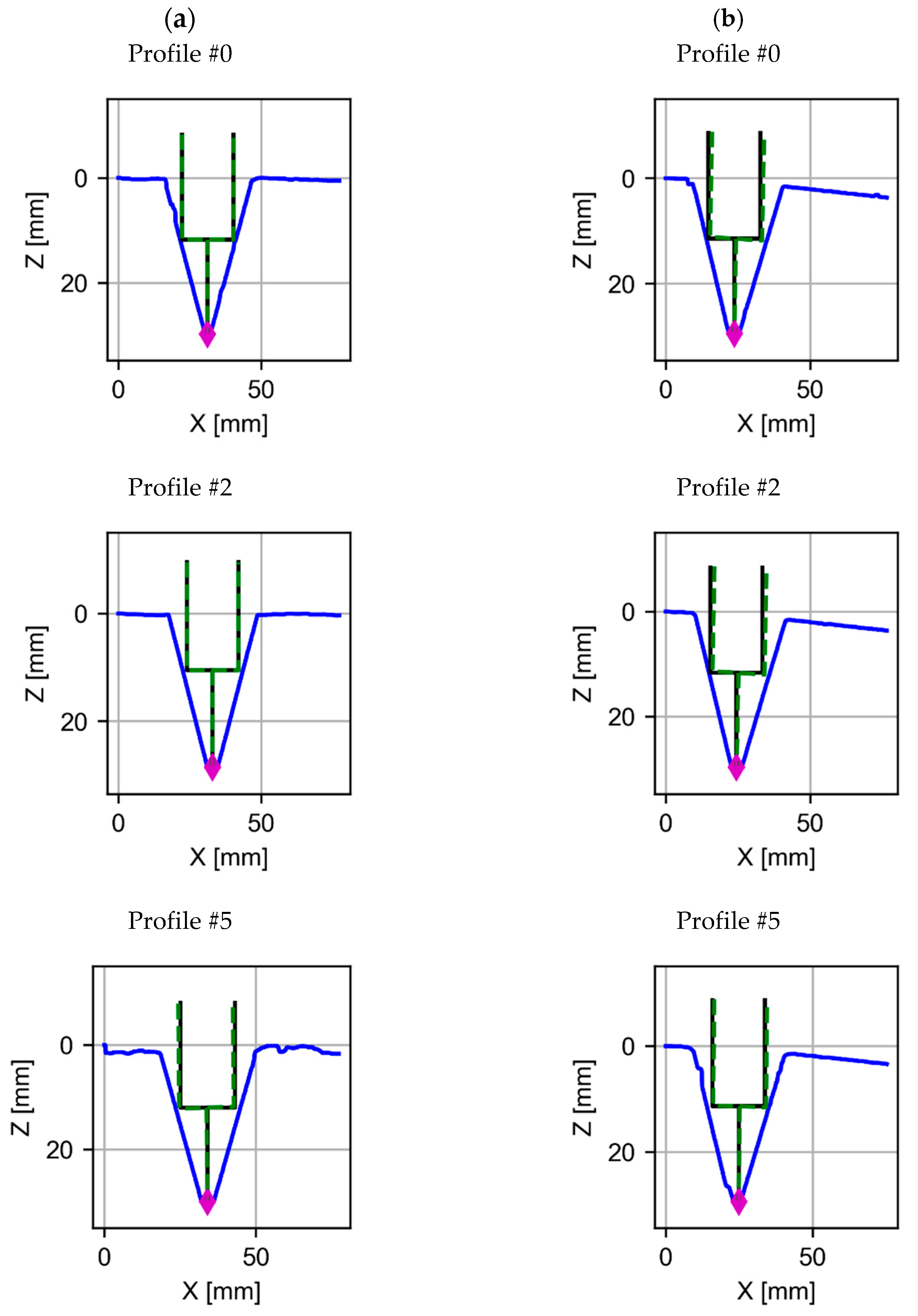
With these positions and angles, a representation of the nozzle position can be made considering its 18 mm diameter and the 18 mm stick-out. In the back joint, it can be seen how the occurrence of collisions is released. Figure 11 shows an example of three nozzle positions: the initial, the final, and an intermediate position on both sides of the joint.
These points generate the trajectory to be covered between the different points of the joint. As for the generation of the trajectory, the need for a fixed number of intervals or flexible and optimized intervals could be analyzed.
4. Conclusions
This paper presents a methodology for the automated welding of symmetrical joints. The main conclusions drawn from this study are as follows:
- A welding cell has been enabled where both robot position, welding parameters, and the geometry of the joint acquired by the laser profilometer have been monitored;
- A simple pre-processing of the profiles extracted from the profilometric laser measurement has been carried out. Six discrete profiles have been selected for each of the faces to be welded. The front side and the back side of the joint. This treatment eliminates aberrant spots due to surface impurities or shiny spots;
- The welding point has been selected based on the analysis of the curve under the profile to be welded. Finally, the calculation has been refined by using a threshold to better define the center point of the joint;
- To determine the angle of attack of the welding arc, a study of the joint symmetry as a function of the rotation of the profile was carried out. An offset close to 0 degrees on the front side and around 3 degrees on the back side has been defined;
- The joint shows symmetry close to pure symmetry, close to the theoretical model of the joint to be welded, with a C coefficient value greater than 0.998. An excessively low value of the symmetry value would mean a failure in the reading, either due to bad acquisition or bad assembly of the joint.
Future lines would be oriented toward the application of these algorithms for the definition of the trajectories not only in the welding of the first bead but also in other processes such as additive manufacturing by arc welding.
Author Contributions
Conceptualization, F.V., A.S. and E.A.; Data curation, F.V., P.V. and E.A.; Formal analysis, F.V., D.C. and E.A.; Investigation, F.V., A.S. and E.A.; Methodology, F.V., D.C. and E.A.; Project administration, A.S.; Supervision, A.S.; Validation, D.C., P.V. and A.S.; Writing—original draft, F.V. and D.C.; Writing—review and editing, F.V., D.C., P.V., A.S. and E.A. All authors have read and agreed to the published version of the manuscript.
Funding
This research received no external funding.
Institutional Review Board Statement
Not applicable.
Informed Consent Statement
Not applicable.
Data Availability Statement
The data presented in this study are available on request from the corresponding author.
Conflicts of Interest
The authors declare no conflict of interest.
References
- Ye, G.; Guo, J.; Sun, Z.; Li, C.; Zhong, S. Weld bead recognition using laser vision with model-based classification. Robot Comput. Integr. Manuf. 2018, 52, 9–16. [Google Scholar] [CrossRef]
- Sreeraj, P.; Kannan, T.; Maji, S. Prediction and control of weld bead geometry in gas metal arc welding process using genetic algorithm. Int. J. Mech. Prod. Eng. Res. Dev. 2013, 3, 143–154. [Google Scholar]
- He, Y.; Chen, Y.; Xu, Y.; Huang, Y.; Chen, S. Autonomous detection of weld seam profiles via a model of saliency-based visual attention for robotic arc welding. J. Intell. Robot. Syst. 2015, 81, 4–8. [Google Scholar] [CrossRef]
- Zhang, Z.F.; Yu, H.W.; Lv, N.; Chen, S.B. Real-time defect detection in pulsed GTAW of Al alloys trough online spectroscopy. J. Mater. Process. Technol. 2013, 212, 1145–1156. [Google Scholar]
- Lv, N.; Xu, Y.I.; Zhang, Z.F.; Wang, J.F.; Chen, B.; Chem, S.B. Audio sensing and modeling of and arc dynamic characteristic during pulsed al alloy GTAW process. Sens. Rev. 2013, 33, 141–156. [Google Scholar] [CrossRef]
- Yan, S.J.; Ong, S.K.; Nee, A.Y.C. Optimal pass planning for robotic welding of large-dimension joints with deep grooves. In Proceedings of the 9th International Conference on Digital Enterprise Technology (DET2016)—Intelligent Manufacturing in the Knowledge Economy Era, Nanjing, China, 29–31 March 2016. [Google Scholar]
- Chen, C.L.; Hu, S.S.; He, D.L.; Shen, J.Q. An approach to the path planning of tube–sphere intersection welds with the robot dedicated to J-groove joints. Robot. Comput. Integr. Manuf. 2013, 29, 41–48. [Google Scholar] [CrossRef]
- Tsai, M.J.; Lin, S.D.; Chen, M.C. Mathematical model for robotic arc-welding off-line programming system. Int. J. Comput. Integr. Manuf. 1992, 5, 300–309. [Google Scholar] [CrossRef]
- Shi, L.; Tian, X.C. Automation of main pipe-rotating welding scheme for intersecting pipes. Int. J. Adv. Manuf. Technol. 2015, 77, 955–964. [Google Scholar] [CrossRef]
- Shi, L.; Tian, X.C.; Zhang, C.H. Automatic programming for industrial robot to weld intersecting pipes. Int. J. Adv. Manuf. Technol. 2015, 81, 2099–2107. [Google Scholar] [CrossRef]
- Yang, C.D.; Ye, Z.; Chen, Y.X.; Zhong, J.Y.; Chen, S.B. Multi-pass path planning for thick plate by DSAW based on vision sensor. Sens. Rev. 2014, 34, 416–423. [Google Scholar] [CrossRef]
- Ahmed, S.M.; Yuan, J.Q.; Wu, Y.; Chew, C.M.; Pang, C.K. Collision-free path planning for multi-pass robotic welding. In Proceedings of the 2015 IEEE 20th Conference on Emerging Technologies and Factory Automation, Luxembourg, 8–11 September 2015. [Google Scholar]
- Xiong, J.; Zhang, K. Monitoring Multiple Geometrical Dimensions in WAAM Based on a Multi-Channel Monocular Visual Sensor. Measurement 2022, 204, 112097. [Google Scholar] [CrossRef]
- Ding, D.; He, F.; Yuan, L.; Pan, Z.; Wang, L.; Ros, M. The first step towards intelligent wire arc additive manufacturing: An automatic bead modelling system using machine learning through industrial information integration. J. Ind. Inf. Integr. 2021, 23, 100218. [Google Scholar] [CrossRef]
- Karmuhilan, M.; Sood, A.K. Intelligent process model for bead geometry prediction in WAAM. Mater. Today Proc. 2018, 5, 24005–24013. [Google Scholar] [CrossRef]
- Venkatarao, K. The use of teaching-learning based optimization technique for optimizing weld bead geometry as well as power consumption in additive manufacturing. J. Clean. Prod. 2021, 279, 123891. [Google Scholar] [CrossRef]
- Artaza, T.; Suárez, A.; Veiga, F.; Braceras, I.; Tabernero, I.; Larrañaga, O.; Lamikiz, A. Wire Arc Additive Manufacturing Ti6Al4V Aeronautical Parts Using Plasma Arc Welding: Analysis of Heat-Treatment Processes in Different Atmospheres. J. Mater. Res. Technol. 2020, 9, 15454–15466. [Google Scholar] [CrossRef]
- Wang, C.; Bai, H.; Ren, C.; Fang, X.; Lu, B. A Comprehensive Prediction Model of Bead Geometry in Wire and Arc Additive Manufacturing. J. Phys. Conf. Ser. 2020, 1624, 022018. [Google Scholar] [CrossRef]
- Tang, S.; Guilan Wang, C.H.; Zhang, H. Investigation and control of weld bead ar both ends in WAAM. In Proceedings of the 30th Annual InternationalSolid Freeform Fabrication Symposium and Additive Manufacturing Conference, Austin, TX, USA, 12–14 August 2019. [Google Scholar]
- Li, F.; Chen, S.; Shi, J.; Zhao, Y.; Tian, H. Thermoelectric Cooling-Aided Bead Geometry Regulation in Wire and Arc-Based Additive Manufacturing of Thin-Walled Structures. Appl. Sci. 2018, 8, 207. [Google Scholar] [CrossRef]
- Sarathchandra, D.; Davidson, M.J.; Visvanathan, G. Parameters effect on SS304 beads deposited by wire arc additive manufacturing. Mater. Manuf. Process. 2020, 35, 852–858. [Google Scholar] [CrossRef]
- Dinovitzer, M.; Chen, X.; Laliberte, J.; Huang, X.; Frei, H. Effect of wire and arc additive manufacturing (WAAM) process parameters on bead geometry and microstructure. Addit. Manuf. 2019, 26, 138–146. [Google Scholar] [CrossRef]
- Veiga, F.; Suarez, A.; Aldalur, E.; Artaza, T. Wire Arc Additive Manufacturing of Invar Parts: Bead Geometry and Melt Pool Monitoring. Measurement 2022, 189, 110452. [Google Scholar] [CrossRef]
- Veiga, F.; Suárez, A.; Aldalur, E.; Bhujangrao, T. Effect of the Metal Transfer Mode on the Symmetry of Bead Geometry in WAAM Aluminum. Symmetry 2021, 13, 1245. [Google Scholar] [CrossRef]
Figure 1.
Experimental setup for robotic welding.
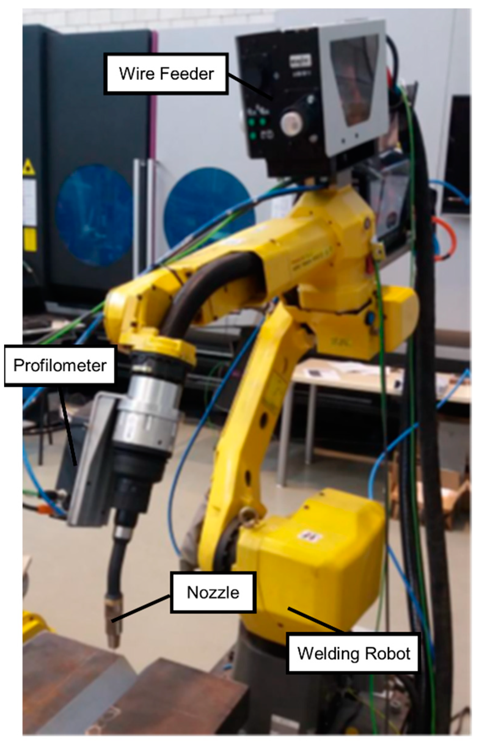
Figure 2.
Diagram of the case studies analyzed: (a) V-geometry and (b) real part.
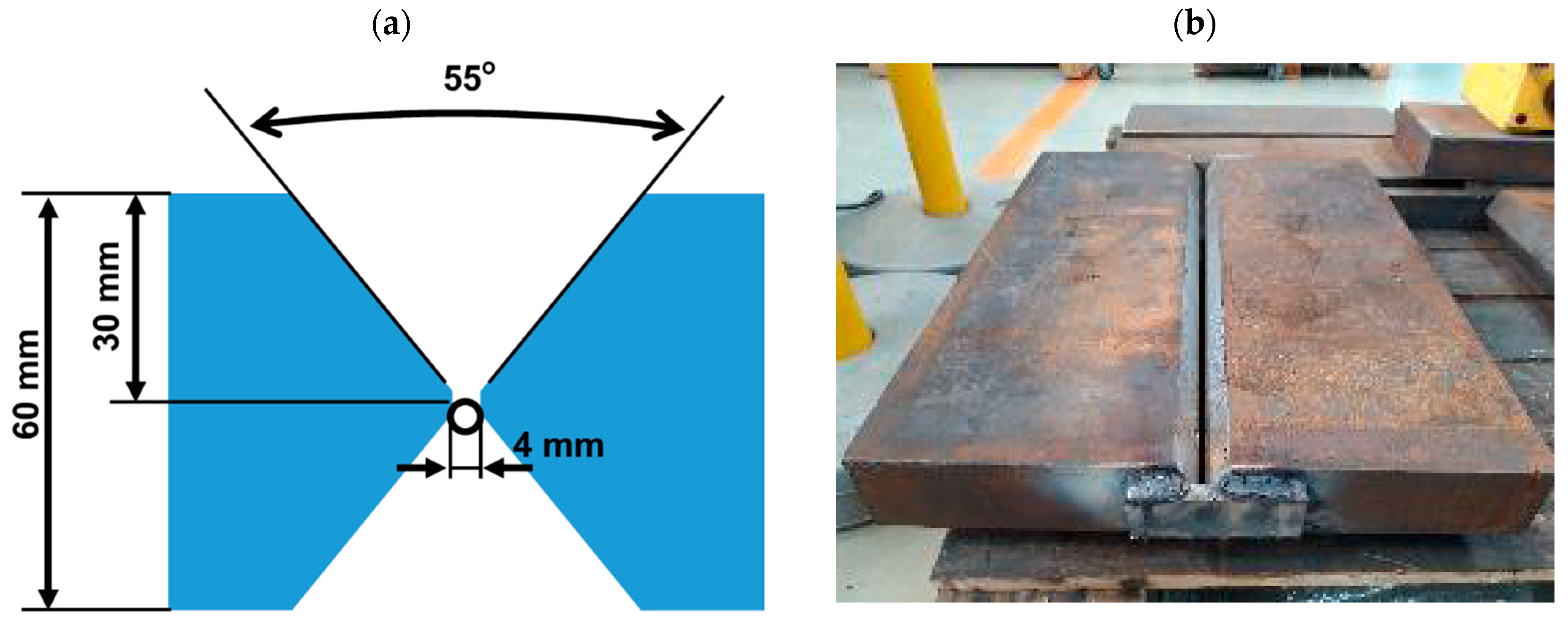
Figure 3.
Schematic representation of the system and its communications.

Figure 4.
Three-dimensional representation of the profiles with reconstruction of the welding joint.
Figure 4.
Three-dimensional representation of the profiles with reconstruction of the welding joint.
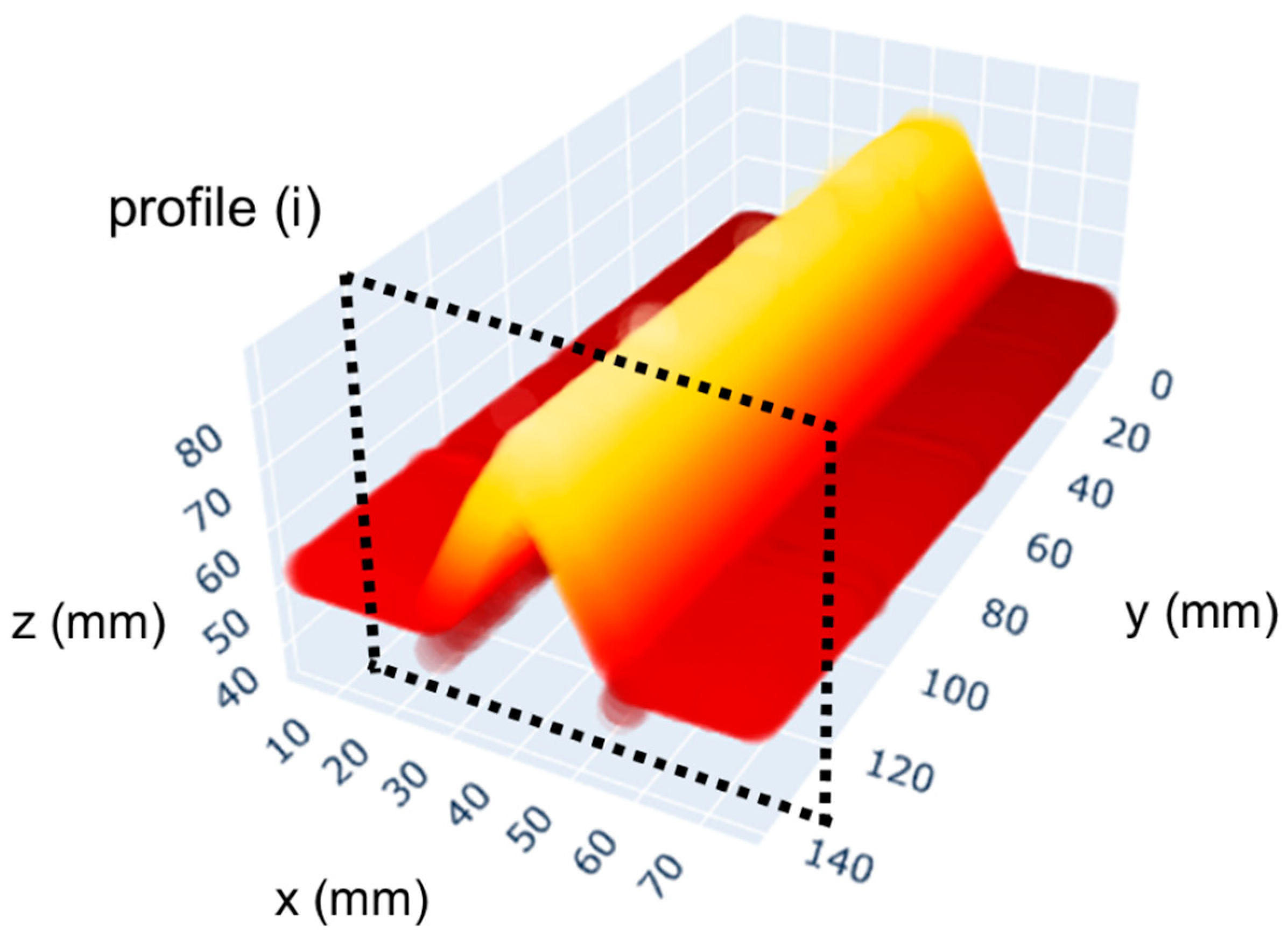
Figure 5.
Profiles acquired by the laser as a raw set of points.

Figure 6.
Stages in the processing of the laser-measured profile: (a) acquired raw weld seam; (b) filtered profile with moving median; (c) filtered profile with the weld spot area highlighted.
Figure 6.
Stages in the processing of the laser-measured profile: (a) acquired raw weld seam; (b) filtered profile with moving median; (c) filtered profile with the weld spot area highlighted.

Figure 7.
Area under the curve of the weld, with the line marking the middle area for (a) the front joint and (b) the back joint.
Figure 7.
Area under the curve of the weld, with the line marking the middle area for (a) the front joint and (b) the back joint.
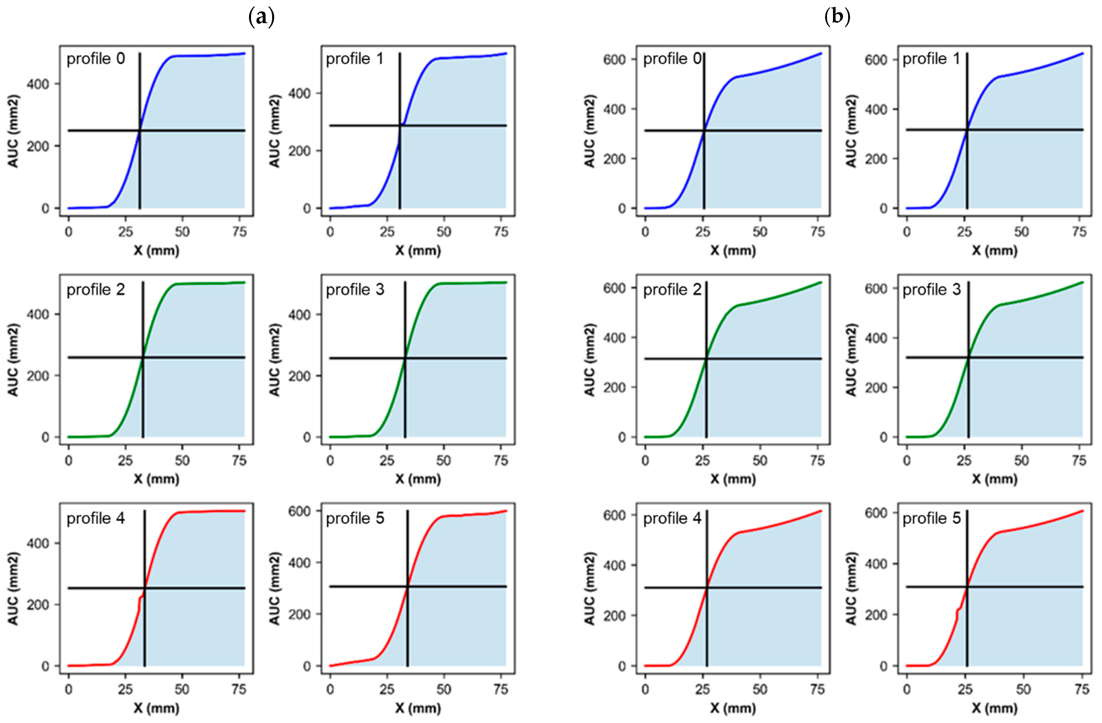
Figure 8.
Weld joint on (a) front joint and (b) back joint. The center-line is in the middle area and the calculated centerpoint is at the midpoint of the weld point.
Figure 8.
Weld joint on (a) front joint and (b) back joint. The center-line is in the middle area and the calculated centerpoint is at the midpoint of the weld point.

Figure 9.
functions to evaluate and symmetric antisymmetric functions at different angles of rotation: (a) −10 deg, (b) 0 deg, (c) 3 deg, and (d) 10 deg.
Figure 9.
functions to evaluate and symmetric antisymmetric functions at different angles of rotation: (a) −10 deg, (b) 0 deg, (c) 3 deg, and (d) 10 deg.

Figure 10.
Result of symmetric ratio (S) and correlation coefficient (C) evolution at different angles of rotation in profile 0 of (a) the front joint and (b) the back joint.
Figure 10.
Result of symmetric ratio (S) and correlation coefficient (C) evolution at different angles of rotation in profile 0 of (a) the front joint and (b) the back joint.
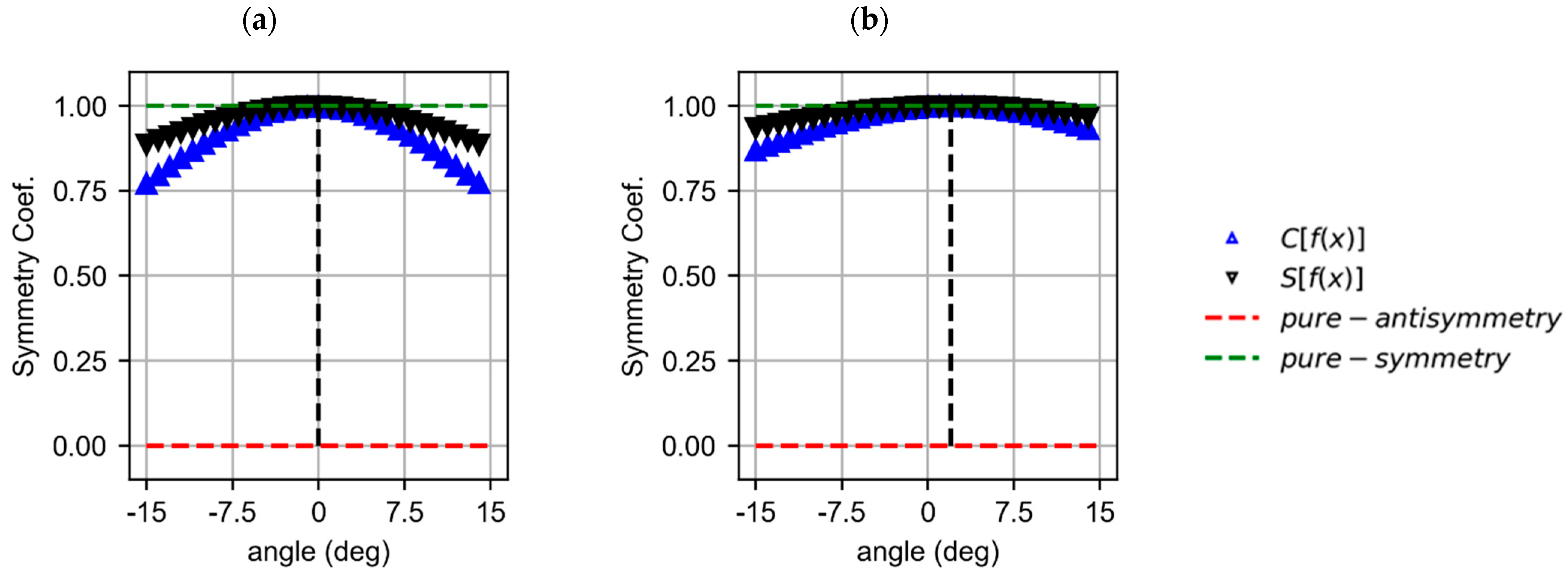
Figure 11.
Position and rotation of the nozzle in the different discrete profiles (#0, #2, and #5) at (a) the front joint and (b) the back joint.
Figure 11.
Position and rotation of the nozzle in the different discrete profiles (#0, #2, and #5) at (a) the front joint and (b) the back joint.

Table 1.
Characteristics of the Quelltech Q4-120 laser profilometer.
| Z-Range [mm] | X-Range [mm] | Distance [mm] | Resolution [mm] | Start Range X | End Range X | Dimensions [mm] | Weight [g] |
|---|---|---|---|---|---|---|---|
| 120 | 70 | 84 | 0.0798 | 60 | 80 | 186 × 32 × 84 | 430 |
Table 2.
Relevant parameters for the welding process.
| Nozzle Diameter (mm) | Stick-Out (mm) | Traverse Speed (cm/min) | Wire Feed (cm/min) | Voltage (V) | Current (A) |
|---|---|---|---|---|---|
| 18 | 18 | 42 | 920 | 32 | 280 |
Table 3.
Position and parameters obtained from the different profiles.
| Joint Side | Coord. xWP | Coord. zWP | C | S | |
|---|---|---|---|---|---|
| Front Joint Profile 0 | 31.182 | 29.766 | 0.9981 | 0.999 | −0.375 |
| Front Joint Profile 1 | 31.738 | 28.799 | 0.9997 | 0.9998 | −0.375 |
| Front Joint Profile 2 | 32.627 | 28.447 | 0.9994 | 0.9997 | −0.375 |
| Front Joint Profile 3 | 32.949 | 28.506 | 0.9983 | 0.9991 | −0.375 |
| Front Joint Profile 4 | 33.848 | 28.564 | 0.9987 | 0.9994 | −0.375 |
| Front Joint Profile 5 | 33.984 | 30 | 0.9992 | 0.9996 | −1.125 |
| Back Joint Profile 0 | 23.672 | 29.473 | 0.9991 | 0.9996 | 2.25 |
| Back Joint Profile 1 | 23.945 | 29.678 | 0.9995 | 0.9998 | 2.625 |
| Back Joint Profile 2 | 24.648 | 28.799 | 0.9982 | 0.9991 | 1.875 |
| Back Joint Profile 3 | 24.521 | 29.678 | 0.9995 | 0.9998 | 2.625 |
| Back Joint Profile 4 | 24.795 | 29.443 | 0.99865 | 0.9993 | 3 |
| Back Joint Profile 5 | 24.805 | 29.385 | 0.99647 | 0.9982 | 1.125 |
Disclaimer/Publisher’s Note: The statements, opinions and data contained in all publications are solely those of the individual author(s) and contributor(s) and not of MDPI and/or the editor(s). MDPI and/or the editor(s) disclaim responsibility for any injury to people or property resulting from any ideas, methods, instructions or products referred to in the content. |
© 2023 by the authors. Licensee MDPI, Basel, Switzerland. This article is an open access article distributed under the terms and conditions of the Creative Commons Attribution (CC BY) license (https://creativecommons.org/licenses/by/4.0/).
Share and Cite
MDPI and ACS Style
Curiel, D.; Veiga, F.; Suarez, A.; Villanueva, P.; Aldalur, E. Automatic Trajectory Determination in Automated Robotic Welding Considering Weld Joint Symmetry. Symmetry 2023, 15, 1776. https://doi.org/10.3390/sym15091776
AMA Style
Curiel D, Veiga F, Suarez A, Villanueva P, Aldalur E. Automatic Trajectory Determination in Automated Robotic Welding Considering Weld Joint Symmetry. Symmetry. 2023; 15(9):1776. https://doi.org/10.3390/sym15091776
Chicago/Turabian StyleCuriel, David, Fernando Veiga, Alfredo Suarez, Pedro Villanueva, and Eider Aldalur. 2023. "Automatic Trajectory Determination in Automated Robotic Welding Considering Weld Joint Symmetry" Symmetry 15, no. 9: 1776. https://doi.org/10.3390/sym15091776
Note that from the first issue of 2016, this journal uses article numbers instead of page numbers. See further details here.