
Generation of Stable Entanglement in an Optomechanical System with Dissipative Environment: Linear-and-Quadratic Couplings


Optics and Laser Group, Faculty of Physics, Yazd University, Yazd P.O. Box 89195-741, Iran
*
Author to whom correspondence should be addressed.
Symmetry 2023, 15(9), 1770; https://doi.org/10.3390/sym15091770
Submission received: 12 August 2023
/
Revised: 12 September 2023
/
Accepted: 13 September 2023
/
Published: 15 September 2023
(This article belongs to the Special Issue Quantum Entanglement and Quantum Optics: Latest Advances and Prospects)
Abstract
:In this paper, we present a theoretical scheme for the generation and manipulation of bipartite atom–atom entanglement in a dissipative optomechanical system containing two atoms in the presence of linear and nonlinear (quadratic) couplings. To achieve the goal of paper, we first obtain the interaction Hamiltonian in the interaction picture, and then, by considering some resonance conditions and applying the rotating wave approximation, the effective Hamiltonian, which is independent of time, is derived. In the continuation, the system solution was obtained via solving the Lindblad master equation, which includes atomic, optical and mechanical dissipation effects. Finally, bipartite atom–atom entanglement is quantitatively discussed, by evaluating the negativity, which is a well-known measure of entanglement. Our numerical simulations show that a significant degree of entanglement can be reached via adjusting the system parameters. It is noticeable that the optical and mechanical decay rates play an important role in the quasi-stability and even stability of the obtained atom–atom entanglement.
1. Introduction
Quantum entanglement is an inseparable member of quantum mechanics, where it can help one to characterize the boundary as well as the transition between the classical and the quantum worlds [1,2,3]. Due to its fundamental role in advanced quantum technologies, it has become one of the crucial goals of current research in theoretical [4] as well as experimental [5] physics. It has provided a cornerstone for understanding many phenomena in the quantum world. On the other hand, entanglement provides a fundamental role and possesses potential application resources in quantum information processing [6], quantum cryptography [7,8], quantum teleportation [9,10], quantum computers [11], quantum key distribution [12] and superdense coding [13,14]. Up to now, quantum entanglement has been measured in many physical objects, such as photons [15], atoms [16], ions [17] and phonons [18].
Recently, much attention has been paid to the study of cavity optomechanical systems with linear coupling [18,19,20,21,22,23], comprising the radiation-induced pressure interaction between light and mechanical motion in the macroscopic scale. These types of systems possess a broad range of important applications, which include the ability to generate different bipartite [24] and tripartite [25] entanglements and sensitive measurements of mechanical motion [26,27,28], photon blockade [29,30,31], phonon blockade [32,33] and optical squeezing, which were investigated from both theoretical and experimental points of view [34,35,36]. An extension of such systems is an optomechanical system with second-order, i.e., quadratic coupling, wherein nonlinear interaction between photons and phonons provides conditions for performing many interesting phenomena, especially squeezing [37,38,39], photon blockade [40,41,42], which was first presented by Rabl et al. [43,44], and phonon blockade [45,46,47,48,49].
Now, we continue with referring to the literature dealing with linear and nonlinear optomechanical cavities with more details on the squeezing and blockade that have been of interest in these systems. In [34], two quantum optomechanical arrangements with linear coupling have been introduced, which are permitted in the dissipation-enabled generation of steady two-mode mechanical squeezed states. In the first (second) setup, the mechanical oscillators were placed in a two-mode optical resonator (mechanical oscillators were placed in two coupled single-mode cavities), where both arrangements are helpful in quantum information processing. In [37], the authors studied how to achieve mechanical squeezing via driving the cavity with two beams in optomechanical systems, while their optical cavity mode is coupled quadratically to the mechanical mode. They numerically showed that, for high temperatures and in the weak regime coupling, the steady-state phonon distribution is non-thermal (Gaussian).
An unconventional phonon blockade has been studied through atom–photon–phonon interaction in a hybrid optomechanical system, which consists of an atom and one or two (standard) optomechanical cavities with linear coupling [33]. The authors compared the occurrence of phonon-induced tunneling and different types of phonon blockade using phonon number correlation functions of different orders for mechanically steady states created in a one cavity hybrid system. Studies on the phonon blockade have been carried out analytically and numerically for an optomechanical system with quadratic coupling in [47], wherein the nonlinear interaction is induced by a driving field through radiation pressure. The authors explained that the coefficient of this nonlinear interaction can be adjusted by controlling the amplitudes of the driving field, and phonon blockades are accessible when the strength of this coefficient is greater than the mechanical damping rate.
In direct connection with the above-mention topic the above-mentioned literature, in [31], mechanical control of photon blockade and photon-induced tunneling in an optomechanical system with linear coupling have been presented. It has been found that single-photon, as well as two-photon blockades, both emerge by adjusting the mechanical driving parameters. Photon blockade has been investigated in [40] by evaluating the second-order correlation function in a quadratically coupled optomechanical cavity, driven by a monochromatic laser field. By restricting the system within the subspace of zero-, one-, and two-photon, an approximate analytical expression for the correlation function is obtained. The authors also numerically studied the correlation function by solving the quantum master equation, including optical and mechanical losses.
As we established above, these two phenomena, i.e., squeezing and photon or phonon blockade, have been frequently studied in optomechanical systems with quadratically coupling, either theoretically or experimentally. However, we now want to examine the entanglement between the components of these systems, which has been less explored. In our proposed scheme, we intend to investigate the generation and manipulation of atom–atom entanglement in an optomechanical system with second-order coupling in the presence and absence of various sources of losses. It ought to be mentioned that we consider the linear coupling between photon and phonon, too. This system includes a single-mode Fabry–Perot cavity, a movable mirror and two two-level atoms, where the optomechanical system is driven by an external pump field and a classical field, which interacts with the two atoms. In order to investigate the dynamics of the outlined system, we first obtain the Hamiltonian in the interaction picture. Then, by considering some resonance conditions and using the rotating wave approximation, the time-independent effective Hamiltonian is achieved. By using the Lindblad master equation, the numerical solution of the system is obtained, by which we were able to evaluate the negativity as one of the appropriate measures of the two-qubit entanglement. We found that with adjusting the initial state of the whole system (which includes the atomic coherence angle), the values of dissipation parameters and pump amplitude, “stable entanglement” with intermediate or even higher degrees of entanglement can be achieved.
This paper is organized as follows. In Section 2 of this contribution, we introduce the model and its dynamical Hamiltonian. Then, we continue with using the master equation to solve the time evolution of the system numerically. In Section 3, entanglement dynamics between the two atoms existing in the optomechanical cavity with a quadratic coupling for some chosen values of the involved parameters and different initial states of the system are calculated and discussed in detail. At last, in Section 4 we present important points, and a summary and concluding remarks.
2. Description of the Model and Its Solution
In this section, we introduce our proposed interacting model, its Hamiltonian dynamics description and finally its solution. In fact, we want to study an optomechanical system that consists of a single-mode Fabry–Perot cavity and a mechanical resonator, containing two two-level atoms, while linear as well as quadratic photon–phonon coupling are also taken into account. Moreover, it should be emphasized that we focus our attention to the influence of the nonlinear coupling in our further procedure. The optomechanical cavity is driven by an external pump (classical) field with frequency () and amplitudes (). The schematic representation of the model is depicted in Figure 1.
Without the mechanical oscillator, the dynamics for the atom–photon interaction is usually given by the well-known Jaynes–Cummings model (assuming ℏ = 1):
where is the annihilation (creation) operator of the optical field with frequency , whose decay rate is . is the Pauli operator, which is the atomic inversion operator and which usually describes the two-level system, and is the transition frequency between the excited and ground states with a decay rate . Also, and are the ladder operators of the two-level system, and , that is , denotes the atom–photon interaction strength.
On the other hand, in the absence of atoms, a connection exists between the mechanical oscillator and a quantized electromagnetic field induced by the optical field generated through radiation pressure [50]. For the cavity with length L, the corresponding frequency is , where n is an integer or half-integer and c is the speed of light. Now, if the mirror of the cavity mode has a very small displacement x from its equilibrium, i.e., the oscillation of the mechanical oscillator, the Hamiltonian of the optomechanical system reads as,
Since the length of the cavity is no longer constant and depends on the amplitude of the oscillations, x (where ), the frequency of the cavity can be written as follows,
where the quantized position is written by with as the bosonic annihilation (creation) operator of the mechanical oscillator. In addition, is the mirror frequency whose decay rate is , and m is its effective mass. The Hamiltonian of the optomechanical system is so obtained as below,
where and denote linear and quadratic photon–phonon coupling coefficients, respectively, which naturally appear in the Hamiltonian. Moreover, a few studies considered both linear and quadratic orders in their research [39,51].
Now, we are ready to introduce the Hamiltonian of the whole system, which includes the atom–field interaction, in which there exist both semi-classical as well as full quantum mechanical approaches for the atom–field interaction and also the mechanical–optical interaction, as follows (assuming ):
where and represent the amplitudes of the external pump field and classical field with frequencies and , respectively. Note that we considered the classical field amplitudes and frequencies of both atoms to be identical (i.e., and ).
We now work in a rotating frame and follow the standard linearization method. Therefore, considering the unitary operator , wherein , the Hamiltonian in (5) in the interaction picture can be directly assessed, using the relation , which results in,
where and . It should be noted that in obtaining (6), all of the terms that oscillate with high frequencies () have been ignored by using the rotating wave approximation.
Now, an effective Hamiltonian can be obtained using the James–Jerk method [52]. According to this method, an interaction picture Hamiltonian of the form , can be converted to an effective Hamiltonian with . At this stage, if we compare the Hamiltonian in (6) with in the mentioned method, we can define the operators,
In addition, by considering in (6), the time-independent effective Hamiltonian of the system can be readily found as,
where the constant term in the effective Hamiltonian has been already ignored. To simplify the effective Hamiltonian in (8), we consider the resonance conditions as , and . With these chosen conditions, the effective Hamiltonian becomes as follows,
To investigate the dynamical evolution of the system, we should first introduce an initial state of the whole system. Accordingly, we choose,
where denotes the coherence angle of the initial state of atoms, and by we assumed that we have one photon in the optical cavity with vacuum state of the mechanical mode.
To discuss the dynamical evolution of the system, we use the master equation [53],
where is the system density matrix. We assume that the cavity field is connected to a vacuum bath, while the oscillator environment is a heat bath at temperature T and is the equilibrium thermal phonon occupation number, with being the Boltzmann constant. In the next section, we concentrate on the evaluation of the temporal behavior of the atom–atom entanglement.
3. Results and Discussion: Atom–Atom Entanglement Dynamics
As is known, the entanglement in quantum macroscopic systems is of vital and fundamental importance. Considering this fact, the main goal of the present work is to evaluate the bipartite atom–atom entanglement in an optomechanical macroscopical system, which we discuss in detail. In order to investigate the degree of entanglement of the above-mentioned system, we use the quantitative measure of negativity which is explained by the relation [54]. It can be seen that this measure is dependent on the trace norm of the bipartite density matrix , where the trace norm of is equal to the sum of the absolute values of the eigenvalues of . The value of this measure can vary from 0 to 1; if the state completely possesses entanglement, then , but if we have a separable state, it reads .
Our goal of the paper is to achieve a stable and significant amount of entanglement which is applicable in various protocols of quantum information processing. Before paying attention to the details of each drawn figure, notice that we plotted Figure 2, Figure 3, Figure 4 and Figure 5 with the initial state (10), wherein various superpositions of atomic states with different values of coherence angles in (10) are considered. However, in Figure 6 we considered the initial atomic state as ; in other words, we set the coherence angle in (10) to be zero. Moreover, in both of the above-mentioned sets of plots, we have chosen the initial optical and mechanical state as .
In the continuation, we are going to present a few words about the feasibility of our model parameters in the laboratory to arrive at the suitable conditions for achieving a stable and significant degree of entanglement. By examining and studying the experimental works which have been carried out in the literature, the frequency and length of the cavity are of the order THz and m, respectively. Also, the effective mass and frequency of the mechanical oscillator can be selected as kg and MHz [55,56], respectively. Regarding the mentioned experimental values we have, therefore, the linear phonon–photon coupling of the order MHz. Also, atom–field and photon–phonon couplings are considered such that , which reproduces the experimental conditions [55]. In addition, the quadratic coupling in optomechanical systems can be determined via the relation (which is equivalent to our previous definition after (4) by setting and , which refer to the mechanical zero fluctuation). This definition reflects the fact that the nonlinear coupling is typically weak. However, this coupling strength can be enhanced via improvement of [57,58]. For instance, in [59], using a fiber cavity, the value of has been considerably improved from to . Accordingly, the nonlinear coupling strength () from the order of kilohertz can be easily reachable [57]. Altogether, based on theoretical estimation in the pioneering literature [40,60], the quadratic coupling in the optomechanical systems has to be considered as MHz.
In Figure 2 and Figure 3, by removing the dissipative effects and in the absence of the field pump and the classical field, the entanglement dynamics fluctuate as a regular periodic function of the scaled time. Figure 2 is drawn for different values of , which correspond to the initial entanglements 1, 0.6 and 0.35, respectively. As is observed, as time goes on, negativity regularly oscillates while its picks are at the same initial values. In Figure 2a, its minimum value is ≃0.3, while in Figure 2b,c, zero values of negativity are reached, i.e., death of entanglement; however, then its alive can be observed. In Figure 3, all parameters are similar to Figure 2, but for fixed , wherein we want to investigate the effect of the quadratic coupling coefficient on atom–atom entanglement. We can see that by increasing this coefficient from 0 to , the maximum accessible value of entanglement, 1, is achievable, while the minimum value of entanglement increases from 0 to . Therefore, there may be an optimal nonlinear coupling, by which the two-qubit entanglement opposes a further decrease in its initial value in each period of time.
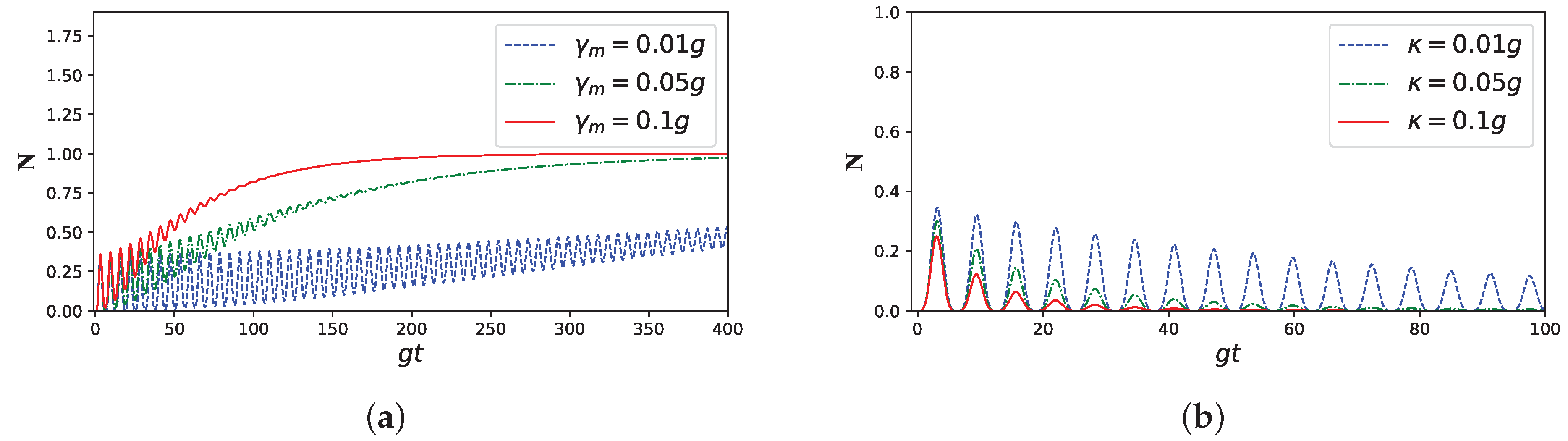
Now, we investigate the time evolution of entanglement under the influence of damping rates (which include atomic, photonic and phononic decay rates) and external pump field amplitude. As you can see in Figure 4, we investigated the effect of atomic and phonon losses on the dynamics of atom–atom entanglement. Regarding Figure 4a, it can be observed that by increasing of the atomic damping rate from to , entanglement oscillates, while its amplitude and its picks are decreased, such that, in a limited time interval, it reaches zero. The number of oscillations is decreased by increasing this decay parameter, in such a way that for , it suddenly decreases from 1 to 0 without any oscillation. Figure 4b is plotted for different values of mirror mechanical loss. As can be seen, some oscillations with decreasing its maximum values are observed. In more detail, the increase in this dissipation parameter leads to the decrease in entanglement. Moreover, in all cases, stability may be achieved, however, in longer times than the previous numerical results. In Figure 5, we aim to investigate the influences of optical field loss and external pump field amplitude on the negativity. In Figure 5a, we can see that by keeping a fixed value for the pump field amplitude, in the presence of field loss rate, again the entanglement oscillates with decreasing its maxima. However, this dissipation parameter has optimal value () in our simulation, for which entanglement stability is achieved sooner (later). But, in Figure 5b, by keeping the photon dissipation rate as a constant , we want to evaluate the effect of external pump field amplitude on the negativity. As is obvious, with the lower value of the pump field, the entanglement stability can be seen. However, with increasing the pump amplitude, fluctuations increase and the stability is gradually destroyed. In particular, in the case of , the entanglement has a more rapid damping behavior such that in the scaled time the negativity dies, but it is revived again and, after some duration of time, again the stable entanglement arrives at the value .
In the following, we want to investigate the atom–atom entanglement with an initial separable state, i.e., its negativity is zero at . We want to check whether or not the stability of entanglement can occur in the presence of optical (Figure 6a) and mechanical (Figure 6b) dissipations for the initial separable state, similar to the initial entangled state (10). It can be seen from Figure 6a that, in this case, the initial state of the system is non-entangled, however, the entanglement increases from zero, its fluctuations decrease with the increase in phonon loss rate, and, after elapsing nearly 150 units of the scaled time, stability has been reached in its maximum possible value, interestingly. While, in Figure 6b, with the increase in the photon loss rate from to , entanglement has been reduced. Moreover, for , a substantial reduction in negativity occurs, and at , entanglement has completely died (entanglement sudden death occurs). In general, it can be observed that with the increase in the phonon loss rate, unlike the photon loss effect, the entanglement reaches its stable value. Finally, it should be noted that the amount of stable entanglement is highly dependent on the phonon damping rate.
4. Summary and Conclusions
In summary, we analyzed an efficient scheme to produce stable bipartite entanglement between two two-level atoms in the absence and under the influences of dissipative effects, with the help of the negativity criterion. In our model, we considered an optomechanical system with linear and quadratic photon–phonon couplings, consisting of a single-mode Fabry–Perot cavity field, which possesses a movable mirror and two two-level atoms exist within it, while the system is driven by two external fields. It is noticeable that, while usually in the literature only the first or the second order of nonlinearity is considered, we did not ignore any of them, as in the very few references [39,51]. After obtaining the interaction Hamiltonian in the interaction picture, the effective Hamiltonian that is independent of time is derived by considering some resonance conditions and the rotating wave approximation. Via the Lindblad master equation, with the effective Hamiltonian of the system, we arrived at the system solution with the existing dissipations arising from atomic, optical and mechanical sources. Then, using the negativity criterion, the entanglement dynamics between the two atoms were analyzed. By considering the appropriate initial states of atoms, the optical field and the mechanical mode, to make it close to experimental reality we have used some laboratory reachable parameters in the typical optomechanical systems [55,56]. Overall, what one may generally conclude from our presented numerical results is that the effect of dissipation parameters is unpredictable and depends highly on the other chosen parameters. In all presented plots, the entanglement oscillates between some maxima and minima, however, among them, there are cases that are more interesting from the point of view of the stability of entanglement. In this regard, we want to emphasize that the atom–atom quasi-stable and even stable entanglement can be observed in the presence of photon as well as phonon dissipation rates. We end this conclusion section by emphasizing that all of the observed entanglement dynamics in this paper, i.e., moderate or high degree, and particularly its stability, are interesting and significant for experimental purposes in different practical protocols in quantum information science and technology platforms.
Author Contributions
Conceptualization, M.R. and M.K.T.; methodology, M.R. and M.K.T.; software, M.R.; validation, M.R. and M.K.T.; formal analysis, M.R. and M.K.T.; investigation, M.R. and M.K.T.; resources, M.R. and M.K.T.; data curation, M.R. and M.K.T.; writing—original draft preparation, M.R.; writing—review and editing, M.K.T.; visualization, M.R. and M.K.T.; supervision, M.K.T.; project administration, Not applicable.; funding acquisition, Not applicable. All authors have read and agreed to the published version of the manuscript.
Funding
No funding exists related to this work.
Data Availability Statement
Not applicable (all data can be found in the article or references therein).
Conflicts of Interest
The authors have no conflict of interest to declare.
References
- Christopher, R.M.; Meekhof, D.M.; King, B.E.; Wineland, D.J. A “Schrödinger Cat” Superposition State of an Atom. Science 1996, 272, 1131. [Google Scholar]
- Nairz, M.A.O.; Andreae, J.V.; Keller, C.; Zouw, G.V.D.; Zeilinger, A. Wave–particle duality of C60 molecules. Nature 1999, 401, 680. [Google Scholar]
- Gerlich, S.; Eibenberger, S.; Tomandl, M.; Nimmrichter, S.; Hornberger, K.; Fagan, P.J.; Tuxen, J.; Mayor, M.; Arndt, M. Quantum interference of large organic molecules. Nat. Commun. 2011, 2, 263. [Google Scholar] [CrossRef] [PubMed]
- Franco, R.L.; Compagno, G. Quantum entanglement of identical particles by standard information-theoretic notions. Sci. Rep. 2016, 6, 20603. [Google Scholar] [CrossRef]
- Pan, J.W.; Gasparoni, S.; Ursin, R.; Weihs, G.; Zeilinger, A. Experimental entanglement purification of arbitrary unknown states. Nature 2003, 423, 417. [Google Scholar] [CrossRef]
- Weedbrook, C.; Pirandola, S.; Patron, R.G.; Cerf, N.J.; Ralph, T.C.; Shapiro, J.H.; Lloyd, S. Gaussian quantum information. Rev. Mod. Phys. 2012, 84, 621. [Google Scholar] [CrossRef]
- Cirac, J.I.; Gisin, N. Coherent eavesdropping strategies for the four state quantum cryptography protocol. Phys. Lett. A 1997, 229, 1–7. [Google Scholar] [CrossRef]
- Fuchs, C.A.; Gisin, N.; Griffiths, R.B.; Niu, C.; Peres, A. Optimal eavesdropping in quantum cryptography. I. Information bound and optimal strategy. Phys. Rev. A 1997, 56, 1163. [Google Scholar] [CrossRef]
- Salimian, S.; Tavassoly, M.K.; Sehati, N. Teleportation of the entangled state of two superconducting qubits. Europhys. Lett. 2021, 138, 55004. [Google Scholar] [CrossRef]
- Li, J.; Wallucks, A.; Benevides, R.; Fiaschi, N.; Hensen, B.; Alegre, T.P.M.; Groblacher, S. Proposal for optomechanical quantum teleportation. Phys. Rev. A 2020, 102, 032402. [Google Scholar] [CrossRef]
- Gyongyosi, L.; Imre, S. A Survey on quantum computing technology. Comput. Sci. Rev. 2019, 31, 51. [Google Scholar] [CrossRef]
- Xu, F.; Ma, X.; Zhang, Q.; Lo, H.K.; Pan, J.W. Secure quantum key distribution with realistic devices. Rev. Mod. Phys. 2020, 92, 025002. [Google Scholar] [CrossRef]
- Liu, Y.; Guo, G.C. Scheme for implementing quantum dense coding in cavity QED. Phys. Rev. A 2005, 71, 034304. [Google Scholar]
- Mozes, S.; Reznik, B.; Oppenheim, J. Deterministic dense coding with partially entangled states. Phys. Rev. A 2005, 71, 012311. [Google Scholar] [CrossRef]
- Kwiat, P.G.; Mattle, K.; Weinfurter, H.; Zeilinger, A.; Sergienko, A.; Shih, Y. New high-intensity source of polarization-entangled photon pairs. Phys. Lett. A 1995, 75, 4337. [Google Scholar] [CrossRef]
- Hagley, E.W.; Maitre, X.; Nogues, G.; Wunderlich, C.; Brune, M.; Raimond, J.M.; Haroche, S. Generation of Einstein-Podolsky-Rosen Pairs of Atoms. Phys. Rev. Lett. 1997, 79, 1. [Google Scholar] [CrossRef]
- Turchette, Q.A.; Wood, C.S.; King, B.E.; Myatt, C.J.; Leibfried, D.; Itano, W.M.; Monroe, C.R.; Wineland, D.J. Deterministic Entanglement of Two Trapped Ions. Phys. Rev. Lett. 1998, 81, 3631. [Google Scholar] [CrossRef]
- Rafeie, M.; Tavassoly, M.K.; Kheirabady, M.S. Macroscopic Mechanical Entanglement Stability in Two Distant Dissipative Optomechanical Systems. Ann. Phys. 2022, 534, 2100455. [Google Scholar] [CrossRef]
- Wu, Q.; Ma, P.C. Tunable double optomechanical induced transparency in an optomechanical system with Bose–Einstein condensate. J. Mod. Opt. 2017, 64, 685. [Google Scholar] [CrossRef]
- Yi, C.Q.; Yi, Z.; Gu, W.J.; Xu, D.H. Generating EPR-type entanglement of degenerate optomechanical parametric oscillators. J. Mod. Opt. 2017, 64, 2103. [Google Scholar] [CrossRef]
- Kong, C.; Li, S.; You, C.; Xiong, H.; Wu, Y. Two-color second-order sideband generation in an optomechanical system with a two-level system. Sci. Rep. 2018, 8, 1060. [Google Scholar] [CrossRef] [PubMed]
- Nadiki, M.H.; Tavassoly, M.K. The amplitude of the cavity pump field and dissipation effects on the entanglement dynamics and statistical properties of an optomechanical system. Opt. Commun. 2019, 452, 31. [Google Scholar] [CrossRef]
- Wang, K.; Gao, Y.P.; Jiao, R.; Wang, C. Recent progress on optomagnetic coupling and optical manipulation based on cavity-optomagnonics. Front. Phys. 2022, 17, 42201. [Google Scholar] [CrossRef]
- Ghasemi, M.; Tavassoly, M.K.; Nourmandipour, A. Dissipative entanglement swapping in the presence of detuning and Kerr medium: Bell state measurement method. Eur. Phys. J. Plus 2017, 132, 531. [Google Scholar] [CrossRef]
- Liu, N.; Li, J.Q.; Liang, J.Q. Entanglement in a Tripartite Cavity-Optomechanical System. Int. J. Theor. Phys. 2013, 52, 706. [Google Scholar] [CrossRef]
- Kippenberg, J.T.; Vahala, K.J. Cavity optomechanics: Back-action at the mesoscale. Science 2008, 321, 1172. [Google Scholar] [CrossRef] [PubMed]
- Aspelmeyer, M.; Meystre, P.; Schwab, K. Quantum optomechanics. Phys. Today 2012, 65, 29. [Google Scholar] [CrossRef]
- Aspelmeyer, M.; Kippenberg, T.J.; Marquardt, F. Cavity optomechanics. Rev. Mod. Phys. 2014, 86, 1391. [Google Scholar] [CrossRef]
- Gao, Y.P.; Cao, C.; Lu, P.F.; Wang, C. Phase-controlled photon blockade in optomechanical systems. Fundam. Res. 2023, 3, 30. [Google Scholar] [CrossRef]
- Yu, Y.; Liu, H.Y. Photon antibunching in unconventional photon blockade with Kerr nonlinearities. J. Mod. Opt. 2017, 64, 1342. [Google Scholar] [CrossRef]
- Zhai, C.; Huang, R.; Jing, H.; Kuang, L.M. Mechanical switch of photon blockade and photon-induced tunneling. Opt. Express 2019, 27, 27649. [Google Scholar] [CrossRef]
- Yang, J.Y.; Jin, Z.; Liu, J.S.; Wang, H.F.; Zhu, A.D. Unconventional Phonon Blockade in a Tavis-Cummings Coupled Optomechanical System. Ann. Phys. 2020, 532, 2000299. [Google Scholar] [CrossRef]
- Wang, M.; Lu, X.Y.; Miranowicz, A.; Yi, T.S.; Wu, Y.; Nori, F. Unconventional phonon blockade via atom-photon-phonon interaction in hybrid optomechanical systems. Opt. Express 2022, 30, 10251. [Google Scholar] [CrossRef] [PubMed]
- Tan, H.T.; Li, G.X.; Meystre, P. Dissipation-driven two-mode mechanical squeezed states in optomechanical systems. Phys. Rev. A 2013, 87, 033829. [Google Scholar] [CrossRef]
- Sainadh, U.S.; Kumar, M.A. Squeezing of the mechanical motion and beating 3 dB limit using dispersive optomechanical interactions. J. Mod. Opt. 2016, 64, 1121. [Google Scholar] [CrossRef]
- Huang, S.; Chen, A. Mechanical squeezing in a dissipative optomechanical system with two driving tones. Phys. Rev. A 2021, 103, 023501. [Google Scholar] [CrossRef]
- Nunnenkamp, A.; Borkje, K.; Harris, J.G.E.; Girvin, S.M. Cooling and squeezing via quadratic optomechanical coupling. Phys. Rev. A 2010, 82, 021806. [Google Scholar] [CrossRef]
- SatyaSainadh, U.; Kumar, M.A. Effects of linear and quadratic dispersive couplings on optical squeezing in an optomechanical system. Phys. Rev. A 2015, 92, 033824. [Google Scholar]
- Gu, W.J.; Yi, Z.; Yan, Y.; Sun, L.H. Generation of Optical and Mechanical Squeezing in the Linear-and-Quadratic Optomechanics. Ann. Phys. 2019, 531, 1800399. [Google Scholar] [CrossRef]
- Liao, J.Q.; Nori, F. Photon blockade in quadratically coupled optomechanical systems. Phys. Rev. A 2013, 88, 023853. [Google Scholar] [CrossRef]
- Wan, K.; Gao, Y.P.; Pang, T.T.; Wang, T.; Wang, C. Enhanced photon blockade in quadratically coupled optomechanical system. EPL 2020, 131, 24003. [Google Scholar]
- Zhang, J.S.; Li, M.C.; Chen, A.X. Enhancing quadratic optomechanical coupling via a nonlinear medium and lasers. Phys. Rev. A 2019, 99, 013843. [Google Scholar] [CrossRef]
- Rabl, P. Photon blockade effect in optomechanical systems. Phys. Rev. Lett. 2011, 107, 063601. [Google Scholar] [CrossRef] [PubMed]
- Nunnenkamp, A.; Borkje, K.; Girvin, S.M. Single-photon optomechanics. Phys. Rev. Lett. 2011, 107, 063602. [Google Scholar] [CrossRef]
- Li, Z.Y.; Jin, G.R.; Yin, T.S.; Chen, A. Two-Phonon Blockade in Quadratically Coupled Optomechanical Systems. Photonics 2022, 9, 70. [Google Scholar] [CrossRef]
- Nadiki, M.H.; Tavassoly, M.K. Phonon blockade in a system consisting of two optomechanical cavities with quadratic cavity-membrane coupling and phonon hopping. Eur. Phys. J. Plus D 2022, 76, 58. [Google Scholar] [CrossRef]
- Xie, H.Y.; Liao, C.G.; Shang, X.; Ye, M.Y.; Lin, X. Phonon blockade in a quadratically coupled optomechanical system. Phys. Rev. A 2017, 96, 013861. [Google Scholar] [CrossRef]
- Zheng, L.L.; Yin, T.S.; Bin, Q.; Lu, X.U.; Wu, Y. Single-photon-induced phonon blockade in a hybrid spin-optomechanical system. Phys. Rev. A 2019, 99, 013804. [Google Scholar] [CrossRef]
- Rafeie, M.; Tavassoly, M.K. Quantum statistics and blockade of phonon and photon in a dissipative quadratically coupled optomechanical system. Eur. Phys. J. D 2023, 77, 63. [Google Scholar] [CrossRef]
- Vitali, D.; Gigan, S.; Ferreira, A.; Böhm, H.R.; Tombesi, P.; Guerreiro, A.; Vedral, V.; Zeilinger, A.; Aspelmeyer, M. Optomechanical entanglement between a movable mirror and a cavity field. Phys. Rev. Lett. 2007, 98, 030405. [Google Scholar] [CrossRef]
- Zhang, X.Y.; Zhou, Y.H.; Guo, Y.Q.; Yi, X.X. Optomechanically induced transparency in optomechanics with both linear and quadratic coupling. Phys. Rev. A 2018, 98, 053802. [Google Scholar] [CrossRef]
- James, D.F.V.; Jerke, J. Effective Hamiltonian theory and its applications in quantum information. Can. J. Phys. 2007, 85, 625. [Google Scholar] [CrossRef]
- Carmichael, H.J. Statistical Methods in Quantum Optics 1; Springer: Berlin, Germany, 1999. [Google Scholar]
- Vidal, G.; Werner, R.F. Computable measure of entanglement. Phys. Rev. A 2002, 65, 032314. [Google Scholar] [CrossRef]
- Hood, C.J.; Lynn, T.; Mabuchi, H.; Chapman, M.S.; Ye, J.; Kimble, H.J. Real-time cavity QED with single atoms. Phys. Rev. Lett. 1998, 80, 6. [Google Scholar] [CrossRef]
- Bose, S.; Jacobs, K.; Knight, P.L. A Quantum Optical Scheme to Probe the Decoherence of a Macroscopic Object. Phys. Rev. A 1999, 59, 3204. [Google Scholar] [CrossRef]
- Thompson, J.D.; Zwickl, B.M.; Jayich, A.M.; Marquardt, F.; Girvin, S.M.; Harris, J.G.E. Strong dispersive coupling of a high-finesse cavity to a micromechanical membrane. Nature 2008, 452, 72. [Google Scholar] [CrossRef] [PubMed]
- Sankey, J.C.; Yang, C.; Zwickl, B.M.; Jayich, A.M.; Harris, J.G.E. Strong and tunable nonlinear optomechanical coupling in a low-loss system. Nature 2010, 6, 707. [Google Scholar] [CrossRef]
- NJacobs, E.F.; Hoch, S.W.; Sankey, J.; Kashkanova, A.; Jayich, A.M.; Deutsch, C.; Reichel, J.; Harris, J.G.E. Fiber-cavity-based optomechanical device. Appl. Phys. Lett. 2012, 101, 221109. [Google Scholar]
- Li, H.; Liu, Y.C.; Yi, X.; Zou, C.L.; Ren, X.; Xiao, Y.F. Proposal for a near-field optomechanical system with enhanced linear and quadratic coupling. Phys. Rev. A 2012, 85, 053832. [Google Scholar] [CrossRef]
Figure 1.
Schematic structure of the considered system. An optomechanical cavity is driven by an external pump field with frequency and amplitude . Two two-level atoms exist in the cavity, which interact with the classical as well as the quantized field. The frequency and the amplitude of the classical field read as and , respectively. The parameters , and refer to atomic, mirror and cavity dissipation rates, respectively.

Figure 2.
Negativity as a function of the scaled time for different coherent angles, i.e., (a), (b), (c). Other parameters in (a–c) are chosen as .
Figure 2.
Negativity as a function of the scaled time for different coherent angles, i.e., (a), (b), (c). Other parameters in (a–c) are chosen as .
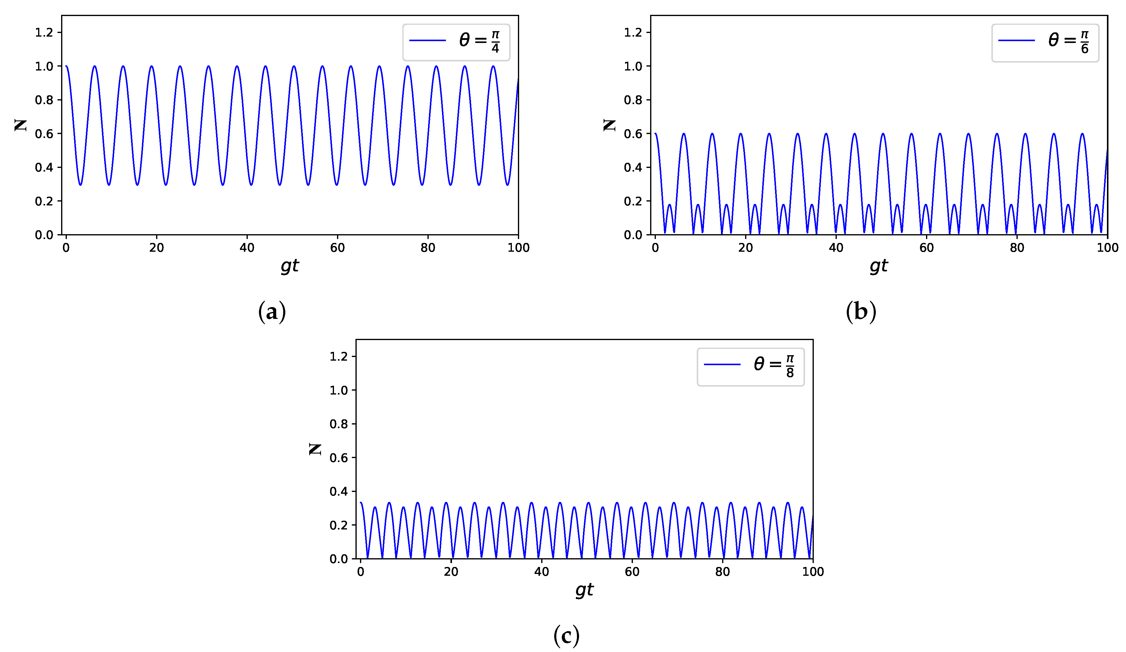
Figure 3.
Negativity as a function of the scaled time for different values of nonlinear optomechanical term, i.e., (a), (b), (c). Other parameters in (a–c) are chosen as Figure 2, except that .
Figure 3.
Negativity as a function of the scaled time for different values of nonlinear optomechanical term, i.e., (a), (b), (c). Other parameters in (a–c) are chosen as Figure 2, except that .
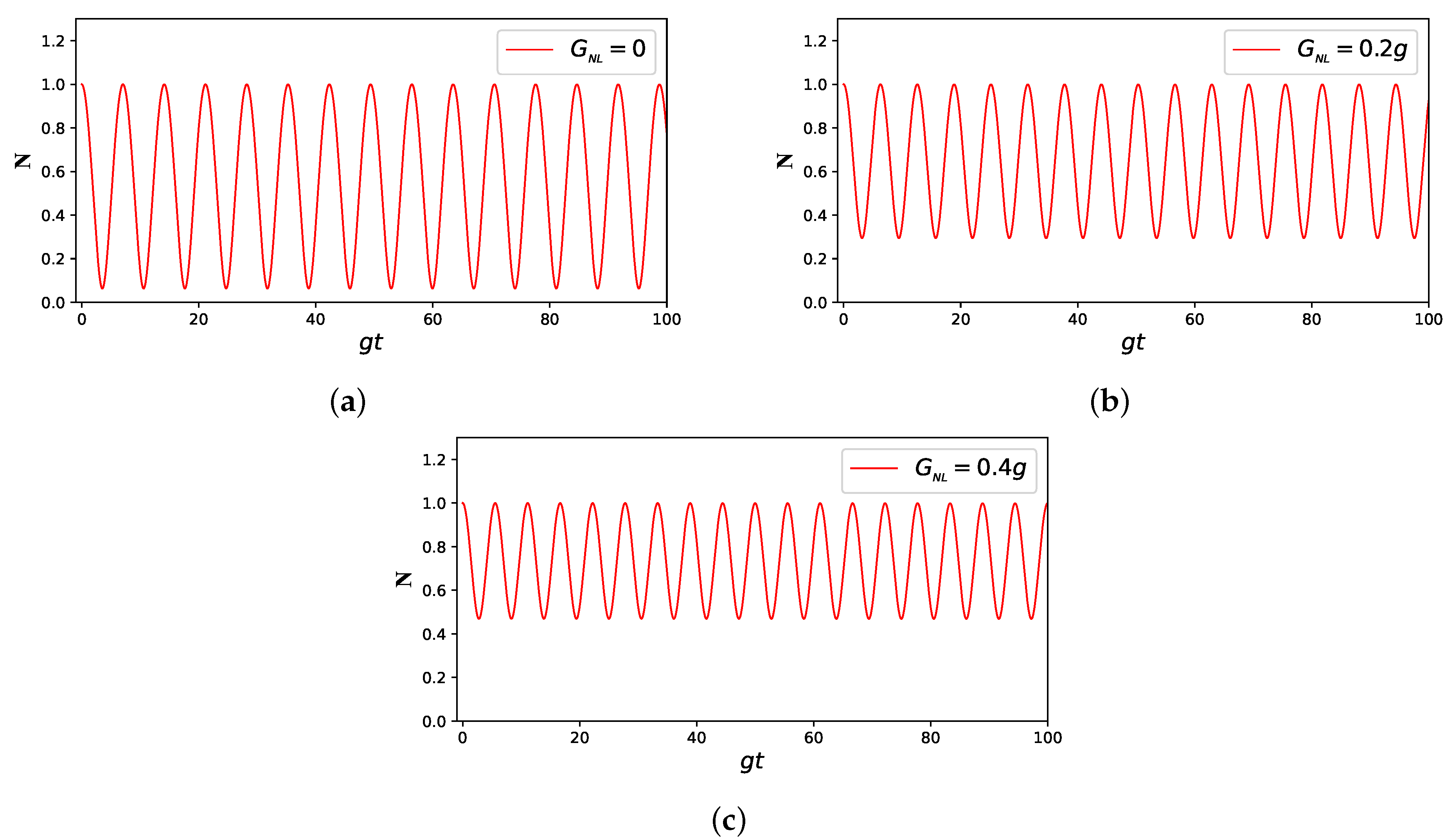
Figure 4.
Negativity as a function of the scaled time for different values of atomic (a) and phononic (b) decay rates. The chosen parameters are as in Figure 2, except that and in (a) and in (b) .
Figure 4.
Negativity as a function of the scaled time for different values of atomic (a) and phononic (b) decay rates. The chosen parameters are as in Figure 2, except that and in (a) and in (b) .

Figure 5.
Negativity as a function of the scaled time for different values of photonic decay rates (a) and pump field amplitudes (b). The chosen parameters are as Figure 2, except that .
Figure 5.
Negativity as a function of the scaled time for different values of photonic decay rates (a) and pump field amplitudes (b). The chosen parameters are as Figure 2, except that .

Figure 6.
Negativity as a function of the scaled time for different values of phononic (a) and photonic (b) decay rates. The chosen parameters are as Figure 2, except that and in (a) and in (b) .
Figure 6.
Negativity as a function of the scaled time for different values of phononic (a) and photonic (b) decay rates. The chosen parameters are as Figure 2, except that and in (a) and in (b) .
Disclaimer/Publisher’s Note: The statements, opinions and data contained in all publications are solely those of the individual author(s) and contributor(s) and not of MDPI and/or the editor(s). MDPI and/or the editor(s) disclaim responsibility for any injury to people or property resulting from any ideas, methods, instructions or products referred to in the content. |
© 2023 by the authors. Licensee MDPI, Basel, Switzerland. This article is an open access article distributed under the terms and conditions of the Creative Commons Attribution (CC BY) license (https://creativecommons.org/licenses/by/4.0/).
Share and Cite
MDPI and ACS Style
Rafeie, M.; Tavassoly, M.K. Generation of Stable Entanglement in an Optomechanical System with Dissipative Environment: Linear-and-Quadratic Couplings. Symmetry 2023, 15, 1770. https://doi.org/10.3390/sym15091770
AMA Style
Rafeie M, Tavassoly MK. Generation of Stable Entanglement in an Optomechanical System with Dissipative Environment: Linear-and-Quadratic Couplings. Symmetry. 2023; 15(9):1770. https://doi.org/10.3390/sym15091770
Chicago/Turabian StyleRafeie, Mehran, and Mohammad Kazem Tavassoly. 2023. "Generation of Stable Entanglement in an Optomechanical System with Dissipative Environment: Linear-and-Quadratic Couplings" Symmetry 15, no. 9: 1770. https://doi.org/10.3390/sym15091770
Note that from the first issue of 2016, this journal uses article numbers instead of page numbers. See further details here.