
A Proposed DEA Window Analysis for Assessing Efficiency from Asymmetry Dynamic Data


Abstract
:1. Introduction
2. Literature Review
3. Research Methodology
4. Research Results
5. Conclusions
Author Contributions
Funding
Data Availability Statement
Conflicts of Interest
References
- Kumar, S.; Gulati, R. An examination of technical, pure technical, and scale efficiencies in Indian public sector banks using data envelopment analysis. Eurasian J. Bus. Econ. 2008, 1, 33–69. [Google Scholar]
- Al-Refaie, A. Window Analysis and MPI for Efficiency and Productivity Assessment Under Fuzzy Data: Window Analysis and MPI. Int. J. Manuf. Mater. Mech. Eng. 2022, 12, 22. [Google Scholar] [CrossRef]
- Al-Refaie, A.; Ghaleb Abbasi, G.; Al-Hawadi, A. DEA Efficiency Assessment of Packaging Lines in A Pharmaceutical Industry. Eng. Lett. 2023, 31, 1241–1249. [Google Scholar]
- Davutyan, N.; Yildirim, C. Efficiency in Turkish banking: Post-restructuring evidence. Eur. J. Financ. 2017, 23, 170–191. [Google Scholar] [CrossRef]
- Ennen, D.; Batool, I. Airport efficiency in Pakistan-A Data Envelopment Analysis with weight restrictions. J. Air Transp. Manag. 2018, 69, 205–212. [Google Scholar] [CrossRef]
- Al-Refaie, A.; Hammad, M.; Li, M.H. DEA window analysis and Malmquist index to assess energy efficiency and productivity in Jordanian industrial sector. Energy Effic. 2016, 9, 1299–1313. [Google Scholar] [CrossRef]
- Charnes, A.; Cooper, W.W.; Rhodes, E. Measuring the Efficiency of Decision Making Units. Eur. J. Oper. Res. 1978, 2, 429–444. [Google Scholar] [CrossRef]
- Cooper, W.W.; Seiford, L.M.; Tone, K. Introduction to Data Envelopment Analysis and Its Uses: With DEA-Solver Software and References; Springer Science & Business Media: Berlin/Heidelberg, Germany, 2006. [Google Scholar]
- Cooper, W.W.; Seiford, L.M.; Zhu, J. Data envelopment analysis: History, models, and interpretations. In Handbook on Data Envelopment Analysis; Springer: Boston, MA, USA, 2011; pp. 1–39. [Google Scholar]
- Ma, J.; Evans, D.G.; Fuller, R.J.; Stewart, D.F. Technical efficiency and productivity change of China’s iron and steel industry. Int. J. Prod. Econ. 2002, 76, 293–312. [Google Scholar] [CrossRef]
- Chen, C.J.; Wu, H.L.; Lin, B.W. Evaluating the development of high-tech industries: Taiwan’s science park. Technol. Forecast. Soc. Chang. 2006, 73, 452–465. [Google Scholar] [CrossRef]
- Barros, C.P.; Dieke, P.U. Performance evaluation of Italian airports: A data envelopment analysis. J. Air Transp. Manag. 2007, 13, 184–191. [Google Scholar] [CrossRef]
- Barros, C.P.; Dieke, P.U. Technical efficiency of African hotels. Int. J. Hosp. Manag. 2008, 27, 438–447. [Google Scholar] [CrossRef]
- Keskin, B.Y.; Degirmen, S. The application of data envelopment analysis based Malmquist total factor productivity index: Empirical evidence in Turkish banking sector. Panoeconomicus 2013, 60, 139–159. [Google Scholar] [CrossRef]
- Balcerzak, A.P.; Kliestik, T.; Streimikiene, D.; Smrcka, L. Non-parametric approach to measuring the efficiency of banking sectors in European Union Countries. Acta Polytech. Hung. 2017, 14, 51–70. [Google Scholar]
- Yang, H.H.; Chang, C.Y. Using DEA window analysis to measure efficiencies of Taiwan’s integrated telecommunication firms. Telecommun. Policy 2009, 33, 98–108. [Google Scholar] [CrossRef]
- Diskaya, F.; Emir, S.; Orhan, N. Measuring the technical efficiency of telecommunication sector within global crisis: Comparison of G8 countries and Turkey. Procedia Soc. Behav. Sci. 2011, 24, 206–218. [Google Scholar] [CrossRef]
- Pulina, M.; Detotto, C.; Paba, A. An investigation into the relationship between size and efficiency of the Italian hospitality sector: A window DEA approach. Eur. J. Oper. Res. 2010, 204, 613–620. [Google Scholar] [CrossRef]
- Mahajan, V.; Nauriyal, D.K.; Singh, S.P. Technical efficiency analysis of the Indian drug and pharmaceutical industry: A non-parametric approach. Benchmarking Int. J. 2014, 21, 734–755. [Google Scholar] [CrossRef]
- Jia, T.; Yuan, H. The application of DEA (Data Envelopment Analysis) window analysis in the assessment of influence on operational efficiencies after the establishment of branched hospitals. BMC Health Serv. Res. 2017, 17, 265. [Google Scholar] [CrossRef]
- Al-Refaie, A.; Al-Tahat, M.D.; Najdawi, R. Using Malmquist index approach to measure productivity change of a Jordanian company for plastic industries. Am. J. Oper. Res. 2015, 5, 384. [Google Scholar] [CrossRef]
- Al-Refaie, A.; Wu, C.W.; Sawalheh, M. DEA window analysis for assessing efficiency of blistering process in a pharmaceutical industry. Neural Comput. Appl. 2019, 31, 3703–3717. [Google Scholar] [CrossRef]
- Peykani, P.; Mohammadi, E. Window network data envelopment analysis: An application to investment companies. Int. J. Ind. Math. 2020, 12, 89–99. [Google Scholar]
- Seth, S.; Feng, Q. Assessment of port efficiency using stepwise selection and window analysis in data envelopment analysis. Marit. Econ. Logist. 2020, 22, 536–561. [Google Scholar] [CrossRef]
- Akhtar, S.; Alam, M.; Ansari, M.S. Measuring the performance of the Indian banking industry: Data envelopment window analysis approach. Benchmarking Int. J. 2021, 29, 2842–2857. [Google Scholar] [CrossRef]
- Guo, P.; Tanaka, H. Fuzzy DEA: A perceptual evaluation method. Fuzzy Sets Syst. 2001, 119, 149–160. [Google Scholar] [CrossRef]
- Lertworasirikul, S.; Fang, S.C.; Joines, J.A.; Nuttle, H.L. Fuzzy data envelopment analysis (DEA): A possibility approach. Fuzzy Sets Syst. 2003, 139, 379–394. [Google Scholar] [CrossRef]
- Liu, S.T.; Chuang, M. Fuzzy efficiency measures in fuzzy DEA/AR with application to university libraries. Expert Syst. Appl. 2009, 36, 1105–1113. [Google Scholar] [CrossRef]
- Wen, M.; Li, H. Fuzzy data envelopment analysis (DEA): Model and ranking method. J. Comput. Appl. Math. 2009, 223, 872–878. [Google Scholar] [CrossRef]
- Puri, J.; Yadav, S.P. A concept of fuzzy input mix-efficiency in fuzzy DEA and its application in banking sector. Expert Syst. Appl. 2013, 40, 1437–1450. [Google Scholar] [CrossRef]
- Wanke, P.; Barros, C.P.; Nwaogbe, O.R. Assessing productive efficiency in Nigerian airports using Fuzzy-DEA. Transp. Policy 2016, 49, 9–19. [Google Scholar] [CrossRef]
- Barak, S.; Dahooei, J.H. A novel hybrid fuzzy DEA-Fuzzy MADM method for airlines safety evaluation. J. Air Transp. Manag. 2018, 73, 134–149. [Google Scholar] [CrossRef]
- Arana-Jiménez, M.; Sánchez-Gil, M.C.; Lozano, S. A fuzzy DEA slacks-based approach. J. Comput. Appl. Math. 2022, 404, 113180. [Google Scholar] [CrossRef]
- Khoshandam, L.; Nematizadeh, M. An inverse network DEA model for two-stage processes in the presence of undesirable factors. J. Appl. Res. Ind. Eng. 2023, 10, 155–166. [Google Scholar] [CrossRef]
- Mohanta, K.K.; Sharanappa, D.S.; Edalatpanah, S.A. A Novel Technique for Solving Intuitionistic Fuzzy DEA Model: An Application in Indian Agriculture Sector. Res. Sq. 2023. [Google Scholar] [CrossRef]
- Wang, C.N.; Dang, T.T.; Tibo, H.; Duong, D.H. Assessing renewable energy production capabilities using DEA window and fuzzy TOPSIS model. Symmetry 2021, 13, 334. [Google Scholar] [CrossRef]
- Peykani, P.; Memar-Masjed, E.; Arabjazi, N.; Mirmozaffari, M. Dynamic performance assessment of hospitals by applying credibility-based fuzzy window data envelopment analysis. Healthcare 2022, 10, 876. [Google Scholar] [CrossRef]
- Jamshidi, A.; Yazdani-Chamzini, A.; Yakhchali, S.H.; Khaleghi, S. Developing a new fuzzy inference system for pipeline risk assessment. J. Loss Prev. Process Ind. 2013, 26, 197–208. [Google Scholar] [CrossRef]
- Nepomuceno, T.C.C. Data-driven Analytics for Socioeconomic Challenges in a Contemporary World. Socioecon. Anal. 2023, 1, 1–4. [Google Scholar]
- Salari, M.; Khamooshi, H. A better project performance prediction model using fuzzy time series and data envelopment analysis. J. Oper. Res. Soc. 2016, 67, 1274–1287. [Google Scholar] [CrossRef]


| Inputs/Outputs of DMU1 (k = 1) | t = 1 | … | t = 6 |
|---|---|---|---|
| … | |||
| … | |||
| ⋮ | ⋮ | ⋮ | |
| … | |||
| … | |||
| … | |||
| ⋮ | ⋮ | ⋮ | |
| … |
| Inputs/Outputs of DMU1 (k = 1) at Low-Level Data | t = 1 | … | t = 6 | ||
|---|---|---|---|---|---|
| ait1 | a111 | … | a161 | ||
| a211 | … | a261 | |||
| ⋮ | ⋮ | ⋮ | |||
| am11 | … | am61 | |||
| drt1 | d111 | … | d161 | ||
| d211 | … | d261 | |||
| ⋮ | ⋮ | ⋮ | |||
| ds11 | … | ds61 | |||
| Averages of optimal TE and PTE at low-level data | |||||
| DMUj | t = 1 | t = 2 | … | t = 6 | t = 7 | t = 11 | t = 12 | DMU Efficiency | |
|---|---|---|---|---|---|---|---|---|---|
| DMU1 | … | ||||||||
| DMU2 | … | ||||||||
| ⋮ | ⋮ | ⋮ | ⋮ | ||||||
| DMU6 | … | ||||||||
| DMU7 | … | ||||||||
| Period efficiency |
| Period t | Inputs | Output | ||
|---|---|---|---|---|
| Planned Production | Defectives | Idle Time | Production Quantity | |
| 1 | (24150, 24192, 25100) | (179, 185, 192) | (1383,1426, 1483) | (21099, 22300, 23103) |
| 2 | (24100, 24192, 24300) | (91, 94, 97) | (7756, 7996, 8315) | (15550, 15731, 17832) |
| 3 | (24000, 24192, 25159) | (66, 69, 71) | (3054, 3149, 3274) | (20549, 21419, 22318) |
| 4 | (24000, 24192, 25000) | (94, 97, 100) | (6221, 6414, 6670) | (18231, 18359, 23721) |
| 5 | (20113, 20736,21565) | (170, 176, 183) | (1876, 1935, 2012) | (17128, 17221, 19762) |
| 6 | (26818, 27648, 28753) | (137, 142, 147) | (49, 51, 53) | (26810, 27620, 27640) |
| 7 | (23466, 24192, 25159) | (116, 120, 124) | (3317, 3420, 3556) | (18089, 19456, 22941) |
| 8 | (20113, 20736, 21565) | (51, 53, 55) | (2018, 2081, 2164) | (19012, 19616, 20000) |
| 9 | (13409, 13824, 14376) | (31, 32, 33) | (657, 678, 705) | (12984, 13500, 13561) |
| 10 | (10056, 10368, 10782) | (70, 73, 75) | (2769, 2855, 2969) | (8195, 8318, 9939) |
| 11 | (15085, 15552, 16174) | (111, 115, 119) | (2873, 2962, 3080) | (13294, 13350, 15230) |
| 12 | (21790, 22464, 23362) | (237, 245, 254) | (2268, 2339, 2432) | (20137, 20750, 22252) |
| DMU | Period t | |||||||||||||
|---|---|---|---|---|---|---|---|---|---|---|---|---|---|---|
| j | 1 | 2 | 3 | 4 | 5 | 6 | 7 | 8 | 9 | 10 | 11 | 12 | CV% | |
| 1 | 0.8739 | 0.7024 | 1.0000 | 0.8193 | 0.8518 | 1.0000 | 0.8746 | 13.01% | ||||||
| 2 | 0.7024 | 1.0000 | 0.8193 | 0.8518 | 1.0000 | 0.7789 | 0.8587 | 14.01% | ||||||
| 3 | 0.9015 | 0.7795 | 0.8518 | 1.0000 | 0.7738 | 1.0000 | 0.8844 | 11.45% | ||||||
| 4 | 0.7702 | 0.8518 | 1.0000 | 0.7725 | 0.9737 | 1.0000 | 0.8947 | 12.31% | ||||||
| 5 | 0.8518 | 1.0000 | 0.7725 | 0.9737 | 1.0000 | 0.8152 | 0.9022 | 11.21% | ||||||
| 6 | 1.0000 | 0.7725 | 0.9737 | 1.0000 | 0.8152 | 0.8815 | 0.9072 | 10.90% | ||||||
| 7 | 0.7961 | 0.9762 | 1.0000 | 0.8416 | 0.9101 | 0.9544 | 0.9131 | 8.77% | ||||||
| 0.8739 | 0.7024 | 0.9672 | 0.7971 | 0.8518 | 1.0000 | 0.7777 | 0.9795 | 1.0000 | 0.8240 | 0.8958 | 0.9544 | |||
| CV% | 0.00% | 0.00% | 5.88% | 3.25% | 0.00% | 0.00% | 1.20% | 1.18% | 0.00% | 1.85% | 2.26% | 0.00% | ||
| j | 1 | 2 | 3 | 4 | 5 | 6 | 7 | 8 | 9 | 10 | 11 | 12 | CV% | |
| 1 | 0.9227 | 0.6941 | 1.0000 | 0.8048 | 0.8313 | 1.0000 | 0.8755 | 13.81% | ||||||
| 2 | 0.6941 | 1.0000 | 0.8048 | 0.8313 | 1.0000 | 0.8122 | 0.8571 | 14.08% | ||||||
| 3 | 0.9299 | 0.7777 | 0.8313 | 1.0000 | 0.8080 | 1.0000 | 0.8912 | 11.06% | ||||||
| 4 | 0.7665 | 0.8313 | 1.0000 | 0.8062 | 0.9668 | 1.0000 | 0.8951 | 11.79% | ||||||
| 5 | 0.8313 | 1.0000 | 0.8062 | 0.9668 | 1.0000 | 0.8031 | 0.9012 | 10.80% | ||||||
| 6 | 1.0000 | 0.8062 | 0.9668 | 1.0000 | 0.8031 | 0.8593 | 0.9059 | 10.37% | ||||||
| 7 | 0.8235 | 0.9687 | 1.0000 | 0.8215 | 0.8790 | 0.9459 | 0.9064 | 8.41% | ||||||
| 0.9227 | 0.6941 | 0.9766 | 0.7885 | 0.8313 | 1.0000 | 0.8104 | 0.9738 | 1.0000 | 0.8092 | 0.8692 | 0.9459 | |||
| CV% | 0.00% | 0.00% | 4.14% | 2.46% | 0.00% | 0.00% | 0.84% | 1.51% | 0.00% | 1.31% | 1.60% | 0.00% | ||
| j | 1 | 2 | 3 | 4 | 5 | 6 | 7 | 8 | 9 | 10 | 11 | 12 | CV% | |
| 1 | 0.9575 | 0.7737 | 1.0000 | 1.0000 | 0.9533 | 1.0000 | 0.9474 | 9.28% | ||||||
| 2 | 0.7737 | 1.0000 | 1.0000 | 0.9533 | 1.0000 | 0.9506 | 0.9463 | 9.27% | ||||||
| 3 | 0.9524 | 1.0000 | 0.9533 | 1.0000 | 0.9506 | 1.0000 | 0.9761 | 2.69% | ||||||
| 4 | 0.9944 | 0.9533 | 1.0000 | 0.9497 | 0.9815 | 1.0000 | 0.9798 | 2.35% | ||||||
| 5 | 0.9533 | 1.0000 | 0.9497 | 0.9815 | 1.0000 | 0.9589 | 0.9739 | 2.37% | ||||||
| 6 | 1.0000 | 0.9497 | 0.9815 | 1.0000 | 0.9589 | 0.9796 | 0.9783 | 2.12% | ||||||
| 7 | 0.9638 | 0.9829 | 1.0000 | 0.9721 | 0.9925 | 1.0000 | 0.9852 | 1.52% | ||||||
| 0.9575 | 0.7737 | 0.9841 | 0.9986 | 0.9533 | 1.0000 | 0.9524 | 0.9855 | 1.0000 | 0.9633 | 0.9861 | 1.0000 | |||
| CV% | 0.00% | 0.00% | 2.79% | 0.28% | 0.00% | 0.00% | 0.59% | 0.83% | 0.00% | 0.79% | 0.93% | 0.00% | ||
| Period t | ||||||||||||||
|---|---|---|---|---|---|---|---|---|---|---|---|---|---|---|
| DMUj | 1 | 2 | 3 | 4 | 5 | 6 | 7 | 8 | 9 | 10 | 11 | 12 | CV% | |
| 1 | 0.9467 | 0.9624 | 1.0000 | 0.9620 | 1.0000 | 1.0000 | 0.9785 | 2.47% | ||||||
| 2 | 0.9624 | 1.0000 | 0.9620 | 1.0000 | 1.0000 | 0.9520 | 0.9794 | 2.34% | ||||||
| 3 | 1.0000 | 0.8380 | 1.0000 | 1.0000 | 0.8571 | 1.0000 | 0.9492 | 8.32% | ||||||
| 4 | 0.7707 | 0.8665 | 1.0000 | 0.7824 | 1.0000 | 1.0000 | 0.9033 | 12.29% | ||||||
| 5 | 0.8665 | 1.0000 | 0.7824 | 1.0000 | 1.0000 | 1.0000 | 0.9415 | 10.03% | ||||||
| 6 | 1.0000 | 0.7824 | 1.0000 | 1.0000 | 1.0000 | 0.9088 | 0.9485 | 9.40% | ||||||
| 7 | 0.8134 | 1.0000 | 1.0000 | 1.0000 | 0.9118 | 1.0000 | 0.9542 | 8.12% | ||||||
| 0.9467 | 0.9624 | 1.0000 | 0.8832 | 0.9466 | 1.0000 | 0.8283 | 1.0000 | 1.0000 | 1.0000 | 0.9103 | 1.0000 | |||
| CV% | 0 | 0.00% | 0.00% | 10.77% | 7.72% | 0.00% | 8.13% | 0.00% | 0.00% | 0.00% | 0.23% | 0.00% | ||
| DMUj | 1 | 2 | 3 | 4 | 5 | 6 | 7 | 8 | 9 | 10 | 11 | 12 | CV% | |
| 1 | 0.9967 | 0.9703 | 1.0000 | 0.9669 | 1.0000 | 1.0000 | 0.9890 | 1.61% | ||||||
| 2 | 0.9703 | 1.0000 | 0.9669 | 1.0000 | 1.0000 | 0.9413 | 0.9798 | 2.48% | ||||||
| 3 | 1.0000 | 0.8571 | 1.0000 | 1.0000 | 0.8571 | 1.0000 | 0.9524 | 7.75% | ||||||
| 4 | 0.7681 | 0.8424 | 1.0000 | 0.8125 | 1.0000 | 1.0000 | 0.9038 | 11.95% | ||||||
| 5 | 0.8424 | 1.0000 | 0.8125 | 1.0000 | 1.0000 | 1.0000 | 0.9425 | 9.51% | ||||||
| 6 | 1.0000 | 0.8125 | 1.0000 | 1.0000 | 1.0000 | 0.8825 | 0.9492 | 8.62% | ||||||
| 7 | 0.8497 | 1.0000 | 1.0000 | 1.0000 | 0.8825 | 1.0000 | 0.9554 | 7.32% | ||||||
| 0.9967 | 0.9703 | 1.0000 | 0.8898 | 0.9370 | 1.0000 | 0.8476 | 1.0000 | 1.0000 | 1.0000 | 0.8825 | 1.0000 | |||
| CV% | 0 | 0.00% | 0.00% | 10.81% | 9.21% | 0.00% | 5.92% | 0.00% | 0.00% | 0.00% | 0.00% | 0.00% | ||
| DMUj | 1 | 2 | 3 | 4 | 5 | 6 | 7 | 8 | 9 | 10 | 11 | 12 | CV% | |
| 1 | 0.9803 | 1.0000 | 1.0000 | 1.0000 | 1.0000 | 1.0000 | 0.9967 | 0.81% | ||||||
| 2 | 1.0000 | 1.0000 | 1.0000 | 1.0000 | 1.0000 | 0.9832 | 0.9972 | 0.69% | ||||||
| 3 | 1.0000 | 1.0000 | 1.0000 | 1.0000 | 0.9661 | 1.0000 | 0.9944 | 1.39% | ||||||
| 4 | 1.0000 | 0.9603 | 1.0000 | 0.9521 | 1.0000 | 1.0000 | 0.9854 | 2.31% | ||||||
| 5 | 0.9603 | 1.0000 | 0.9521 | 1.0000 | 1.0000 | 1.0000 | 0.9854 | 2.31% | ||||||
| 6 | 1.0000 | 0.9521 | 1.0000 | 1.0000 | 1.0000 | 0.9942 | 0.9911 | 1.94% | ||||||
| 7 | 1.0000 | 1.0000 | 1.0000 | 1.0000 | 0.9955 | 1.0000 | 0.9993 | 0.18% | ||||||
| 0.9803 | 1.0000 | 1.0000 | 1.0000 | 0.9841 | 1.0000 | 0.9676 | 1.0000 | 1.0000 | 1.0000 | 0.9949 | 1.0000 | |||
| CV% | 0 | 0.00% | 0.00% | 0.00% | 2.21% | 0.00% | 2.08% | 0.00% | 0.00% | 0.00% | 0.09% | 0.00% | ||
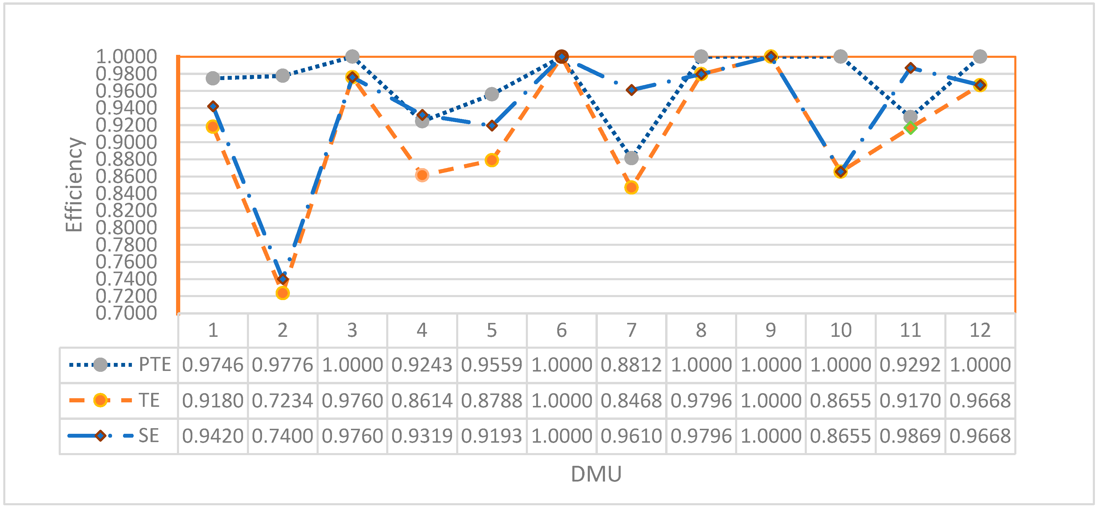
| TE | PTE | SE | ||||||||
|---|---|---|---|---|---|---|---|---|---|---|
| DMUj | ||||||||||
| 1 | 0.8746 | 0.8755 | 0.9474 | 0.8992 | 0.9785 | 0.989 | 0.9967 | 0.9881 | 0.9101 | 0.0780 |
| 2 | 0.8571 | 0.8587 | 0.9463 | 0.8874 | 0.9794 | 0.9798 | 0.9972 | 0.9855 | 0.9005 | 0.0850 |
| 3 | 0.8844 | 0.8912 | 0.9761 | 0.9172 | 0.9492 | 0.9524 | 0.9944 | 0.9653 | 0.9501 | 0.0152 |
| 4 | 0.8947 | 0.8951 | 0.9798 | 0.9232 | 0.9033 | 0.9038 | 0.9854 | 0.9308 | 0.9918 | −0.0610 |
| 5 | 0.9012 | 0.9022 | 0.9739 | 0.9258 | 0.9415 | 0.9425 | 0.9854 | 0.9565 | 0.9679 | −0.0115 |
| 6 | 0.9059 | 0.9072 | 0.9783 | 0.9305 | 0.9485 | 0.9492 | 0.9911 | 0.9629 | 0.9663 | −0.0034 |
| 7 | 0.9064 | 0.9131 | 0.9852 | 0.9349 | 0.9542 | 0.9554 | 0.9993 | 0.9696 | 0.9642 | 0.0055 |
| Average | 0.9169 | 0.9672 | 0.9501 | 0.0154 | ||||||
| DMUj | PP | DQ | IT | PQ | |||||||||
|---|---|---|---|---|---|---|---|---|---|---|---|---|---|
| Model | Data | Projection | Diff. (%) | Data | Projection | Diff. (%) | Data | Projection | Diff. (%) | Data | Projection | Diff. (%) | |
| CCR | 1 | 24,235.50 | 21,866.57 | −9.77 | 125.7777 | 94.42027 | −24.93 | 3471.387 | 1469.371 | −57.67 | 20,728.33 | 20,728.33 | 0.00 |
| 2 | 24,162.77 | 21,545.93 | −10.83 | 114.9997 | 92.20273 | −19.82 | 3801.447 | 1544.804 | −59.36 | 20,384.87 | 20,384.87 | 0.00 | |
| 3 | 23,567.83 | 21,604.67 | −8.33 | 108.2223 | 88.26153 | −18.44 | 2822.163 | 1299.394 | −53.96 | 20,889.97 | 20,889.97 | 0.00 | |
| 4 | 21,791.97 | 20,039.83 | −8.04 | 102.2222 | 82.81483 | −18.99 | 2413.11 | 366.3373 | −84.82 | 19,562.93 | 19,562.93 | 0.00 | |
| 5 | 19,452.77 | 18,090.2 | −7.00 | 98.16653 | 76.83613 | −21.73 | 1823.943 | 295.734 | −83.79 | 17,682.13 | 17,682.13 | 0.00 | |
| 6 | 18,594.60 | 17,402.13 | −6.41 | 88.05557 | 73.32023 | −16.73 | 1994.057 | 294.472 | −85.23 | 17,004.37 | 17,004.37 | 0.00 | |
| 7 | 17,736.43 | 16,618.97 | −6.30 | 105.1113 | 60.52847 | −42.41 | 2372.777 | 957.104 | −59.66 | 15,963.63 | 15,963.63 | 0.00 | |
| Average | −8.10 | −23.3 | −69.21 | 0.00 | |||||||||
| BCC | 1 | 24,235.5 | 23,862.77 | −1.54 | 125.7767 | 120.9733 | −3.82 | 3471.387 | 2509.017 | −27.72 | 20,728.33 | 21,373.13 | 3.11 |
| 2 | 24,162.77 | 23,811.93 | −1.45 | 114.9967 | 113.49 | −1.31 | 3801.447 | 2780.73 | −26.85 | 20,384.87 | 21,140.6 | 3.71 | |
| 3 | 23,567.83 | 22,715.97 | −3.61 | 108.2233 | 102.8267 | −4.99 | 2822.163 | 2194.013 | −22.26 | 20,889.97 | 20,945.23 | 0.26 | |
| 4 | 21,791.97 | 20,200.47 | −7.30 | 102.22 | 76.3 | −25.36 | 2413.11 | 1021.95 | −57.65 | 19,562.93 | 19,562.93 | 0.00 | |
| 5 | 19,452.77 | 18,472.57 | −5.04 | 98.16333 | 74.77667 | −23.82 | 1823.943 | 1076.643 | −40.97 | 17,682.13 | 17,682.13 | 0.00 | |
| 6 | 18,594.6 | 17,802.33 | −4.26 | 88.05667 | 69.47333 | −21.10 | 1994.057 | 1107.037 | −44.48 | 17,004.37 | 17,004.37 | 0.00 | |
| 7 | 17,736.43 | 17,097.87 | −3.60 | 105.1133 | 86.35333 | −17.85 | 2372.777 | 1853.293 | −21.89 | 15,963.63 | 15,963.63 | 0.00 | |
| Average | −3.83 | −14.04 | −34.55 | 1.01 | |||||||||
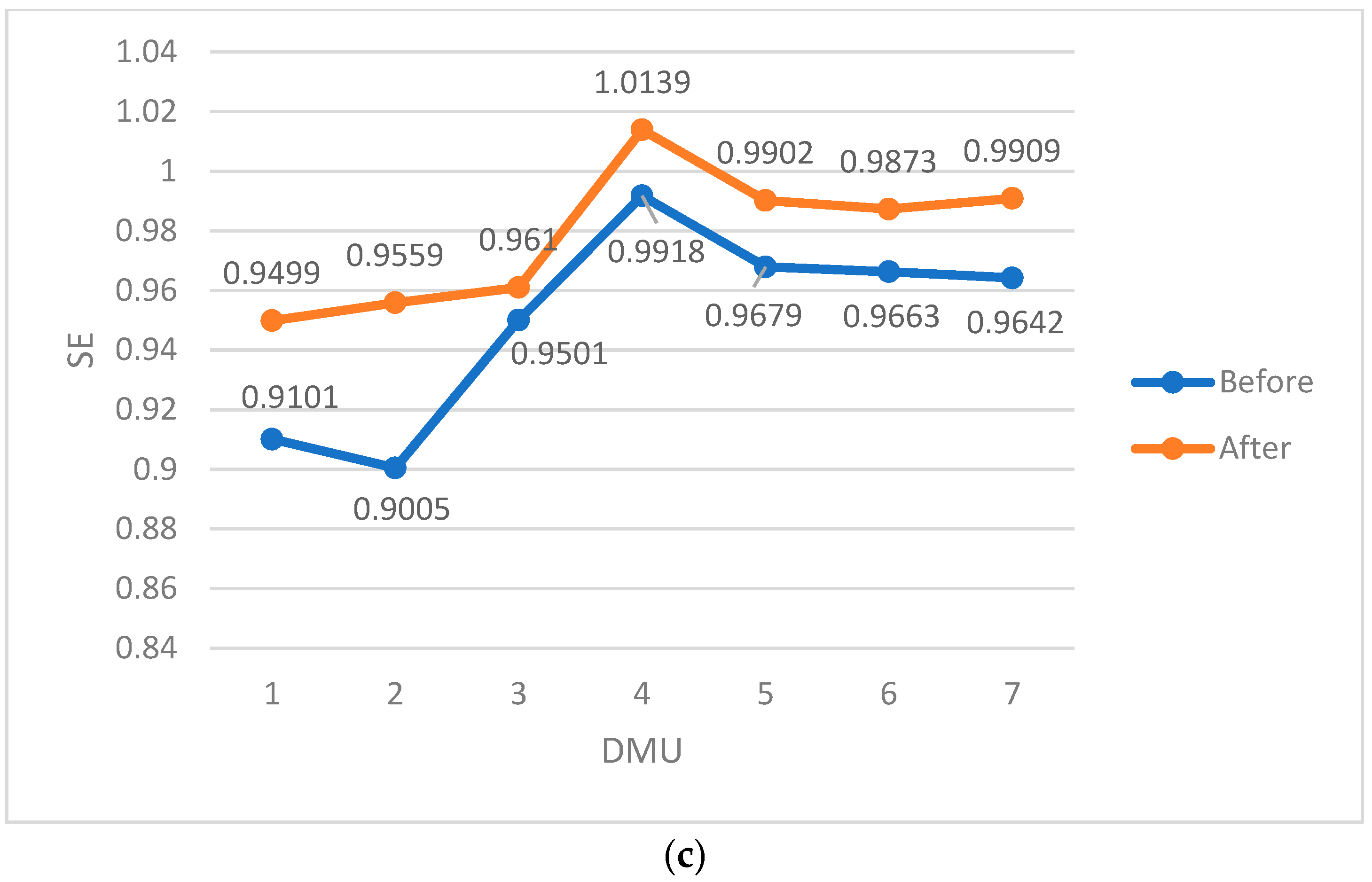
| DMUj | ||||||||||
|---|---|---|---|---|---|---|---|---|---|---|
| 1 | 0.9183 | 0.9193 | 0.9465 | 0.9280 | 0.9429 | 0.9881 | 1.0000 | 0.9770 | 0.9499 | 0.0271 |
| 2 | 0.9251 | 0.9324 | 0.9553 | 0.9376 | 0.9538 | 0.9888 | 1.0000 | 0.9809 | 0.9559 | 0.0250 |
| 3 | 0.9286 | 0.9358 | 0.9545 | 0.9396 | 0.9614 | 0.9782 | 0.9938 | 0.9778 | 0.9610 | 0.0168 |
| 4 | 0.9394 | 0.9542 | 0.9633 | 0.9523 | 0.8873 | 0.9624 | 0.9679 | 0.9392 | 1.0139 | −0.0747 |
| 5 | 0.9473 | 0.9635 | 0.9752 | 0.9620 | 0.9438 | 0.9709 | 1.0000 | 0.9716 | 0.9902 | −0.0186 |
| 6 | 0.9356 | 0.9512 | 0.9654 | 0.9507 | 0.9363 | 0.9589 | 0.9938 | 0.9630 | 0.9873 | −0.0243 |
| 7 | 0.9588 | 0.9654 | 0.9744 | 0.9662 | 0.9446 | 0.9806 | 1.0000 | 0.9751 | 0.9909 | −0.0158 |
| Averages | 0.9481 | 0.9692 | 0.9784 | |||||||
Disclaimer/Publisher’s Note: The statements, opinions and data contained in all publications are solely those of the individual author(s) and contributor(s) and not of MDPI and/or the editor(s). MDPI and/or the editor(s) disclaim responsibility for any injury to people or property resulting from any ideas, methods, instructions or products referred to in the content. |
© 2023 by the authors. Licensee MDPI, Basel, Switzerland. This article is an open access article distributed under the terms and conditions of the Creative Commons Attribution (CC BY) license (https://creativecommons.org/licenses/by/4.0/).
Share and Cite
Al-Refaie, A.; Lepkova, N. A Proposed DEA Window Analysis for Assessing Efficiency from Asymmetry Dynamic Data. Symmetry 2023, 15, 1650. https://doi.org/10.3390/sym15091650
Al-Refaie A, Lepkova N. A Proposed DEA Window Analysis for Assessing Efficiency from Asymmetry Dynamic Data. Symmetry. 2023; 15(9):1650. https://doi.org/10.3390/sym15091650
Chicago/Turabian StyleAl-Refaie, Abbas, and Natalija Lepkova. 2023. "A Proposed DEA Window Analysis for Assessing Efficiency from Asymmetry Dynamic Data" Symmetry 15, no. 9: 1650. https://doi.org/10.3390/sym15091650
APA StyleAl-Refaie, A., & Lepkova, N. (2023). A Proposed DEA Window Analysis for Assessing Efficiency from Asymmetry Dynamic Data. Symmetry, 15(9), 1650. https://doi.org/10.3390/sym15091650