Article

Semilocal Convergence of a Multi-Step Parametric Family of Iterative Methods

by
Eva G. Villalba
,
Eulalia Martínez
* and
Paula Triguero-Navarro
Multidisciplinary Institute of Mathematics, Universitat Politènica de València, 46022 València, Spain
*
Author to whom correspondence should be addressed.
Symmetry 2023, 15(2), 536; https://doi.org/10.3390/sym15020536
Submission received: 23 January 2023 / Revised: 4 February 2023 / Accepted: 13 February 2023 / Published: 17 February 2023

Abstract

:
In this paper, we deal with a new family of iterative methods for approximating the solution of nonlinear systems for non-differentiable operators. The novelty of this family is that it is a m-step generalization of the Steffensen-type method by updating the divided difference operator in the first two steps but not in the following ones. This procedure allows us to increase both the order of convergence and the efficiency index with respect to that obtained in the family that updates divided differences only in the first step. We perform a semilocal convergence study that allows us to fix the convergence domain and uniqueness for real applied problems, where the existence of a solution is not known a priori. After this study, some numerical tests are developed to apply the semilocal convergence theoretical results obtained. Finally, mediating the dynamic planes generated by the different numerical methods that compose the family, we study the symmetry of the basins of attraction generated by each solution, the shape of these basins, and the convergence to each root of a polynomial function.

1. Introduction

Using iterative methods for solving nonlinear systems is the most common technique to solve a great variety of applied nonlinear problems. Nowadays, iterative methods with a high order of convergence are being developed because the use of variable precision arithmetic in the existing software allows us to obtain approximated solutions with high accuracy. In addition, other approximation techniques have been developed in recent years, such as hybrid algorithms, schemes that use iterative methods together with optimization algorithms [1,2].
In this sense, we deal, in the present work, with high-order iterative methods for solving the system F ( x ) = 0 , with F, a nonlinear operator between Banach spaces X and Y [3,4].
It is well known that the iteration function for solving the problem involves the operator F and probably its Fréchet derivative, F ( x ) , as is the case of Newton’s method [5]. However, in real applications, it is highly probable to find non-differentiable operators modeling the problem. In these cases, the secant-type or Steffensen-type iterative methods are used [6,7,8] since the derivative has been approximated by divided differences, mainly first-order forward or backward divided differences or second-order symmetric divided differences [9]. For this reason, we concentrate on high-order iterative methods for non-differentiable problems [10]. Let us consider the composition of a generalized Steffensen method with itself by performing m steps, whose iterative expression is as follows:
z 1 ( k ) = x ( k ) [ w ( k ) , x ( k ) ; F ] 1 F ( x ( k ) ) z 2 ( k ) = z 1 ( k ) [ w ( k ) , x ( k ) ; F ] 1 F ( z 1 ( k ) ) z j ( k ) = z j 1 ( k ) [ w ( k ) , x ( k ) ; F ] 1 F ( z j 1 ( k ) ) j = 1 , 2 , , m z m 1 ( k ) = z m 2 ( k ) [ w ( k ) , x ( k ) ; F ] 1 F ( z m 2 ( k ) ) x ( k + 1 ) = z m 1 ( k ) [ w ( k ) , x ( k ) ; F ] 1 F ( z m 1 ( k ) ) , k = 0 , 1 ,
where x ( 0 ) is the starting point, w ( k ) = x ( k ) + β F ( x ( k ) ) , and β is an arbitrary constant such that β 0 . The number of steps selected is denoted by m, and k denotes which iteration we are computing. Ref. [11] proved that this iterative method reaches convergence order m + 1 (see [12,13,14]).
In order to increase the convergence order without losing the efficiency index, we introduce a new family of iterative methods, consisting in performing m-steps per iteration, but we will perform two first steps of the Steffensen method updating all data. After that, we reuse the divided differences of the second step in the remaining ones. The iterative expression is as follows:
z 1 ( k ) = x ( k ) [ w ( k ) , x ( k ) ; F ] 1 F ( x ( k ) ) z 2 ( k ) = z 1 ( k ) [ z 1 ( k ) , v ( k ) ; F ] 1 F ( z 1 ( k ) ) z j ( k ) = z j 1 ( k ) [ z 1 ( k ) , v ( k ) ; F ] 1 F ( z j 1 ( k ) ) , j = 2 , , m z m 1 ( k ) = z m 2 ( k ) [ z 1 ( k ) , v ( k ) ; F ] 1 F ( z m 2 ( k ) ) x ( k + 1 ) = z m 1 ( k ) [ z 1 ( k ) , v ( k ) ; F ] 1 F ( z m 1 ( k ) ) , k = 0 , 1 ,
where w ( k ) = x ( k ) + β F ( x ( k ) ) and v ( k ) = z 1 ( k ) + β F ( z 1 ( k ) ) . The number of steps selected is denoted by m, and k denotes which iteration we are computing. That is, we perform two steps of the Steffensen type. From then, by using the divided difference obtained in the second step, we perform m 2 new steps.
Our family of methods coincides with the family studied in [15] for the weight function H ( t ) = t 1 and for the parameters β = δ . Moreover, in this article, the complex dynamics is studied in depth. From this study, we can deduce the dynamics of our family (for example, see [16,17]).
The paper is organized as follows: Section 2 is devoted to set a semilocal convergence study for this new family of iterative methods. Next, in Section 3, we perform some numerical tests in order to apply the theoretical results obtained previously. Finally, we expose some conclusions.

2. Semilocal Convergence

In this section, we analyze the semilocal convergence of the iterative method (2), that is, we impose the necessary conditions so that, given a starting point x ( 0 ) , the iterative method (2) converges to a solution. Moreover, we determine the existence and uniqueness convergence domains [18].
For this, we consider x ( 0 ) Ω , and we assume the following:
(I)
There exists L 0 1 = L ( x ( 0 ) ) 1 = [ w ( 0 ) , x ( 0 ) ; F ] 1 such that L 0 1 γ . Furthermore, F ( x ( 0 ) ) η 0 such that L 0 1 F ( x ( 0 ) ) γ η 0 = b .
(II)
F ( x ) F ( y ) μ 0 x y , x , y Ω where μ 0 : R + R + is a continuous non-decreasing function.
(III)
We suppose that there exists [ x , y ; F ] for each pair x , y Ω , x y such that the divided differences operator satisfies the following:
[ x , y ; F ] [ u , v ; F ] μ 1 x u , y v ; for all x , y , u , v Ω ,
where μ 1 : R + × R + R + is a continuous non-decreasing function with respect to both arguments.
Note that since F is non-differentiable, μ 1 0 , 0 > 0 . Then, we will give a generalized result of the semilocal convergence. We will do so by fixing the radius r of the domain of existence and we will try to calculate it so that the sequence { x ( n ) } is contained in the ball of convergence B ( x ( 0 ) , r ) whose center is the initial iteration and whose radius is our fixed r.
Theorem 1.
Under conditions (I)–(III), we consider the following functions and parameters:
l ( t ) = μ 1 ( t , β η 0 ) , m ( t ) = γ μ 1 ( t , t + β η 0 ( t ) ) , λ ( t ) = γ 1 m ( t ) l ( t ) ,
with t R + . Suppose the following equation has at least one positive real root:
t b 1 λ ( t ) = 0 ,
where r is the smallest positive real root that satisfies Equation (3) and the conditions l ( r ) γ < 1 , m ( r ) < 1 and λ ( r ) < 1 . Then, the sequence { x n } given by the iterative method (2) is well defined, remains on the semilocal ball of convergence B ( x 0 , r ) and converges to the solution α of the equation F ( x ) = 0 .
Proof. 
To simplify the notation, we denote
L i = L ( x ( i ) ) = [ x ( i ) + β F ( x ( i ) ) , x ( i ) ; F ] .
We start from the fact that z 1 ( 0 ) is well defined since by the condition ( I ) , we have the following:
z 1 ( 0 ) x ( 0 ) = L 0 1 F ( x ( 0 ) ) γ η 0 = b < r .
Let us see that there exists [ z 1 ( 0 ) , v ( 0 ) ; F ] 1 . To do this, we denote S 0 = [ z 1 ( 0 ) , v ( 0 ) ; F ] 1 and apply Banach’s lemma:
I L 0 1 S 0 L 0 1 L 0 S 0 γ [ x ( 0 ) , x ( 0 ) + β F ( x ( 0 ) ) ; F ] [ z 1 ( 0 ) , z 1 ( 0 ) + β F ( z 1 ( 0 ) ) ; F ] γ x ( 0 ) z 1 ( 0 ) , x ( 0 ) z 1 ( 0 ) + β ( F ( x ( 0 ) ) F ( z 1 ( 0 ) ) ) γ μ 1 r , r + β μ 0 ( r ) = m ( r ) < 1 .
So, by applying Banach’s lemma, there exists S 0 1 and
S 0 1 γ 1 m ( r ) .
Since F is Fréchet differentiable, one has
F ( z 1 ( 0 ) ) = F ( z 1 ( 0 ) ) + F ( x ( 0 ) ) F ( x ( 0 ) ) = F ( x ( 0 ) ) + [ z 1 ( 0 ) , x ( 0 ) ; F ] z 1 ( 0 ) x ( 0 ) .
By the first step,
F ( x ( 0 ) ) = [ w ( 0 ) , x ( 0 ) ; F ] ( z 1 ( 0 ) x ( 0 ) ) .
Therefore,
F ( z 1 ( 0 ) ) = [ z 1 ( 0 ) , x ( 0 ) ; F ] [ x ( 0 ) , w ( 0 ) ; F ] ( z 1 ( 0 ) x ( 0 ) ) .
Taking the rules in the above expression and taking into account conditions (I)–(III), one has
F ( z 1 ( 0 ) ) μ 1 z 1 ( 0 ) x ( 0 ) , w ( 0 ) x ( 0 ) z 1 ( 0 ) x ( 0 ) μ 1 r , β η 0 z 1 ( 0 ) x ( 0 ) l ( r ) γ η 0 < η 0 ,
where we denote l ( r ) = μ 1 r , β η 0 to simplify the notation. Moreover, thanks to the condition of the theorem l ( r ) γ < 1 , we can say that l ( r ) γ η 0 < η 0 . With this bound, we can determine
z 2 ( 0 ) z 1 ( 0 ) = S 0 1 F ( z 1 ( 0 ) ) γ 1 m ( r ) l ( r ) z 1 ( 0 ) x ( 0 ) = λ ( r ) z 1 ( 0 ) x ( 0 ) < r ,
where we denote λ ( r ) = γ 1 m ( r ) l ( r ) . Moreover, in the previous equation, we applied the fact that λ ( r ) < 1 . Thus,
z 2 ( 0 ) x ( 0 ) = z 2 ( 0 ) z 1 ( 0 ) + z 1 x ( 0 ) λ ( r ) z 1 ( 0 ) x ( 0 ) + z 1 x ( 0 ) = λ ( r ) + 1 z 1 ( 0 ) x ( 0 ) ( 1 + λ ( r ) ) b < r .
Therefore, since z 2 ( 0 ) x ( 0 ) < r , one has z 2 B ( x ( 0 ) , r ) . To prove that z 3 resides inside B ( x ( 0 ) , r ) , we must first bound
z 3 ( 0 ) z 2 ( 0 ) = S 0 1 F ( z 2 ( 0 ) ) γ 1 m ( r ) F ( z 2 ( 0 ) ) .
As the value of F ( z 2 ( 0 ) ) is unknown, we are going to develop the expression
F ( z 2 ( 0 ) ) = F ( z 2 ( 0 ) ) + F ( z 1 ( 0 ) ) F ( z 1 ( 0 ) ) = F ( z 1 ( 0 ) ) + [ z 1 ( 0 ) , z 2 ( 0 ) ; F ] ( z 2 ( 0 ) z 1 ( 0 ) ) = [ z 1 ( 0 ) , v ( 0 ) ; F ] z 2 ( 0 ) z 1 ( 0 ) + [ z 2 ( 0 ) , z 1 ( 0 ) ; F ] ( z 2 ( 0 ) z 1 ( 0 ) ) .
By taking norms,
F ( z 2 ( 0 ) ) z 2 ( 0 ) z 1 ( 0 ) μ 1 z 2 ( 0 ) z 1 ( 0 ) , v ( 0 ) z 1 ( 0 ) μ 1 r , β F ( z 1 ( 0 ) ) z 2 ( 0 ) z 1 ( 0 ) μ 1 r , β η 0 z 2 ( 0 ) z 1 ( 0 ) = l ( r ) z 2 ( 0 ) z 1 ( 0 ) = l ( r ) γ η 0 < η 0 .
Now, we can bound the following z 3 ( 0 ) z 2 ( 0 ) :
z 3 ( 0 ) z 2 ( 0 ) γ 1 m ( r ) F ( z 2 ( 0 ) ) γ 1 m ( r ) l ( r ) z 2 ( 0 ) z 1 ( 0 ) λ ( r ) z 2 ( 0 ) z 1 ( 0 ) λ ( r ) 2 z 1 ( 0 ) x ( 0 ) < r .
It is therefore easy to obtain that
z 3 ( 0 ) x ( 0 ) z 3 ( 0 ) z 2 ( 0 ) + z 2 ( 0 ) z 1 ( 0 ) + z 1 ( 0 ) x ( 0 ) λ ( r ) 2 z 1 ( 0 ) x ( 0 ) + λ ( r ) z 1 ( 0 ) x ( 0 ) + z 1 ( 0 ) x ( 0 ) = λ ( r ) 2 + λ ( r ) + 1 z 1 ( 0 ) x ( 0 ) < r .
This proves that z 3 B ( x ( 0 ) , r ) . We are going to induce the number of steps m to finally obtain that the iteration x ( 1 ) is also inside the convergence ball. To do so, we assume that for q 3 , the following are satisfied:
(1)
F ( z q ( 0 ) ) l ( r ) z q ( 0 ) z q 1 ( 0 ) < η 0 .
(2)
z q ( 0 ) z q 1 ( 0 ) λ ( r ) z q 1 ( 0 ) z q 2 ( 0 ) λ ( r ) q 1 z 1 ( 0 ) x ( 0 ) < r .
(3)
z q ( 0 ) x ( 0 ) 1 λ ( r ) q 1 λ ( r ) b < r and, therefore, z q ( 0 ) B ( x ( 0 ) , r ) .
Let us see that, since it is true for q, it is also true for q + 1 .
  • We start by proving (2) for q + 1 , using (1), (2) and (3) for q:
    z q + 1 ( 0 ) z q ( 0 ) = [ z 1 ( 0 ) , v ( 0 ) ; F ] 1 F ( z q ( 0 ) ) γ 1 m ( r ) l ( r ) z q ( 0 ) z q 1 ( 0 ) λ ( r ) z q ( 0 ) z q 1 ( 0 ) λ ( r ) q z 1 ( 0 ) x ( 0 ) < r .
    It is, therefore, proven.
  • Using the hypothesis on q, we prove (3) for q + 1 :
    z q + 1 ( 0 ) x ( 0 ) = z q + 1 ( 0 ) z q ( 0 ) + z q ( 0 ) x ( 0 ) λ ( r ) q z 1 ( 0 ) x ( 0 ) + 1 λ ( r ) q 1 λ ( r ) b λ ( r ) q + 1 λ ( r ) q 1 λ ( r ) b = 1 λ ( r ) q + 1 1 λ ( r ) b < r .
    With this, it is proved that z q + 1 B ( x ( 0 ) , r ) and (3) is satisfied for q + 1 .
  • Finally we prove (1) for q + 1 provided that q < m :
    F ( z q + 1 ( 0 ) ) = F ( z q + 1 ( 0 ) ) + F ( z q ( 0 ) ) F ( z q ( 0 ) ) = [ z q + 1 ( 0 ) , z q ( 0 ) ; F ] ( z q + 1 ( 0 ) z q ( 0 ) ) + F ( z q ( 0 ) ) = [ z q + 1 ( 0 ) , z q ( 0 ) ; F ] ( z q + 1 ( 0 ) z q ( 0 ) ) [ z 1 ( 0 ) , v ( 0 ) ; F ] ( z q + 1 ( 0 ) z q ( 0 ) ) .
    Applying the rules, we obtain
    F ( z q + 1 ( 0 ) ) μ 1 z q + 1 ( 0 ) z 1 ( 0 ) , z q ( 0 ) v ( 0 ) z q + 1 ( 0 ) z q ( 0 ) μ 1 z q + 1 ( 0 ) x ( 0 ) + x ( 0 ) z 1 ( 0 ) , z q ( 0 ) z 1 ( 0 ) + β F ( z 1 ( 0 ) ) z q + 1 ( 0 ) z q ( 0 ) μ 1 1 λ ( r ) q + 1 1 λ ( r ) b + b , 1 λ ( r ) q 1 λ ( r ) b + b + β η 0 z q + 1 ( 0 ) z q ( 0 ) l ( r ) z q + 1 ( 0 ) z q ( 0 ) ,
    where
    l ( r ) = m a x μ 1 r , β η 0 , μ 1 2 b b λ ( r ) λ ( r ) q + 1 1 λ ( r ) , 2 b b λ ( r ) λ ( r ) q 1 + 1 1 λ ( r ) + β η 0 ,
    for q = 2 , , m 1 . Therefore, it is proved (3) for q + 1 .
If q = m 1 , we have that z m ( 0 ) = x ( 1 ) and, therefore, the first iteration generated by the method is inside B ( x ( 0 ) , r ) . Now we want to prove that x ( 2 ) B ( x ( 0 ) , r ) . To do so, we have to see that z 1 ( 1 ) , , z m ( 1 ) are well defined and inside the convergence ball. Since z m ( 0 ) = x ( 1 ) B ( x ( 0 ) , r ) , we go to the first step of the method. In this step, we want to bound z 1 ( 1 ) x ( 1 ) to prove that x ( 1 ) is inside B ( x ( 0 ) , r ) . By the method, one has
z 1 ( 1 ) x ( 1 ) [ w ( 1 ) , x ( 1 ) ; F ] 1 F ( x ( 1 ) ) L 1 1 F ( x ( 1 ) ) .
Since by induction we saw that (3) is satisfied for q 3 , then
z 1 ( 1 ) x ( 1 ) L 1 1 l ( r ) z m ( 0 ) z m 1 ( 0 ) .
Now, let us see that L 1 1 exists. To do this, we use Banach’s lemma:
I L 0 1 L 1 L 0 1 L 0 L 1 γ [ w ( 0 ) , x ( 0 ) ; F ] [ w ( 1 ) , x ( 1 ) ; F ] γ μ 1 w ( 1 ) w ( 0 ) , x ( 1 ) x ( 0 ) γ μ 1 x ( 1 ) x ( 0 ) + β ( F ( x ( 1 ) ) F ( x ( 0 ) ) , x ( 1 ) x ( 0 ) γ μ 1 x ( 1 ) x ( 0 ) + β μ 0 x ( 1 ) x ( 0 ) , x ( 1 ) x ( 0 ) γ μ 1 r + β μ 0 ( r ) , r = m ( r ) < 1 .
Therefore, by Banach’s lemma,
L 1 1 γ 1 m ( r ) .
Therefore,
z 1 ( 1 ) x ( 1 ) γ 1 m ( r ) l ( r ) z m ( 0 ) z m 1 ( 0 ) λ ( r ) z m ( 0 ) z m 1 ( 0 ) λ ( r ) λ ( r ) m 1 z 1 ( 0 ) x ( 0 ) λ ( r ) m z 1 ( 0 ) x ( 0 ) < r .
To see if it is part of the convergence ball,
z 1 ( 1 ) x ( 0 ) z 1 ( 1 ) x ( 1 ) + x ( 1 ) x ( 0 ) λ ( r ) m z 1 ( 0 ) x ( 0 ) + z m ( 0 ) x ( 0 ) λ ( r ) m + 1 λ ( r ) m 1 λ ( r ) z 1 ( 0 ) x ( 0 ) = 1 λ ( r ) m + 1 1 λ ( r ) b < r .
It is therefore established that z 1 ( 1 ) B ( x ( 0 ) , r ) . To continue with induction, we are going to prove that z 2 ( 1 ) is inside the convergence ball. To do this, we want to bound
z 2 ( 1 ) z 1 ( 1 ) [ z 1 ( 1 ) , v ( 1 ) ; F ] 1 F ( z 1 ( 1 ) ) S 1 1 F ( z 1 ( 1 ) ) .
Let see that there exists S 1 1 using Banach’s lemma
I L 0 1 S 1 L 0 1 L 0 S 1 γ [ w ( 0 ) , x ( 0 ) ; F ] [ v ( 1 ) , z 1 ( 1 ) ; F ] γ μ 1 z 1 ( 1 ) x ( 0 ) + β F ( z 1 ( 1 ) ) F ( x ( 0 ) ) , z 1 ( 1 ) x ( 0 ) γ μ 1 r + β μ 0 ( r ) , r = m ( r ) < 1 .
Therefore, there exists S 1 1 and S 1 1 γ 1 m ( r ) . Now we develop
F ( z 1 ( 1 ) ) = F ( z 1 ( 1 ) ) + F ( x ( 1 ) ) F ( x ( 1 ) ) = [ z 1 ( 1 ) , x ( 1 ) ; F ] ( z 1 ( 1 ) x ( 1 ) ) + F ( x ( 1 ) ) .
By taking the norms, we obtain
F ( z 1 ( 1 ) ) [ z 1 ( 1 ) , x ( 1 ) ; F ] ( z 1 ( 1 ) x ( 1 ) ) [ x ( 1 ) , w ( 1 ) ; F ] ( z 1 ( 1 ) x ( 1 ) ) μ 1 z 1 ( 1 ) x ( 1 ) , β F ( x ( 1 ) ) z 1 ( 1 ) x ( 1 ) μ 1 z 1 ( 1 ) x ( 1 ) , β η 0 z 1 ( 1 ) x ( 1 ) S z 1 ( 1 ) x ( 1 ) < η 0 .
Therefore, we calculate the difference
z 2 ( 1 ) z 1 ( 1 ) γ 1 m ( r ) l ( r ) z 1 ( 1 ) x ( 1 ) λ ( r ) z 1 ( 1 ) x ( 1 ) λ ( r ) λ ( r ) m z 1 ( 0 ) x ( 0 ) λ ( r ) m + 1 z 1 ( 0 ) x ( 0 ) < r .
Finally, we would have that z 2 ( 1 ) B ( x ( 0 ) , r ) , since
z 2 ( 1 ) x ( 0 ) z 2 ( 1 ) z 1 ( 1 ) + z 1 ( 1 ) x ( 0 ) λ ( r ) m + 1 z 1 ( 0 ) x ( 0 ) + 1 λ ( r ) m + 1 1 λ ( r ) z 1 ( 0 ) x ( 0 ) 1 λ ( r ) m + 2 1 λ ( r ) b < r .
Again, by induction on the number of steps to reach the iteration x ( 2 ) , we can argue analogously (1), (2) and (3) and we obtain for q = 3 , , m :
(4)
F ( z q ( 1 ) ) l ( r ) z q ( 1 ) z q 1 ( 1 ) η 0 .
(5)
z q ( 1 ) z q 1 ( 1 ) λ ( r ) z q 1 ( 1 ) z q 2 ( 1 ) λ ( r ) m + q 1 z 1 ( 0 ) x ( 0 ) < r .
(6)
z q ( 1 ) x ( 0 ) 1 λ ( r ) m + q 1 λ ( r ) b < r and, therefore, z q ( 1 ) B ( x ( 0 ) , r ) .
By induction, we would see that (4), (5) and (6) are satisfied for q = m . Therefore, x ( 2 ) = z m ( 1 ) is well defined, and it holds that x ( 2 ) B ( x ( 0 ) , r ) . Suppose we repeat the process to see that there exist x ( 1 ) and x ( 2 ) for all the iterations x ( i ) with i = 3 , , n 1 . Then, we would obtain the following:
(7)
F ( z q ( n 1 ) ) l ( r ) z q ( n 1 ) z q 1 ( n 1 ) η 0 for q = 2 , , m and F ( z 1 ( n 1 ) ) l ( r ) z 1 ( n 1 ) x ( n 1 ) η 0 .
(8)
z q ( n 1 ) z q 1 ( n 1 ) λ ( r ) z q 1 ( n 1 ) z q 2 ( n 1 ) λ ( r ) ( n 1 ) m + q 1 z 1 ( 0 ) x ( 0 ) < r for q = 1 , , m .
(9)
z q ( n 1 ) x ( 0 ) 1 λ ( r ) ( n 1 ) m + q 1 λ ( r ) b < r and z q ( n 1 ) B ( x ( 0 ) , r ) for q = 1 , , m where z m ( n 1 ) = x ( n ) .
Assuming that (7), (8) and (9) are satisfied for n 1 , then let us prove that they are also satisfied for n, and, furthermore, x ( n + 1 ) is well defined and belongs to B ( x ( 0 ) , r ) . We start with the same aim as always. We want to bound
z 1 ( n ) x ( n ) [ w ( n ) , x ( n ) ; F ] 1 F ( x ( n ) ) L n 1 F ( x ( n ) ) .
To do this, we must prove that there exists L n 1 :
I L 0 1 L n L 0 1 L 0 L n γ [ w ( 0 ) , x ( 0 ) ; F ] [ w ( n ) , x ( n ) ; F ] γ μ 1 w ( 0 ) w ( n ) , x ( n ) x ( 0 ) γ μ 1 x ( n ) x ( 0 ) + β F ( x ( n ) ) F ( x ( 0 ) ) , r γ μ 1 r + β μ 0 ( r ) , r = m ( r ) < 1 .
Therefore, applying Banach’s lemma again, we obtain that there exists L n 1 and L n 1 γ 1 m ( r ) . As we have seen in induction,
F ( x ( n ) ) l ( r ) z m ( n 1 ) z m 1 ( n 1 ) < η 0 .
Thus,
z 1 ( n ) x ( n ) γ 1 m ( r ) l ( r ) z m ( n 1 ) z m 1 ( n 1 ) λ ( r ) z m ( n 1 ) z m 1 ( n 1 )
By applying (8), we obtain
z 1 ( n ) x ( n ) λ ( r ) λ ( r ) ( n 1 ) m + m 1 z 1 ( 0 ) x ( 0 ) λ ( r ) n m z 1 ( 0 ) x ( 0 ) < r .
From this, we deduce
z 1 ( n ) x ( 0 ) z 1 ( n ) x ( n ) + x ( n ) x ( 0 ) λ ( r ) n m z 1 ( 0 ) x ( 0 ) + x ( n ) x ( 0 ) .
By applying (9), we easily obtain
z 1 ( n ) x ( 0 ) λ ( r ) n m z 1 ( 0 ) x ( 0 ) + 1 λ ( r ) m ( n 1 ) + m 1 λ ( r ) z 1 ( 0 ) x ( 0 ) 1 λ ( r ) n m + 1 1 λ ( r ) z 1 ( 0 ) x ( 0 ) 1 λ ( r ) n m + 1 1 λ ( r ) b < r ,
that is, z 1 ( n ) B ( x ( 0 ) , r ) . Let us see that z 2 ( n ) B ( x ( 0 ) , r ) . To do this, we first bound
z 2 ( n ) z 1 ( n ) [ z 1 ( n ) , v ( n ) ; F ] 1 F ( z 1 ( n ) ) S n 1 F ( z 1 ( n ) ) .
Let see that S n 1 exists, using Banach’s lemma:
I L 0 1 S n L 0 1 L 0 S n γ [ w ( 0 ) , x ( 0 ) ; F ] [ v ( n ) , z 1 ( n ) ; F ] γ μ 1 z 1 ( n ) x ( 0 ) , z 1 ( n ) x ( 0 ) + β F ( z 1 ( n ) ) F ( x ( 0 ) ) γ μ 1 r , r + β μ 0 ( r ) = m ( r ) < 1 .
Therefore, there exists S n 1 , and S n 1 γ 1 m ( r ) . Now, we calculate
F ( z 1 ( n ) ) = F ( x ( n ) ) + [ z 1 ( n ) , x ( n ) ; F ] ( z 1 ( n ) x ( n ) ) = [ x ( n ) , z 1 ( n ) ; F ] [ w ( n ) , x ( n ) ; F ] ( z 1 ( n ) x ( n ) ) ,
and by applying rules
F ( z 1 ( n ) ) z 1 ( n ) x ( n ) μ 1 β F ( x ( n ) ) , z 1 ( n ) x ( n ) z 1 ( n ) x ( n ) μ 1 r , β η 0 l ( r ) z 1 ( n ) x ( n ) < η 0 .
Therefore, we calculate the distance between iterations
z 2 ( n ) z 1 ( n ) γ 1 m ( r ) l ( r ) z 1 ( n ) x ( n ) λ ( r ) m n + 1 z 1 ( 0 ) x ( 0 ) < r .
Then, we have that z 2 ( n ) B ( x ( 0 ) , r ) , since
z 2 ( n ) x ( 0 ) z 2 ( n ) z 1 ( n ) + z 1 ( n ) x ( 0 ) λ ( r ) m n + 1 z 1 ( 0 ) x ( 0 ) + 1 λ ( r ) m n + 1 1 λ ( r ) b λ ( r ) m n + 1 b + 1 λ ( r ) m n + 1 1 λ ( r ) b 1 λ ( r ) m n + 2 1 λ ( r ) b < r .
By induction on the number of steps in iteration number n + 1 of the method, we can reason analogously to the other iterations and obtain
(A)
F ( z m ( n ) ) l ( r ) z m ( n ) z m 1 ( n ) < η 0 .
(B)
z m ( n ) z m 1 ( n ) λ ( r ) m ( n + 1 ) 1 z 1 ( 0 ) x ( 0 ) < r .
(C)
z m ( n ) x ( 0 ) 1 λ ( r ) m ( n + 1 ) 1 λ ( r ) b < r and z m ( n ) B ( x ( 0 ) , r ) , n N .
Since x ( n + 1 ) = z m ( n ) , we obtain that the iteration x ( n + 1 ) belongs to the convergence ball B ( x 0 , r ) , where
x ( n + 1 ) x ( 0 ) b 1 λ ( r ) = r ,
being that r is the radius of convergence. Now, using (A), (B) and (C), we are going to prove that the sequence of iterations { x n } is a Cauchy sequence in the ball B ( x 0 , r ) . We want to bound x ( n ) x ( n 1 ) in relation to z 1 ( n 1 ) x ( n 1 ) .
x ( n ) x ( n 1 ) = z m ( n 1 ) x ( n 1 ) = z m ( n 1 ) z m 1 ( n 1 ) + z m 1 ( n 1 ) z m 2 ( n 1 ) + z m 2 ( n 1 ) + z 2 ( n 1 ) + z 2 ( n 1 ) z 1 ( n 1 ) + z 1 ( n 1 ) x ( n 1 ) z m ( n 1 ) z m 1 ( n 1 ) + z m 1 ( n 1 ) z m 2 ( n 1 ) + + z 2 ( n 1 ) z 1 ( n 1 ) + z 1 ( n 1 ) x ( n 1 )
By condition ( 8 ) , it follows that
z q ( n 1 ) z q 1 ( n 1 ) λ ( r ) q 1 z 1 ( n 1 ) x ( n 1 ) .
Therefore, by applying this,
x ( n ) x ( n 1 ) = z m ( n 1 ) x ( n 1 ) z m ( n 1 ) z m 1 ( n 1 ) + z m 1 ( n 1 ) z m 2 ( n 1 ) + + z 2 ( n 1 ) z 1 ( n 1 ) + z 1 ( n 1 ) x ( n 1 ) λ ( r ) m 1 z 1 ( n 1 ) x ( n 1 ) + λ ( r ) m 2 z 1 ( n 1 ) x ( n 1 ) + + λ ( r ) z 1 ( n 1 ) x ( n 1 ) + z 1 ( n 1 ) x ( n 1 ) ( λ ( r ) m 1 + λ ( r ) m 2 + + λ ( r ) + 1 ) z 1 ( n 1 ) x ( n 1 ) 1 λ ( r ) m 1 λ ( r ) z 1 ( n 1 ) x ( n 1 ) .
We therefore calculate
x ( n + k ) x ( n 1 ) x ( n + k ) x ( n + k 1 ) + x ( n + k 1 ) x ( n + k 2 ) + + x ( n + 1 ) x ( n ) + x ( n ) x ( n 1 ) 1 λ ( r ) m 1 λ ( r ) z 1 ( n + k 1 ) x ( n + k 1 ) + 1 λ ( r ) m 1 λ ( r ) z 1 ( n + k 2 ) x ( n + k 2 ) + + 1 λ ( r ) m 1 λ ( r ) z 1 ( n 1 ) x ( n 1 ) 1 λ ( r ) m 1 λ ( r ) ( z 1 ( n + k 1 ) x ( n + k 1 ) + z 1 ( n + k 2 ) x ( n + k 2 ) + + z 1 ( n 1 ) x ( n 1 ) )
Furthermore, from the property ( 8 ) it also follows that
z 1 ( n 1 ) x ( n 1 ) λ ( r ) m k z 1 ( n 1 k ) x ( n 1 k ) .
In this way,
x ( n + k ) x ( n 1 ) 1 λ ( r ) m 1 λ ( r ) ( z 1 ( n + k 1 ) x ( n + k 1 ) + z 1 ( n + k 2 ) x ( n + k 2 ) + + z 1 ( n 1 ) x ( n 1 ) ) 1 λ ( r ) m 1 λ ( r ) ( λ ( r ) m k z 1 ( n 1 ) x ( n 1 ) + λ ( r ) m ( k 1 ) z 1 ( n 1 ) x ( n 1 ) + + z 1 ( n 1 ) x ( n 1 ) ) 1 λ ( r ) m 1 λ ( r ) ( λ ( r ) m k + λ ( r ) m ( k 1 ) + + λ ( r ) m + 1 ) z 1 ( n 1 ) x ( n 1 ) 1 λ ( r ) m 1 λ ( r ) 1 λ ( r ) m ( k + 1 ) 1 λ ( r ) m z 1 ( n 1 ) x ( n 1 ) 1 λ ( r ) m 1 λ ( r ) 1 λ ( r ) m ( k + 1 ) 1 λ ( r ) m λ ( r ) m ( n 1 ) z 1 ( 0 ) x ( 0 ) 1 λ ( r ) m ( k + 1 ) 1 λ ( r ) 1 λ ( r ) m 1 λ ( r ) m λ ( r ) m ( n 1 ) z 1 ( 0 ) x ( 0 ) 1 λ ( r ) m ( k + 1 ) 1 λ ( r ) λ ( r ) m ( n 1 ) z 1 ( 0 ) x ( 0 ) < 1 1 λ ( r ) λ ( r ) m ( n 1 ) z 1 ( 0 ) x ( 0 ) .
By condition (A), F ( z m ( n ) ) l ( r ) z m ( n ) z m 1 ( n ) < η 0 .
Therefore, by applying condition (B), F ( x ( n + 1 ) ) = F ( z m ( n ) ) l ( r ) z m ( n ) z m 1 ( n ) l ( r ) λ ( r ) m 1 z 1 ( n ) x ( n ) .
Moreover, by taking limits when n , as z 1 ( n ) x ( n ) 0 , and thus, by the continuity of the operator F, F ( x * ) = 0 . □
Theorem 2.
Under the conditions (I)–(III), we suppose that the equation
γ μ 1 ( t , t + β μ 0 ( t ) ) 1 = 0
has at least one positive real root, where R is the smallest positive real root of this equation. Then, the solution α is the only solution of the equation H ( x ) = 0 in B ( α , R ) ¯ Ω
Proof. 
To see the uniqueness of the solution, we assume by the reduction to the absurd that another solution exists α ˜ B ( x 0 , R ) ¯ Ω , and we consider the operator P = [ α , α ˜ ; F ] . Then, since P ( α ˜ α ) = F ( α ˜ ) F ( α ) = 0 , if we prove that P is an inverse operator, we will have that α ˜ = α . Then, to apply Banach’s lemma, we prove
I L 0 1 P L 0 1 L 0 P γ [ x ( 0 ) , x ( 0 ) + β F ( x ( 0 ) ) ; F ] [ α , α ˜ ; F ] γ μ 1 ( x ( 0 ) α , x ( 0 ) + β F ( x ( 0 ) ) α ˜ ) γ μ 1 ( x ( 0 ) α , x ( 0 ) α ˜ + β F ( x ( 0 ) ) ) γ μ 1 ( x ( 0 ) α , x ( 0 ) α ˜ + β μ 0 ( x ( 0 ) α ) ) < γ μ 1 ( R , R + β μ 0 ( R ) ) = 1 .
In the last inequality, we used the hypothesis that there is at least one positive real root of Equation (5) since this implies that at least one of the functions μ 0 ( t ) or μ 1 ( t ) is strictly increasing. So, the uniqueness follows. □

3. Numerical Experiments

In this section, we study numerically our family of methods (2) for different values of β . In doing so, we highlight the best methods of the family from two essential points of view in numerical analysis: semi-local and dynamic convergence.
For the calculations and dynamical planes, we used MATLAB R2022a with 100-digit variable precision arithmetic.

3.1. Numerical Study of Semilocal Convergence

In this subsection, we apply the theoretical results obtained in previous sections for obtaining the convergence and uniqueness domain of the solution of a nonlinear and non-differentiable integral equation. These kinds of equations play an important role in the study of nonlinear physical phenomena that appear in various scientific and engineering fields, such as chemical physics, fluid mechanics, plasma physics, biology, etc.
We consider the equation
x ( s ) = f ( s ) + 1 2 a b K ( s , t ) ϕ ( x ( t ) ) d t , a s b ,
where K : [ a , b ] × [ a , b ] R is the Green’s function. We transform the equation by discretization into
F ( x ) ( s ) = x ( s ) f ( s ) 1 2 a b K ( s , t ) ϕ ( x ( t ) ) d t = 0 .
This problem is finite dimensional if we approximate the integral by the Gauss–Legendre quadrature formula
a b q ( t ) d t i = 1 p ω i q ( t i )
where the nodes t i and the weights ω i are known.
If we denote the approximations of x ( t i ) and f ( t i ) by x i and f i , respectively, with i = 1 , , p , then Equation (7) is equivalent to the following nonlinear system:
x i = f i + 1 2 j = 1 p a i j ϕ ( x j ) , j = 1 , , p ,
where
a i j = ω j K ( t i , t j ) = ω j ( b t i ) ( t j a ) b a , j i ω j ( b t j ) ( t i a ) b a , j i .
Now, the system (8) can be written as
F ( x ) x f 1 2 A z = 0 , F : R p R p ,
where
x = ( x 1 , , x p ) T , f = ( f 1 , , f p ) T , A = ( a i j ) i , j = 1 p , z = ( ϕ ( x 1 ) , , ϕ ( x p ) ) T .
We choose a = 0 , b = 1 , K ( s , t ) as the Green’s function in [ 0 , 1 ] × [ 0 , 1 ] and ϕ ( x ( t ) ) = ( x ( t ) ) 3 + | x ( t ) | in (6). Then, the nonlinear equation system given in (9) is of the form
F ( x ) x f 1 2 A ( x 1 3 + | x 1 | , , x p 3 + | x p | ) = 0 .
It is obvious that the function F defined in (10) is non-linear and non-differentiable. Therefore, we can apply our method which dispenses with derivatives and uses divided differences. We can consider the first-order divided differences that do not require F to be differentiable (see [11]), defined by the following expression:
[ u , v ; F ] = ( [ u , v , F ] i j ) i , j = 1 p L ( R p , R p ) , where [ u , v ; F ] i , j = 1 u j v j ( F i ( u 1 , , u j , v j + 1 , , v p ) F i ( u 1 , , u j 1 , v j , , v p ) ) , where u = ( u 1 , , u p ) T and v = ( v 1 , , v p ) T .
To simplify the problem, we consider f = 0 in (10). Obviously, in this case, α = 0 is a solution of F ( x ) = 0 , and it is the solution on which we study the semilocal convergence. Although for this study it is not necessary to know the solution, we use this information to take the Ω = B ( 0 , ξ ) as the domain.
Taking f = 0 , the nonlinear equation system given by (10) is of the form
F ( x ) = x 1 2 A z , z j = x j 3 + | x j | , j = 1 , , p .
We now calculate [ x , y ; F ] , first calculating [ x , y , F ] i j for i , j = 1 , , p :
[ x , y , F ] i j = 1 x j y j F i ( x 1 , , x j , y j + 1 , , y p ) F i ( x 1 , , x j 1 , y j , , y p ) = 1 2 ( x j y j ) ( a i 1 , , a i n ) x 1 3 + | x 1 | , , x j 3 + | x j | , y j + 1 3 + | y j + 1 | , , y p 3 + | y p | + 1 2 ( x j y j ) ( a i 1 , , a i n ) x 1 3 + | x 1 | , , x j 1 3 + | x j 1 | , y j 3 + | y j | , , y p 3 + | y p |
Since j is the only component that does not cancel out,
[ x , y , F ] i j = a i j 1 2 ( x j y j ) x j 3 + | x j | y j 3 + | y j | = a i j 2 x j 3 y j 3 x j y j + | x j | | y j | x j y j = a i j 2 ( x j 2 + x j y j + y j 2 ) + | x j | | y j | x j y j .
Therefore,
[ x , y , F ] = I 1 2 A · D i a g x 1 2 + x 1 y 1 + y 1 2 x p 2 + x p y p + y p 2 + | x 1 | | y 1 | x 1 y 1 | x p | | y p | x p y p .
If we consider Ω = B ( 0 , ξ ) , then
F ( x ) F ( y ) x y 1 2 A ( x 3 y 3 ) 1 2 A ( | x | | y | ) x y + 1 2 A x 3 y 3 + 1 2 A | x | | y | .
As we know that x 3 y 3 x y x 2 + x y + y 2 and | x | | y | x y is satisfied, then
F ( x ) F ( y ) x y + 1 2 A x y x 2 + x y + y 2 + x y x y + 1 2 A 3 ξ 2 x y + x y μ 0 ( x y ) ,
with μ 0 ( t ) = t + 1 2 A ( 3 ξ 2 + 1 ) t .
On the other hand, we develop
[ x , y ; F ] [ u , v ; F ] = I 1 2 A ( x 2 + x y + y 2 ) + | x | | y | x y I + 1 2 A ( u 2 + u v + v 2 ) + | u | | v | u v 1 2 A x 2 + x y + y 2 u 2 u v v 2 + | x | | y | x y | u | | v | u v 1 2 A x 2 u 2 + y 2 v 2 + x y u v + 2 A 1 2 A x u x + u + y v y + v + x y x v + x v u v + 2 A 1 2 A 2 ξ x u + 2 ξ | y v + x y v + v x u + 2 A 1 2 A 2 + 3 ξ ( x u + y v ) .
Therefore, we have
μ 1 ( s , t ) = 1 2 A ( 2 + 3 ξ ( s + t ) ) .
Under these conditions, α = 0 is a solution of the problem. Furthermore, assuming that the dimension of the problem is p = 8 , we have
I L I [ w ( 0 ) , x ( 0 ) ; F ] 1 2 A ( 3 ξ 2 + 1 )
since
[ w ( 0 ) , x ( 0 ) , F ] = I 1 2 A · D i a g ( x 1 ( 0 ) ) 2 + x 1 ( 0 ) w 1 ( 0 ) + ( w 1 ( 0 ) ) 2 ( x p ( 0 ) ) 2 + x p ( 0 ) w p ( 0 ) + ( w p ( 0 ) ) 2 + | x 1 ( 0 ) | | w 1 ( 0 ) | x 1 ( 0 ) w 1 ( 0 ) | x p ( 0 ) | | w p ( 0 ) | x p ( 0 ) w p ( 0 ) .
and w ( 0 ) , x ( 0 ) B ( 0 , ξ ) . Then, if 1 2 A ( 3 ξ 2 + 1 ) < 1 , by the Banach’s lemma, L 1 exists and
L 1 < 2 2 A ( 3 ξ 2 + 1 ) = γ .
For this experiment, we consider that ξ = 1 and, therefore, we take an initial estimate belonging to the ball B ( 0 , 1 ) . For example,
x ( 0 ) = ( 0.1 , , 0.1 ) T .
In this case, w ( 0 ) = x ( 0 ) + F ( x ( 0 ) ) also remains inside B ( 0 , 1 ) because
w ( 0 ) = x ( 0 ) + F ( x ( 0 ) ) x ( 0 ) + x ( 0 ) + 1 2 A ( x ( 0 ) 3 + x ( 0 ) ) 0.2063 .
In addition, in the previous bound, we used that
F ( x ( 0 ) ) x ( 0 ) + 1 2 A ( x ( 0 ) 3 + x ( 0 ) ) ,
which allows us to deduce the parameter η 0 as F ( x ( 0 ) ) 0.1063 = η 0 . The rest of the bounds and parameters are deduced for particular β , and that is the reason that in the following table, we present the radius of convergence and uniqueness that we obtain by changing β , and, in turn, we check the values of m ( r ) , λ ( r ) , b and l ( r ) γ to verify that the conditions of the semilocal convergence existence theorem are fulfilled.
As we can see in Table 1, the best semilocal convergence results are obtained for the smallest values of β . Moreover, for this value of x 0 , we also obtain a larger uniqueness radius than for the rest of the values, which implies that we can ensure the uniqueness of the solution in a larger set. On the other hand, it is interesting to note that for β = 1 , i.e., for the Steffensen multistep method with second frozen divided difference, we do not obtain the best results in terms of semilocal convergence, and this fact implies that we have better options in this new family. Finally, it is important to point out that the optimal existence and uniqueness radii are obtained when β 0 since the symmetric divided difference operators, [ x ( k ) , x ( k ) ; F ] and [ z 1 ( k ) , z 1 ( k ) ; F ] , are the best approximations to the derivatives in the (2) scheme.

3.2. Dynamical Planes for Different Steps

In this section, we compare the different dynamical planes that are generated by varying the parameter β and the number of steps m of the family of numerical methods. For dynamical planes, we choose a mesh of 400 × 400 points, and what we do is apply our family of methods to each of these points, taking the point as the method’s initial estimate z. We consider z as a complex number, and represent their real part in the abscissa axis and their imaginary part in the ordinate axis. We define that the maximum number of iterations that we must carry out with each initial estimate is 50 and we consider that the initial points of the mesh converge to one of the solutions of the function if the distance to that solution is less than 10 3 .
The function to which we apply the family of methods is
f ( x ) = x 4 1 .
We represent in orange the initial points that converge to the root 1, in green the initial points that converge to the root 1 , in blue the initial points that converge to the root i, in purple the initial points that converge to the root i and in black the initial points that do not converge to any root in fewer than 50 iterations.
As is illustrated in the dynamic planes, Figure 1, we observe a behavior similar to what happened in the numerical example of the semilocal convergence since, as the value of parameter β decreases, the basins of attraction of the roots increase. Note that when β = 0.01 , in the dynamic planes we can observe that the basins of attraction of the four roots of the function present a symmetry, that is to say, the same amount of initial points converge to the roots within the chosen mesh.
On the other hand, regarding the number of steps, using one or two steps does not apparently change the number of points that converge to a solution but it does decrease when the number of steps increases. However, by employing more steps, convergence is realized in a smaller number of iterations as we see in the figures since the intensity of color determines the number of iterations needed to satisfy the stopping criterion.
Therefore, if we had to choose between the illustrated methods, which of them is more convenient in this simple polynomial case, dynamically speaking, we would choose the method using m = 2 and β = 0.01 since it obtains a large number of points converging to one of the solutions in a few iterations.

4. Conclusions

In this work, a new family of Steffensen-type methods was introduced, and a semilocal convergence study of this family was developed. Theoretical studies of the semilocal convergence were verified by applying the method to a Hammerstein-type nonlinear integral equation. Finally, we analyzed some dynamical planes of the method applied to a nonlinear equation in order to conclude which number of steps and which β is more convenient from the dynamic point of view.
In conclusion, it is important to emphasize that, although working with methods with many steps is not convenient to study simple numerical examples, it is necessary to use these methods for problems in which we work on very large systems. This is because the more steps there are in the method used, the fewer iterations it performs to find the solution, and, therefore, this means less execution time.

Author Contributions

Conceptualisation, P.T.-N.; methodology, E.G.V., E.M. and P.T.-N.; software, E.G.V. and P.T.-N.; validation, E.G.V., E.M. and P.T.-N.; formal analysis, E.G.V. and P.T.-N.; research, E.G.V., E.M. and P.T.-N.; resources, E.G.V. and P.T.-N. research, E.G.V., E.M. and P.T.-N.; resources, E.G.V., E.M. and P.T.-N.; data preservation, E.G.V., E.M. and P.T.-N.; writing—preparation of the original draft, E.G.V., E.M. and P.T.-N.; writing—preparation of the original draft, E.G.V. and P.T.-N.; writing—revision and editing, E.G.V., E.M. and P.T.-N.; visualisation, E.G.V., E.M. and P.T.-N.; supervision, E.G.V. and E.M.; project administration, E.M.; securing funding, E.M. All authors have read and accepted the published version of the manuscript.

Funding

This research was partially supported by Grant PGC2018-095896-B-C22, funded by MCIN/AEI/10.13039/5011000113033 by “ERDF A way of making Europe”, European Union; and also partially supported by Universitat Politècnica de València Contrato Predoctoral PAID-01-20-17 (UPV).

Data Availability Statement

Data sharing not applicable.

Conflicts of Interest

The authors declare no conflict of interest.

References

  1. Sihwail, R.; Solaiman, O.S.; Ariffin, K.A.Z. New robust hybrid Jarratt-Butterfly optimization algorithm for nonlinear models. J. King Saud Univ. Comput. Inf. Sci. 2022, 34, 8207–8220. [Google Scholar] [CrossRef]
  2. Sihwail, R.; Solaiman, O.S.; Omar, K.; Ariffin, K.A.Z.; Alswaitti, M.; Hashim, I. A Hybrid Approach for Solving Systems of Nonlinear Equations Using Harris Hawks Optimization and Newton’s Method. IEEE Access 2021, 9, 95791–95807. [Google Scholar] [CrossRef]
  3. Ostrowski, A.M. Solutions of Equations in Euclidean and Banach Spaces; Academic Press: New York, NY, USA, 1973. [Google Scholar]
  4. Traub, J.F. Iterative Methods for the Solution of Equations; Prentice-Hall: Englewood Cliffs, NJ, USA, 1964. [Google Scholar]
  5. Argyros, I.K. On a theorem of L. V. Kantorovich concerning Newton’s method. J. Comput. Appl. Math. 2003, 155, 223–230. [Google Scholar] [CrossRef] [Green Version]
  6. Argyros, I.K. On the Secant method. Publ. Math. Debrecen 1993, 43, 223–238. [Google Scholar] [CrossRef]
  7. Hernández, M.A.; Rubio, M.J. The secant method for nondifferentiable operators. Appl. Math. Lett. 2002, 4, 395–399. [Google Scholar] [CrossRef] [Green Version]
  8. Cordero, A.; Torregrosa, J.R. A class of Steffensen type methods with optimal order of convergence. Appl. Math. Comput. 2011, 217, 7653–7659. [Google Scholar] [CrossRef]
  9. Grau-Sánchez, M.; Noguera, M.; Amat, S. On the approximation of derivatives using divided difference operators preserving the local convergence order of iterative methods. J. Comput. Appl. Math. 2013, 237, 363–372. [Google Scholar] [CrossRef]
  10. Feng, X.; He, Y. High order oterative methods without derivatives for solving nonlinear equations. Appl. Math. Comput. 2007, 186, 1617–1623. [Google Scholar]
  11. Narang, M.; Bhatia, S.; Saleh Alshomrani, A.; Kanwar, V. General efficient class of Steffensen type methods with memory for solving systems of nonlinear equations. J. Comput. Appl. Math. 2019, 352, 23–39. [Google Scholar] [CrossRef]
  12. Argyros, I.K. Local Convergence for Multistep Simplifled Newton-like Methods. J. Math. 2008, 40, 1–7. [Google Scholar]
  13. Argyros, I.K.; Behl, R.; González, D.; Motsa, S.S. Local convergence for multistep high order methods under weak conditions. Appl. Math. 2020, 47, 293–304. [Google Scholar] [CrossRef]
  14. Amat, S.; Argyros, I.K.; Busquier, S.; Hernández-Verón, M.A.; Magreñán, Á.A.; Martínez, E. A multistep Steffensen-type method for solving nonlinear systems of equations. Math. Meth. Appl. Sci. 2020, 43, 7518–7536. [Google Scholar] [CrossRef]
  15. Cordero, A.; Villalba, E.G.; Torregrosa, J.R.; Triguero-Navarro, P. Introducing memory to a family of multi-step multidimensional iterative methods with weight function. arXiv 2023, arXiv:2301.07991. [Google Scholar] [CrossRef]
  16. Solaiman, O.S.; Karim, S.A.A.; Hashim, I. Dynamical Comparison of Several Third-Order Iterative Methods for Nonlinear Equations. Comput. Mater. Contin. 2021, 67, 1951–1962. [Google Scholar] [CrossRef]
  17. Magreñán, A. A new tool to study real dynamics: The Convergence Plane. Appl. Math. Comput. 2014, 248, 215–224. [Google Scholar] [CrossRef] [Green Version]
  18. Hueso, J.L.; Martinez, E. Semilocal convergence of a family of iterative methods in Banach spaces. Numer. Algorithms 2014, 67, 365–384. [Google Scholar] [CrossRef] [Green Version]
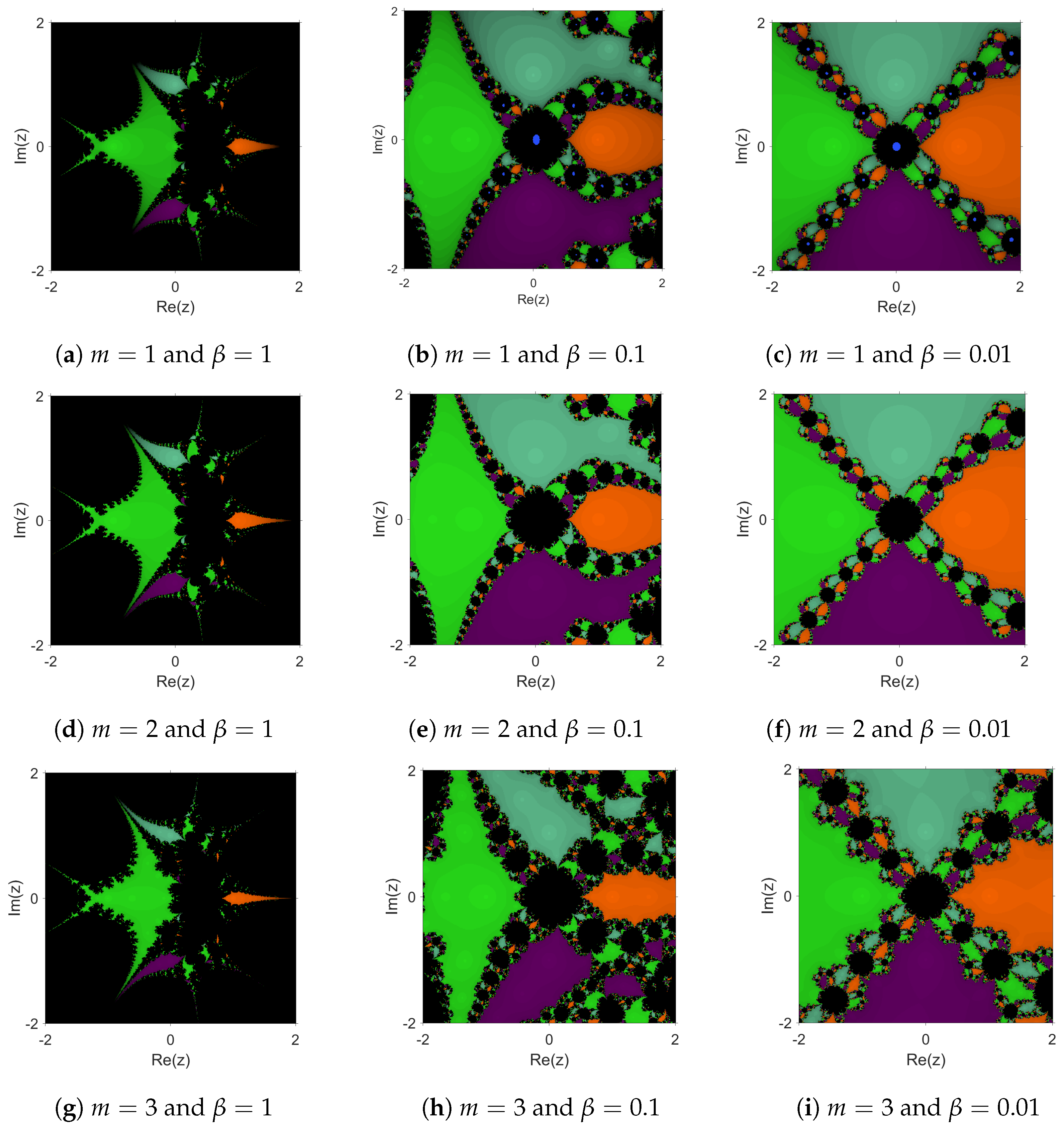
Figure 1. Dynamical planes for different m and β .
Symmetry 15 00536 g001
Table 1. Numerical results with different values of β .
β rR m ( r ) λ ( r ) b l ( r ) γ
0.01 0.2016 1.6563 0.2681 0.2970 0.1417 0.2173
0.02 0.2018 1.6461 0.2688 0.2977 0.1417 0.2177
0.03 0.2020 1.6360 0.2696 0.2984 0.1417 0.2180
0.1 0.2036 1.5686 0.2748 0.3037 0.1417 0.2202
0.2 0.2059 1.4815 0.2825 0.3114 0.1417 0.2234
0.3 0.2083 1.4035 0.2903 0.3195 0.1417 0.2267
1.0 0.2324 1.0256 0.3555 0.3899 0.1417 0.2513
1.1 0.2376 0.9877 0.3671 0.4034 0.1417 0.2553
1.2 0.2438 0.9524 0.3800 0.4185 0.1417 0.2595
Disclaimer/Publisher’s Note: The statements, opinions and data contained in all publications are solely those of the individual author(s) and contributor(s) and not of MDPI and/or the editor(s). MDPI and/or the editor(s) disclaim responsibility for any injury to people or property resulting from any ideas, methods, instructions or products referred to in the content.