
Exact Solutions for the Generalized Atangana-Baleanu-Riemann Fractional (3 + 1)-Dimensional Kadomtsev–Petviashvili Equation


1
Faculty of Mathematical Physics, Nanjing Institute of Technology, Nanjing 211167, China
2
Faculty of Electric Power Engineering, Nanjing Institute of Technology, Nanjing 211167, China
*
Author to whom correspondence should be addressed.
Symmetry 2023, 15(1), 3; https://doi.org/10.3390/sym15010003
Submission received: 9 November 2022
/
Revised: 13 December 2022
/
Accepted: 17 December 2022
/
Published: 20 December 2022
(This article belongs to the Special Issue Recent Advances in Symmetries Methods and Other Approaches to Nonlinear Differential Equations)
Abstract
:In this article, the generalized Jacobi elliptic function expansion method with four new Jacobi elliptic functions was used to the generalized fractional (3 + 1)-dimensional Kadomtsev–Petviashvili (GFKP) equation with the Atangana-Baleanu-Riemann fractional derivative, and abundant new types of analytical solutions to the GFKP were obtained. It is well known that there is a tight connection between symmetry and travelling wave solutions. Most of the existing techniques to handle the PDEs for finding the exact solitary wave solutions are, in essence, a case of symmetry reduction, including nonclassical symmetry and Lie symmetries etc. Some 3D plots, 2D plots, and contour plots of these solutions were simulated to reveal the inner structure of the equation, which showed that the efficient method is sufficient to seek exact solutions of the nonlinear partial differential models arising in mathematical physics.
1. Introduction
In more recent years, the fractional calculus and fractional nonlinear partial differential equations (FNPDE) have played an important role in the investigation nonlinear phenomena. Many scientists in the world are absorbed by this topic, and searching for the exact solutions of these FNPDES is significant in the study of nonlinear phenomena, including the nonlinear wave observed in mechanics [1], ecological and economic systems [2], two-scale thermal science [3], optical fibers [4], chaotic oscillations [5], atmospheric science [6], telegraph transmission [7], etc. [8,9,10,11]. To date, many powerful methods have been proposed for this subject, such as the Bäcklund transformation method [12], Darboux transformation [13], Hirota bilinear method [14], improved F-expansion method [15], sine-Gordon method [16], projective Riccati equations method [17], G’/G-expansion method [18], (G’/G,1/G)-expansion method [19], improved (m + G’/G)-expansion method [20], improved G’/G2-expansion method [21], the first integral method [22], Generalized Exp-Function Method [23], Exp(−φ(ξ))-Expansion Method [24], and Lie symmetry method, which are connected to the wave transformations of equations that do not change the set of solutions [25], among others [26,27,28,29,30,31,32,33,34,35,36].
Since calculus was founded by Newton and Leibniz in the 1660s, the fractional calculus has been gradually studied by many scholars all over the world. To date, there have been many definitions of the fractional derivative. The most classic definitions are the Riemann–Liouville fractional derivative [37], Caputo fractional derivative [38], Jumaries’s fractional derivative [39], Ji-Huan He’s fractional derivative [40], Atangana’s fractional derivative [41], M-fractional derivative [42], conformable fractional derivative [43], Atangana–Baleanu–Caputo Operator [44], and the Atangana-Baleanu-Riemann derivative [45,46,47,48,49,50,51]. Each definition has its own advantages and limitations. Compared with other definitions, the ABR derivative is more convenient for integration operations due to the introduction of series and rational standardized functions.
Consider the following generalized Atangana-Baleanu-Riemann time-fractional (3 + 1)-dimensional Kadomtsev-Petviashvili (KP) equation [52,53,54,55,56,57,58]:
where are real numbers. The wave function means the Atangana-Baleanu-Riemann (ABR) fractional derivative [45,46,47,48,49,50,51]; when , the lump solitons of Equation (1) were deduced using Hirota’s bilinear transformation method in Ref. [52]. The solutions of many other deformed forms of (3 + 1)-dimensional KP equation can be found in Refs. [53,54,55,56,57,58,59]. In this paper, we extended the Jacobi elliptic function expansion method [60,61] to Equation (1) utilizing a wave transformation.
The ABR fractional derivative is defined as follows.
Definition 1.
Theorem 1.
The relation between the ABR fractional derivative and Riemann-Liouville integral operator is given by
Proof.
where is a Riemann–Liouville integral operator. □
The rest of the paper is organized as follows. In Section 2, we introduce the generalized Jacobi elliptic function expansion method, while in Section 3, some exact solutions of the GFKP equation are found and discussed utilizing the proposed methods. Finally, the conclusion is presented in Section 4.
2. Summary of the Generalized Jacobi Elliptic Functions Expansion Method
Consider the following (3 + 1)-dimensional ABR fractional differential equation:
We use the following wave transformation:
where constant means the wave speed to be determined later.
For we have
.
Thus, Equation (2) reduces to an ordinary differential equation:
Assume that Equation (5) has the following solution:
where are constants to be determined later. are arbitrary functions with the variables and t. The parameter can be determined by balancing the highest-order derivative terms with the nonlinear terms in Equation (2). is an arbitrary array of the four functions and , which are expressed as follows [60,61]:
where are arbitrary constants. The functions satisfy the restricted relations (4) and (5a–5d) mentioned in [60,61]. Using the standard steps [60,61], we can construct some new solutions of Equations (2) and (5).
3. Exact Solutions to the Fractional (3 + 1)-Dimensional KP Equation
Substituting Equation (3) into Equation (1), we obtain:
By balancing the highest-order linear term and the nonlinear term in Equation (8), we can obtain . Thus, we assume that Equation (8) has the following solutions:
where .
Substituting (4) and (5a–5d) mentioned in [60,61] separately along with Equation (9) into Equation (8) and setting the coefficients of , to zero yields ODEs with respect to the unknowns . After solving the ODEs by mathematical software and Wu elimination, we could determine the following solutions.
Set 1. When
Case 1
Case 2
Case 3
Case 4
Case 5
Case 6
Case 7
Case 8
Case 9
Case 10
Case 11
Case 12
where unmentioned are equal to zero, as are the following situations. According to Equations (3), (7) and (9) and case 1–case 12, we can deduce the following solutions of Equation (1):
where
The expression of has the similar forms in the following situations.
Some simulations of are shown in Figure 1, Figure 2, Figure 3 and Figure 4. The corresponding parameter values were selected as follows:
With the same process, we can derive the other three families of new exact solutions of Equation (1) as follows.
Set 2. When
Case 13
Case 14
Case 15
Case 16
Case 17
Case 18
Case 19
Case 20
Case 21
Case 22
We obtain the following solutions of Equation (1):
Set 3. When
Case 23
Case 24
Case 25
Case 26
Case 27
Case 28
Case 29
We obtain the following solutions of Equation (1):
Set 4. When
Case 30
Case 31
We obtain the following solutions of Equation (1):
In the above cases, we have:
Notice that the Jacobian elliptic functions have the following degenerative properties. Setting the modulus yields , , and when , it derives that and . We can obtain some solitary wave solutions and trigonometric function wave solutions.
Remark. Solutions are degenerated to solitary solutions when the modulus , and solutions are degenerated to triangular functions solutions when the modulus .
4. Results and Discussion
After utilizing the generalized Jacobi elliptic functions expansion method, we obtained many types of exact explicit solutions as in Equation (1); some structure of these solutions are simulated in Figure 1, Figure 2, Figure 3, Figure 4, Figure 5, Figure 6, Figure 7, Figure 8, Figure 9, Figure 10, Figure 11 and Figure 12. The visualization can help us better understanding the dynamic behavior and propagation property of these solutions. For example, the Jacobi function wave solution of Equation (1) is shown in Figure 1. From the solution, we can find that the waveform changes periodically in the upper and lower planes, while the double periodic solution makes cyclical changes upward, as shown in Figure 2. In Figure 3 and Figure 4, the waveform widths of and in the upper and lower directions show periodic changes in alternating size. The famous Jacobi oval cosine wave solution and bell-shape soliton solution are plotted in Figure 5 and Figure 6. The simulations of various other different forms of double periodic wave solutions are shown in Figure 7, Figure 8, Figure 9, Figure 10 and Figure 11. From Figure 10, we can find that there are two parallel asymptotes between the adjacent two cycles of the wave function. Each set of waves was suppressed in a region of equal width. When , we can find that the 3D plot of on the dimension is different from the dimension, which is shown in Figure 12. If we select different values for the parameters and , the shape and position of Jacobi function solutions produces an offset, which is simulated in Figure 13. These different propagation patterns may explain the different phenomena for this model.
5. Conclusions
In this paper, we succeeded to propose the generalized Jacobi elliptic function expansion method for finding new exact solutions of nonlinear evolution equations by constructing the four new types of Jacobian elliptic functions (4). Using this method and computerized symbolic computation, we found 31 types of exact solutions for the generalized fractional (3 + 1)-dimensional KP equation, including Jacobi elliptic functions solutions, bell-shape soliton solution, solitary wave solutions, trigonometric function solutions, and periodic wave solutions in the mixed form to the GFKP. More importantly, our method is a simple and powerful technique to find new solutions to various kinds of nonlinear evolution equations. We believe that this method should play an important role in finding exact solutions in mathematical physics.
Author Contributions
B.H. and J.W. have contributed equally to this work. All authors have read and agreed to the published version of the manuscript.
Funding
This work is supported by the practical innovation training program projects for the university students of Jiangsu Province (Grant No. 202211276054Y), Natural science research projects of Institutions in Jiangsu Province (Grant No. 18KJB110013) and Nanjing Institute of Technology (Grant No. ZKJ201513).
Institutional Review Board Statement
Not applicable.
Informed Consent Statement
Not applicable.
Data Availability Statement
The authors affirm the availability of data and material in deriving the solutions mentioned in this manuscript.
Acknowledgments
The authors would like to thank the editors and reviewers for their help and useful suggestions.
Conflicts of Interest
The authors declare no conflict of interest. The funders had no role in the design of the study; in the collection, analyses, or interpretation of data; in the writing of the manuscript; or in the decision to publish the results.
References
- Zhang, R.F.; Bilige, S. Bilinear neural network method to obtain the exact analytical solutions of nonlinear partial differential equations and its application to p-gBKP equation. Nonlinear Dyn. 2019, 95, 3041–3048. [Google Scholar] [CrossRef]
- Almutairi, A.; El-Metwally, H.; Sohaly, M.A.; Elbaz, I.M. Lyapunov stability analysis for nonlinear delay systems under random effects and stochastic perturbations with applications in finance and ecology. Adv. Differ. Equ. 2021, 2021, 186. [Google Scholar] [CrossRef]
- He, J.H. Seeing with a single scale is always unbelieving: From magic to two-scale fractal. Therm. Sci. 2021, 25, 1217–1219. [Google Scholar] [CrossRef]
- Yokus, A.; Baskonus, H.M. Dynamics of traveling wave solutions arising in fiber optic communication of some nonlinear models. Soft Comput. 2022, 26, 13605–13614. [Google Scholar] [CrossRef]
- Tavazoei, M.S.; Haeri, M.; Jafari, S.; Bolouki, S.; Siami, M. Some applications of fractional calculus in suppression of chaotic oscillations. IEEE Trans. Ind. Electron. 2008, 55, 4094–4101. [Google Scholar] [CrossRef]
- Korn, P. A Regularity-Aware algorithm for variational data assimilation of an idealized coupled Atmosphere-Ocean Model. J. Sci. Comput. 2018, 79, 748–786. [Google Scholar] [CrossRef] [Green Version]
- Radu, C.C.; Eugene, C.E.; Cicero, L.F.; Jerome, A.G. Fractional telegraph equations. J. Math. Anal. Appl. 2002, 276, 145–159. [Google Scholar]
- Abdelwahed, H.G.; El-Shewy, E.K.; Abdelrahman, M.A.; Alsarhana, A.F. On the physical nonlinear (n + 1)-dimensional Schrödinger equation applications. Results Phys. 2021, 21, 103798. [Google Scholar] [CrossRef]
- Samei, M.E.; Karimi, L.; Kaabar, M.K.A. To investigate a class of multi-singular pointwise defined fractional q–integro-differential equation with applications. AIMS Math. 2022, 7, 7781–7816. [Google Scholar] [CrossRef]
- Yousef, F.; Alquran, M.; Jaradat, I.; Momani, S.; Baleanu, D. New Fractional Analytical Study of Three-Dimensional Evolution Equation Equipped With Three Memory Indices. J. Comput. Nonlinear Dyn. 2019, 14, 111008. [Google Scholar] [CrossRef]
- Yousef, F.; Alquran, M.; Jaradat, I.; Momani, S.; Baleanu, D. Ternary-fractional differential transform schema: Theory and application. Adv. Differ. Equ. 2019, 2019, 197. [Google Scholar] [CrossRef]
- Lu, D.C.; Hong, B.J. Bäcklund transformation and n-soliton-like solutions to the combined KdV-Burgers equation with variable coefficients. Int. J. Nonlinear Sci. 2006, 1, 3–10. [Google Scholar]
- Matveev, V.A.; Salle, M.A. Darboux Transformations and Solitons; Springer: Berlin/Heidelberg, Germany, 1991. [Google Scholar]
- Hu, X.B.; Ma, W.X. Application of Hirotas bilinear formalism to the Toeplitz lattice-some special soliton-like solutions. Phys. Lett. A 2002, 293, 161–165. [Google Scholar] [CrossRef]
- Bashar, M.H.; Islam, S.M.R. Exact solutions to the (2 + 1)-Dimensional Heisenberg ferromagnetic spin chain equation by using modified simple equation and improve F-expansion methods. Phys. Open 2020, 5, 100027. [Google Scholar] [CrossRef]
- Kundu, P.R.; Fahim MR, A.; Islam, M.E.; Akbar, M.A. The sine-Gordon expansion method for higher-dimensional NLEEs and parametric analysis. Heliyon 2021, 7, e06459. [Google Scholar] [CrossRef] [PubMed]
- Lu, D.C.; Hong, B.J.; Tian, L.X. New explicit exact solutions for the generalized coupled Hirota-Satsuma KdV system. Comput. Math. Appl. 2007, 53, 1181–1190. [Google Scholar] [CrossRef] [Green Version]
- Mohanty, S.K.; Kravchenko, O.V.; Dev, A.N. Exact traveling wave solutions of the Schamel Burgers equation by using generalized-improved and generalized (G’/G) expansion methods. Results Phys. 2022, 33, 105124. [Google Scholar] [CrossRef]
- Siddique, I.; Jaradat, M.M.; Zafar, A.; Mehdi, K.B.; Osman, M.S. Exact traveling wave solutions for two prolific conformable M-Fractional differential equations via three diverse approaches. Results Phys. 2021, 33, 105216. [Google Scholar] [CrossRef]
- Ismael, H.F.; Bulut, H.; Baskonus, H.M. Optical soliton solutions to the Fokas–Lenells equation via sine-Gordon expansion method and (m + (G’/G))-expansion method. Pramana 2020, 94, 35. [Google Scholar] [CrossRef]
- Mohyud-Din, S.T.; Bibi, S. Exact solutions for nonlinear fractional differential equations using G′/G2-expansion method. Alex. Eng. J. 2018, 57, 1003–1008. [Google Scholar] [CrossRef]
- Ma, W.-X.; Osman, M.; Arshed, S.; Raza, N.; Srivastava, H. Practical analytical approaches for finding novel optical solitons in the single-mode fibers. Chin. J. Phys. 2021, 72, 475–486. [Google Scholar] [CrossRef]
- Shakeel, M.; Attaullah; Alaoui, M.K.; Zidan, A.M.; Shah, N.A.; Weera, W. Closed-Form solutions in a Magneto-Electro-Elastic circular rod via generalized Exp-function method. Mathematics 2022, 10, 3400. [Google Scholar] [CrossRef]
- Rani, A.; Shakeel, M.; Kbiri Alaoui, M.; Zidan, A.M.; Shah, N.A.; Junsawang, P. Application of the Exp(−φ(ξ))-expansion method to find the soliton solutions in biomembranes and nerves. Mathematics 2022, 10, 3372. [Google Scholar] [CrossRef]
- Nass, A.M. Lie symmetry analysis and exact solutions of fractional ordinary differential equations with neutral delay. Appl. Math. Comput. 2019, 347, 370–380. [Google Scholar] [CrossRef]
- Yue, C.; Lu, D.; Khater, M.M.A.; Abdel-Aty, A.-H.; Alharbi, W.; Attia, R.A.M. On explicit wave solutions of the fractional nonlinear DSW system via the modified Khater method. Fractals 2020, 28, 2040034. [Google Scholar] [CrossRef]
- He, J.H.; Elagan, S.K.; Li, Z.B. Geometrical explanation of the fractional complex transform and derivative chain rule for fractional calculus. Phys. Lett. A 2012, 376, 257–259. [Google Scholar] [CrossRef]
- He, J.H. Fractal calculus and its geometrical explanation. Results Phys. 2018, 10, 272–276. [Google Scholar] [CrossRef]
- Ghanbari, B.; Inc, M.; Yusuf, A.; Baleanu, D.; Bayram, M. Families of exact solutions of Biswas-Milovic equation by an exponential rational function method. Tbil. Math. J. 2020, 13, 39–65. [Google Scholar] [CrossRef]
- Hong, B.J. Exact solutions for the conformable fractional coupled nonlinear Schrödinger equations with variable coefficients. J. Low Freq. Noise Vib. Act. Control 2022, 41, 1–14. [Google Scholar] [CrossRef]
- Yu, F.; Yu, Q.; Chen, H.; Kong, X.; Mokbel, A.A.M.; Cai, S.; Du, S. Dynamic analysis and audio encryption application in IoT of a multi-scroll fractional-order hopfield neural network. Fractal Fract. 2022, 6, 370. [Google Scholar] [CrossRef]
- Hong, B.J.; Lu, D.C.; Chen, W. Exact and approximate solutions for the fractional Schrödinger equation with variable coefficients. Adv. Differ. Equ. 2019, 2019, 370. [Google Scholar] [CrossRef]
- Shah, N.A.; Agarwal, P.; Chung, J.D.; El-Zahar, E.R.; Hamed, Y.S. Analysis of Optical Solitons for Nonlinear Schrödinger Equation with Detuning Term by Iterative Transform Method. Symmetry 2020, 12, 1850. [Google Scholar] [CrossRef]
- Alquran, M.; Yousef, F.; Alquran, F.; Sulaiman, T.A.; Yusuf, A. Dual-wave solutions for the quadratic–cubic conformable-Caputo time-fractional Klein–Fock–Gordon equation. Math. Comput. Simul. 2021, 185, 62–76. [Google Scholar] [CrossRef]
- Singh, J.; Secer, A.; Swroop, R.; Kumar, D. A reliable analytical approach for a fractional model of advection-dispersion equation. Nonlinear Eng. 2019, 8, 107–116. [Google Scholar] [CrossRef]
- Shah, N.A.; Hamed, Y.S.; Abualnaja, K.M.; Chung, J.-D.; Shah, R.; Khan, A. A Comparative Analysis of Fractional-Order Kaup–Kupershmidt Equation within Different Operators. Symmetry 2022, 14, 986. [Google Scholar] [CrossRef]
- Haq, A. Partial-approximate controllability of semi-linear systems involving two Riemann-Liouville fractional derivatives. Chaos Solitons Fractals 2022, 157, 111923. [Google Scholar] [CrossRef]
- Caputo, M. Linear models of dissipation whose Q is almost frequency independent: Part II. Geophys. J. Int. 1967, 13, 529–539. [Google Scholar] [CrossRef]
- Guner, O.; Atik, H.; Kayyrzhanovich, A.A. New exact solution for space-time fractional differential equations via (G’/G)-expansion method. Optik 2017, 130, 696–701. [Google Scholar] [CrossRef]
- He, J.H. A tutorial review on fractal spacetime and fractional calculus. Int. J. Theor. Phys. 2014, 53, 3698–3718. [Google Scholar] [CrossRef]
- Atangana, A.; Baleanu, D.; Alsaedi, A. Analysis of time-fractional Hunter-Saxton equation: A model of neumatic liquid crystal. Open Phys. 2016, 14, 145–149. [Google Scholar] [CrossRef]
- Yao, S.-W.; Manzoor, R.; Zafar, A.; Inc, M.; Abbagari, S.; Houwe, A. Exact soliton solutions to the Cahn-Allen equation and Predator-Prey model with truncated M-fractional derivative. Results Phys. 2022, 37, 105455. [Google Scholar] [CrossRef]
- Khalil, R.; Horani, M.A.; Yousef, A.; Sababheh, M. A new definition of fractional derivative. J. Comput. Appl. Math. 2014, 264, 65–70. [Google Scholar] [CrossRef]
- Shah, N.A.; Alyousef, H.A.; El-Tantawy, S.A.; Shah, R.; Chung, J.D. Analytical investigation of Fractional-Order Korteweg–De-Vries-Type equations under Atangana–Baleanu–Caputo operator: Modeling Nonlinear Waves in a Plasma and Fluid. Symmetry 2022, 14, 739. [Google Scholar] [CrossRef]
- Atangana, A.; Koca, I. Chaos in a simple nonlinear system with Atangana-Baleanu derivatives with fractional order. Chaos Solitons Fractals 2016, 89, 447–454. [Google Scholar] [CrossRef]
- Hashemi, M.S. A novel approach to find exact solutions of fractional evolution equations with non-singular kernel derivative. Chaos Solitons Fractals 2021, 152, 111367. [Google Scholar] [CrossRef]
- Tajadodi, H. A Numerical approach of fractional advection-diffusion equation with Atangana-Baleanu derivative. Chaos Solitons Fractals 2020, 130, 109527. [Google Scholar] [CrossRef]
- Yusuf, A.; Inc, M.; Aliyu, A.I.; Baleanu, D. Optical solitons possessing beta derivative of the Chen-Lee-Liu equation in optical fibers. Front. Phys. 2019, 7, 00034. [Google Scholar] [CrossRef] [Green Version]
- Khater, M.M.A.; Ghanbari, B.; Nisar, K.S.; Kumar, D. Novel exact solutions of the fractional Bogoyavlensky–Konopelchenko equation involving the Atangana-Baleanu-Riemann derivative. Alex. Eng. J. 2020, 59, 2957–2967. [Google Scholar] [CrossRef]
- Shafiq, M.; Abbas, M.; Abdullah, F.A.; Majeed, A.; Abdeljawad, T.; Alqudah, M.A. Numerical solutions of time fractional Burgers’ equation involving Atangana-Baleanu derivative via cubic B-spline functions. Results Phys. 2022, 34, 105244. [Google Scholar] [CrossRef]
- Sarwar, S. New Rational Solutions of fractional-order Sharma-Tasso-Olever equation with Atangana-Baleanu derivative arising in physical sciences. Results Phys. 2020, 19, 103621. [Google Scholar] [CrossRef]
- Elboree, M.K. Lump solitons, rogue wave solutions and lump-stripe interaction phenomena to an extended (3 + 1)-dimensional KP equation. Chin. J. Phys. 2020, 63, 290–303. [Google Scholar] [CrossRef]
- Mohammed, K. New exact traveling wave solutions of the (3 + 1)-dimensional Kadomtsev-Petviashvili (KP) equation. Commun. Nonlinear Sci. Numer. Simul. 2009, 14, 1169–1175. [Google Scholar]
- Ma, W.X.; Zhu, Z.N. Solving the (3 + 1)-dimensional generalized KP and BKP equations by the multiple exp-function algorithm. Appl. Math. Comput. 2012, 218, 11871–11879. [Google Scholar] [CrossRef]
- Hussain, A.; Anjum, A.; Junaid-U-Rehman, M.; Khan, I.; Sameh, M.A.; Al-Johani, A.S. Symmetries, optimal system, exact and soliton solutions of (3 + 1)-dimensional Gardner-KP equation. J. Ocean. Eng. Sci. 2022; in press. [Google Scholar] [CrossRef]
- Hao, X.Z.; Liu, Y.P.; Li, Z.B.; Ma, W.X. Painlevé analysis, soliton solutions and lump-type solutions of the (3 + 1)-dimensional generalized KP equation. Comput. Math. Appl. 2019, 77, 724–730. [Google Scholar] [CrossRef]
- Wazwaz, A.M. Multiple-soliton solutions for a (3 + 1)-dimensional generalized KP equation. Commun. Nonlinear Sci. Numer. Simul. 2012, 17, 491–495. [Google Scholar] [CrossRef]
- Elboree, M.K. Soliton molecules and exp(−Φ(ζ)) expansion method for the new (3 + 1)-dimensional kadomtsev-Petviashvili (KP) equation. Chin. J. Phys. 2021, 71, 623–633. [Google Scholar] [CrossRef]
- Wazwaz, A.M.; El-Tantawy, S.A. A new (3 + 1)-dimensional generalized Kadomtsev–Petviashvili equation. Nonlinear Dyn. 2016, 84, 1107–1112. [Google Scholar] [CrossRef]
- Hong, B.J. New Jacobi elliptic functions solutions for the variable-coeffiffifficient mKdV equation. Appl. Math. Comput. 2009, 215, 2908–2913. [Google Scholar]
- Hong, B.J. New exact Jacobi elliptic functions solutions for the generalized coupled Hirota-Satsuma KdV system. Appl. Math. Comput. 2010, 217, 472–479. [Google Scholar] [CrossRef]
Figure 1.
The 3D plot, 2D plot, and contour plot of with .
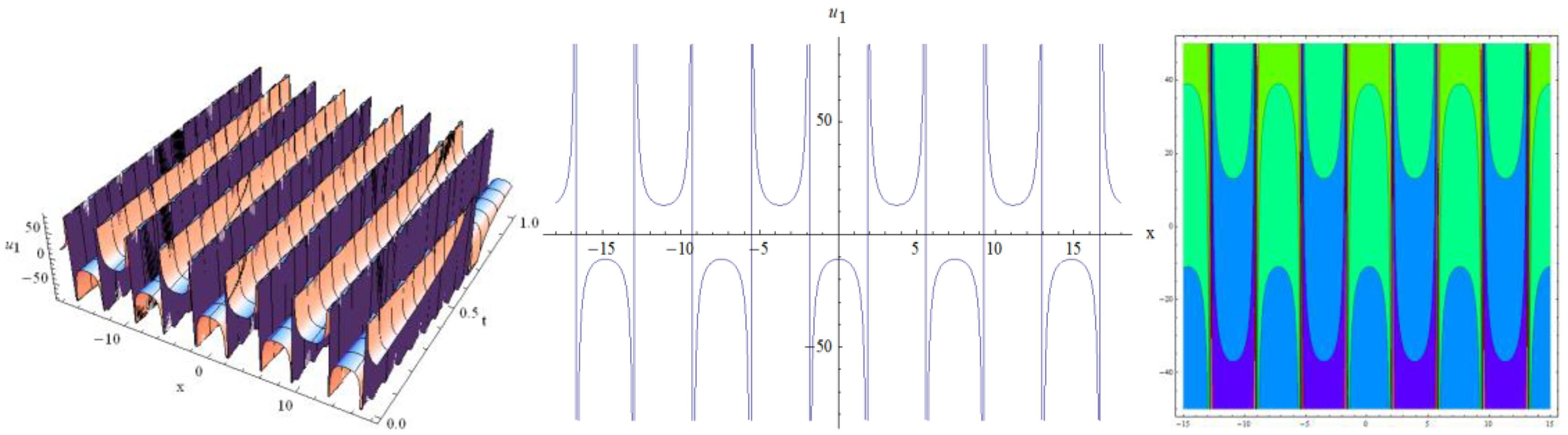
Figure 2.
The 3D plot, 2D plot, and contour plot of with .

Figure 3.
The 3D plot, 2D plot, and contour plot of with .
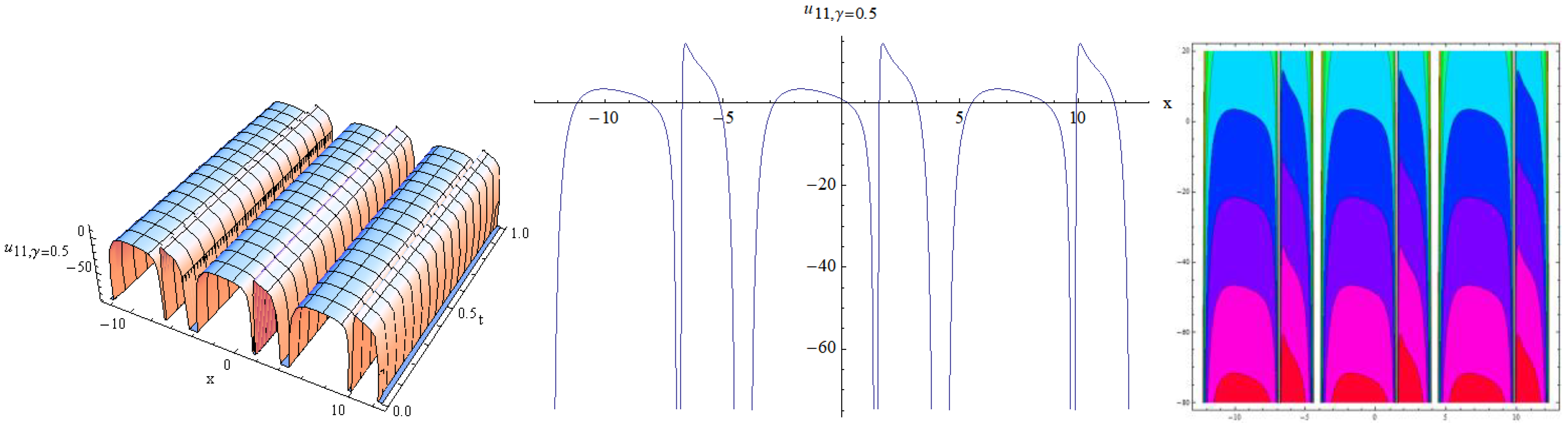
Figure 4.
The 3D plot, 2D plot, and contour plot of with .
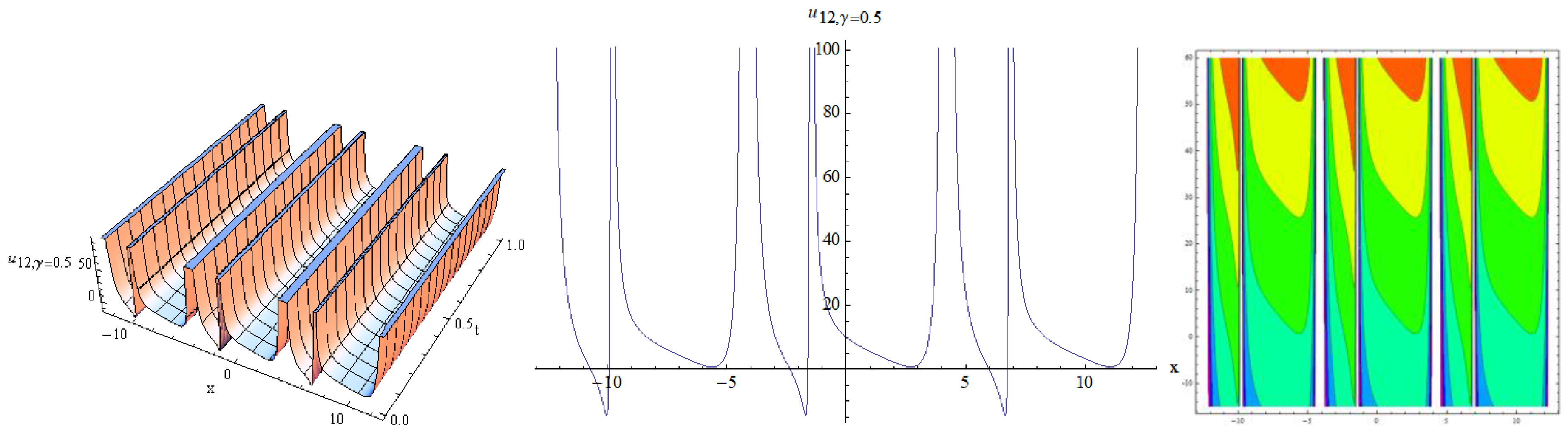
Figure 5.
The 3D plot, 2D plot, and contour plot of with .
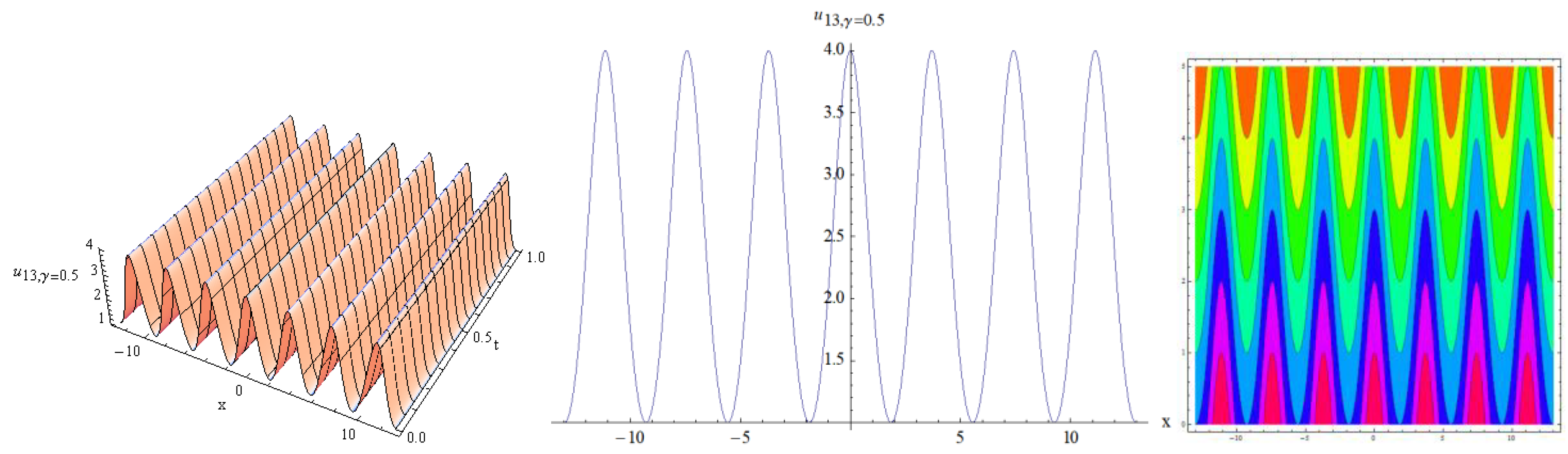
Figure 6.
The 3D plot, 2D plot, and contour plot of bell-shape soliton with .
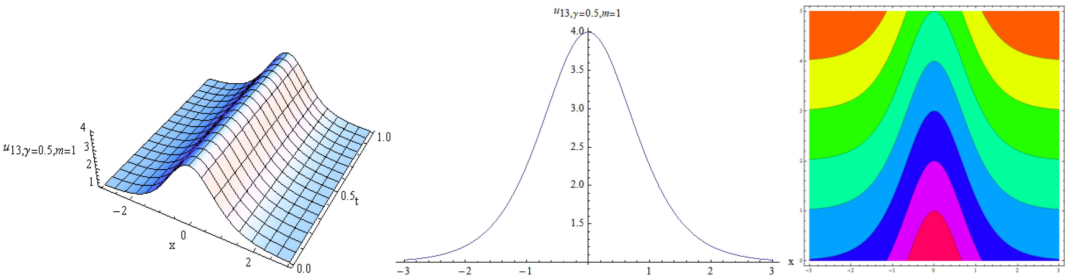
Figure 7.
The 3D plot, 2D plot, and contour plot of with .
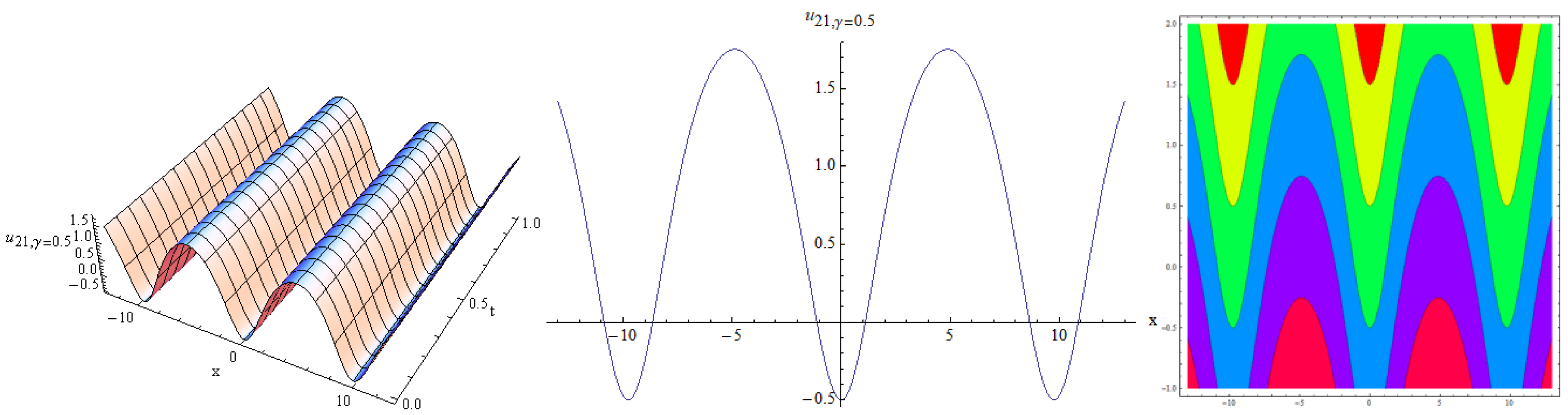
Figure 8.
The 3D plot, 2D plot, and contour plot of with .

Figure 9.
The 3D plot, 2D plot, and contour plot of with .

Figure 10.
The 3D plot, 2D plot, and contour plot of with .
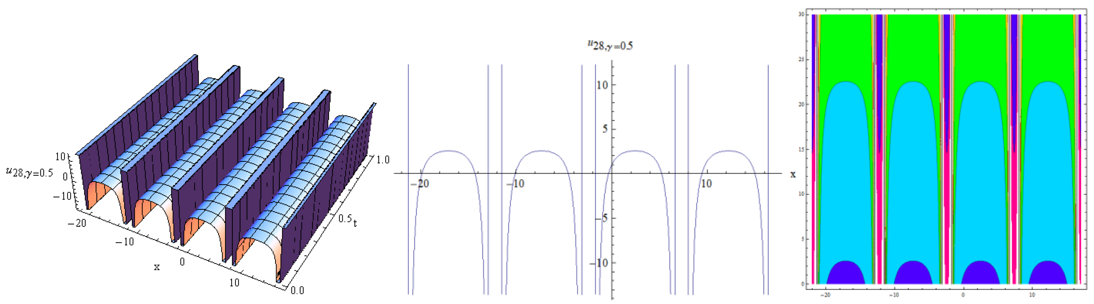
Figure 11.
The 3D plot, 2D plot, and contour plot of with .

Figure 12.
The 3D plot, 2D plot, and contour plot of with .
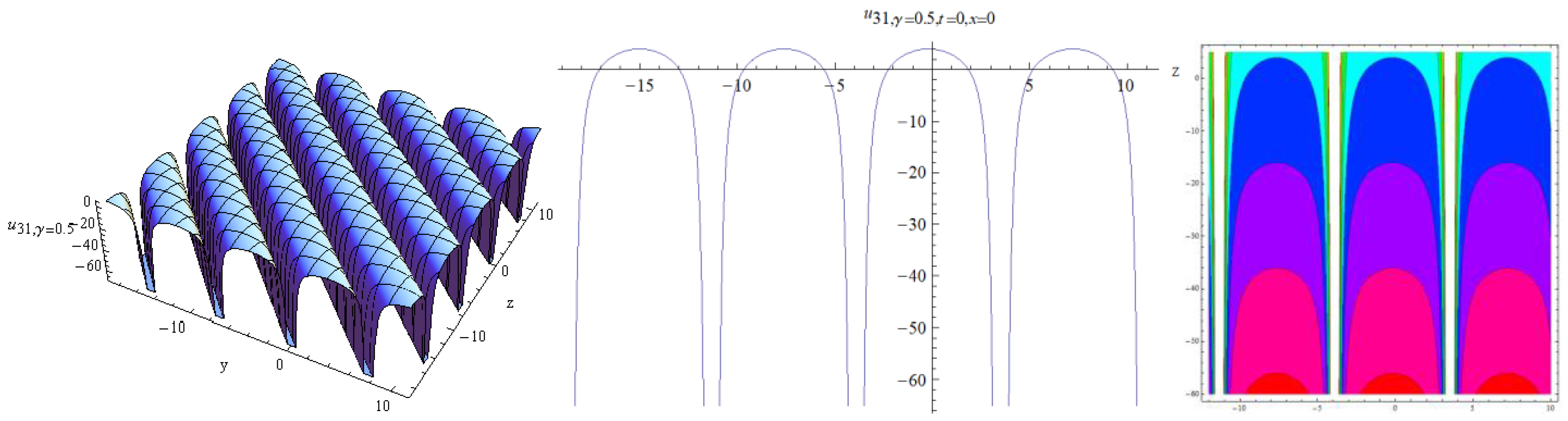
Figure 13.
The changes in waveform of with different values of and .

Disclaimer/Publisher’s Note: The statements, opinions and data contained in all publications are solely those of the individual author(s) and contributor(s) and not of MDPI and/or the editor(s). MDPI and/or the editor(s) disclaim responsibility for any injury to people or property resulting from any ideas, methods, instructions or products referred to in the content. |
© 2022 by the authors. Licensee MDPI, Basel, Switzerland. This article is an open access article distributed under the terms and conditions of the Creative Commons Attribution (CC BY) license (https://creativecommons.org/licenses/by/4.0/).
Share and Cite
MDPI and ACS Style
Hong, B.; Wang, J. Exact Solutions for the Generalized Atangana-Baleanu-Riemann Fractional (3 + 1)-Dimensional Kadomtsev–Petviashvili Equation. Symmetry 2023, 15, 3. https://doi.org/10.3390/sym15010003
AMA Style
Hong B, Wang J. Exact Solutions for the Generalized Atangana-Baleanu-Riemann Fractional (3 + 1)-Dimensional Kadomtsev–Petviashvili Equation. Symmetry. 2023; 15(1):3. https://doi.org/10.3390/sym15010003
Chicago/Turabian StyleHong, Baojian, and Jinghan Wang. 2023. "Exact Solutions for the Generalized Atangana-Baleanu-Riemann Fractional (3 + 1)-Dimensional Kadomtsev–Petviashvili Equation" Symmetry 15, no. 1: 3. https://doi.org/10.3390/sym15010003
Note that from the first issue of 2016, this journal uses article numbers instead of page numbers. See further details here.