New Analytical Solutions for Coupled Stochastic Korteweg–de Vries Equations via Generalized Derivatives

Abstract

In this paper, the coupled nonlinear KdV (CNKdV) equations are solved in a stochastic environment. Hermite transforms, generalized conformable derivative, and an algorithm that merges the white noise instruments and the $({\mathfrak{G}}^{\prime }/{\mathfrak{G}}^{\mathfrak{2}})$-expansion technique are utilized to obtain white noise functional conformable solutions for these equations. New stochastic kinds of periodic and soliton solutions for these equations under conformable generalized derivatives are produced. Moreover, three-dimensional (3D) depictions are shown to illustrate that the monotonicity and symmetry of the obtained solutions can be controlled by giving a value of the conformable parameter. Furthermore, some remarks are presented to give a comparison between the obtained wave solutions and the wave solutions constructed under the conformable derivatives and Newton’s derivatives.

1. Introduction

Nonlinear phenomena exist in numerous areas of natural sciences, such as applied mathematics and physics, computational fluid dynamics, and some other sciences [1]. These phenomena can be represented by nonlinear partial differential equations (PDEs) [2,3,4,5]. The importance of the field of nonlinear differential equations lies in the search for their exact solutions that in turn give an explanation for multiple phenomena. There is a significant class of nonlinear differential equations known as fractional differential equations, and there have been many studies and advancements, particularly in determining their exact solutions. Some models of differential equations contain random variables, called stochastic differential equations (SDEs) and deterministic differential equations (DDEs). Because of the fact that the random kinds are more natural than deterministic kinds, we confine our task to stochastic PDEs with recently generalized derivatives.

The concept of generalized derivatives or fractional derivatives is to extend traditional derivatives such as Newton’s classical derivative [6,7,8]. Recently, Khalil et al. [9] gave a simple concept of fractional derivatives called conformable derivatives, which depend on the basic limit notion. Consequently, certain generalizations have been obtained in the literature such as the definitions of Zhao and Luo [10,11] and Hyder and Soliman [12].

The KdV equation is a world-class mathematical model for the characterization of long nonlinear weakly wave diffusion in scattered media. It has many applications in physics, among them: gravity waves in shallow water [13], bubbly fluid waves [14], ocean waves, and numerous others [15]. This wide range of applicability for the KdV equation is characterized by the common effect of the lowest-order, cubic, and long-wave dispersal terms. Moreover, one can obtain derivations of the KdV equation for various physical contexts [16,17,18]. In recent decades, the KdV equation has been developed and modified into the modified KdV equation (mKdV) [19], two-mode KdV equation (TKdV) [20], two-mode modified KdV equation (TmKdV) [19], coupled nonlinear KdV equations [21], the KdV equation in random environments [22], etc. All these modifications and developments of the KdV equation aimed to obtain more general solutions than their predecessors.

Given the importance of the exact solutions for SDEs and DDEs, searching for different techniques to find these solutions has become an increasingly appealing field in applied mathematics. So, new techniques are being sought to tackle more sophisticated problems. Hence, numerous new techniques have been proposed, for example, the Kudryashov technique and all of their modifications [23,24,25,26], the F-expansion technique [27], Jacobi elliptic function technique [28,29], (${\mathfrak{G}}^{\prime }/\mathfrak{G}$)-expansion technique [30], and (${\mathfrak{G}}^{\prime }/{\mathfrak{G}}^{\mathfrak{2}}$)-expansion technique [31]. Moreover, there are ongoing advancements in techniques in terms of their modifications and generalizations for obtaining solutions for SDEs and DDEs, see [32,33,34,35] and references therein.

This work is devoted to inspecting diverse deterministic and stochastic accurate solutions for the CNKdV equations under recently generalized derivatives. Foremost, we present an algorithm for solving conformable stochastic partial differential equations (SPDEs). This algorithm merges the utilizing of the white noise instruments, the generalized conformable derivative, and the $({\mathfrak{G}}^{\prime }/{\mathfrak{G}}^{\mathfrak{2}})$-expansion technique. Using the offered algorithm, we produce a family of accurate deterministic solutions for the CNKdV. Under certain restrictions and the reverse Hermite transform, we transform the solutions of the deterministic CNKdV to stochastic kinds of periodic and soliton solutions for the stochastic CNKdV equations. Moreover, 3D portrayals are displayed to point out that the monotonicity and symmetry of the obtaining solutions can be controlled by giving a value of the conformable parameter. According to the current literature, this work is a novel contribution, and the proposed technique for addressing nonlinear issues is straightforward and simple to execute. Additionally, some remarks are offered to provide a comparison between the obtained wave solutions and the wave solutions constructed under the conformable derivatives and Newton’s derivatives.

2. Preliminaries

In this section, the definitions and attributes of the generalized conformable derivative are presented.

Definition 1

([36]). If we have a nonnegative continuous function $\delta :[c,d]\to \mathbb{R}$ with $\delta \left(s\right)\ne 0$ and ${\delta }^{\prime }\left(s\right)\ne 0$ for each $s\in (c,d).$ For any function $g:[c,d]\to \mathbb{R}$, the generalized conformable derivative of order $\pi \in (0,1)$ is obtained by

$$\begin{array}{c}\hfill D_s^{\pi }g\left(s\right)=\underset{\eta \to 0}{lim}\frac{g\left(s-\delta \left(s\right)+\delta \left(s\right)exp\left({\displaystyle \frac{\eta }{{\left(\delta \left(s\right)\right)}^{\pi }{\delta }^{\prime }\left(s\right)}}\right)\right)-g\left(s\right)}{\eta },\end{array}$$

(1)

assuming the limit exists.

Definition 2

([36]). Let g be a π-differentiable function on $(a,s)$, and let ${lim}_{s\to 0}{D}_s^{\pi }g\left(s\right)$ exist. Then, $D_s^{\pi }g\left(0\right)={lim}_{s\to 0}{D}_s^{\pi }g\left(s\right)$, and the generalized conformable integral of g is given by

$$\begin{array}{c}\hfill {\mathfrak{I}}^{\pi ,a}g\left(s\right)={\int }_a^s\frac{{\delta }^{\prime }\left(u\right)g\left(u\right)}{{\left(\delta \left(u\right)\right)}^{1-\pi }}du.\end{array}$$

(2)

The following theorems outline the essential properties of the generalized conformable derivative.

Theorem 1

([36]). If we have two $\pi -$ differentiable functions h and g with $0\le \pi \le 1.$, then

(a) $D_s^{\pi }\left(C\right)=0,\mathrm{for}\mathrm{all}\mathrm{constant}\mathrm{function}h\left(s\right)=C,$

(b) $D_s^{\pi }\left(s^p\right)=\left(p{s}^{p-1}\right)\left(\frac{{\left(\delta \left(s\right)\right)}^{1-\pi }}{{\delta }^{\prime }\left(s\right)}\right),p\in \mathbb{R}.$

(c) $D_s^{\pi }(c_{1}h\left(s\right)+c_{2}g\left(s\right))=c_1{D}_s^{\pi }\left(h\left(s\right)\right)+c_2{D}_s^{\pi }\left(g\left(s\right)\right),$

(d) $D_s^{\pi }\left(hg\right)\left(s\right)=h\left(s\right)D_s^{\pi }\left(g\left(s\right)\right)+g\left(s\right)D_s^{\pi }\left(h\left(s\right)\right),$

(e) $D_s^{\pi }\left(\frac{h\left(s\right)}{g\left(s\right)}\right)=\frac{g\left(s\right)D_s^{\pi }\left(h\left(s\right)\right)-h\left(s\right)D_s^{\pi }\left(g\left(s\right)\right)}{{\left(g\left(s\right)\right)}^2},g\left(s\right)\ne 0\forall s>0,$

(f) $D_s^{\pi }\left(h\left(s\right)\right)=\left(\frac{dh\left(s\right)}{ds}\right)\left(\frac{{\left(\delta \left(s\right)\right)}^{1-\pi }}{{\delta }^{\prime }\left(s\right)}\right)$.

Theorem 2

([36]). For $s>0$, suppose that h is a π-differentiable function, and suppose that g is a differentiable function its domain equal to the range of h, and its range is $\mathbb{R}$. Then, $h\left(g\right(s\left)\right)$ is π-differentiable function, and

$$\begin{array}{c}\hfill D_s^{\pi }\left(h\left(g\left(s\right)\right)\right)=\left(\frac{dh}{dg}\right)\left(\frac{dg}{ds}\right)\left(\frac{{\left(\delta \left(s\right)\right)}^{1-\pi }}{{\delta }^{\prime }\left(s\right)}\right).\end{array}$$

(3)

3. An Algorithm for Solving Conformable SPDEs

This section elucidates an algorithm for obtaining accurate wave solutions for conformable SPDEs under conformable generalized derivatives. This algorithm merges the white noise instruments, the features of conformable generalized derivatives, and the (${\mathfrak{G}}^{\prime }/{\mathfrak{G}}^{\mathfrak{2}}$)-expansion technique.

We assume the stochastic space of Kondratiev ${\left(Z\right)}_{-1}^m$ having the orthogonal basis ${\left\{Q_{\rho }\right\}}_{\rho \in P},$ such that $P=\left\{\rho =({\rho }_1,{\rho }_2,{\rho }_3,\dots );{\rho }_i\in \mathbb{N}\mathit{and}{\sum }_{i=1}^{\infty }{\rho }_i<\infty \right\}.$ We choose two elements $U,V\in {\left(Z\right)}_{-1}^m$; then, $U={\sum }_{\rho }{\vartheta }_{\rho }{Q}_{\rho }$ and $V={\sum }_{\rho }{\varpi }_{\rho }{Q}_{\rho },$ where ${\vartheta }_{\rho },{\varpi }_{\rho }\in {\mathbb{R}}^n.$ We define the wick multiplication of U and V by:

$$\begin{array}{c}\hfill U\diamond V=\sum _{\rho ,\overline{\rho }}\sum _{j=1}^m{\vartheta }_{\rho }^j{\varpi }_{\overline{\rho }}^j{Q}_{\rho +\overline{\rho }}.\end{array}$$

(4)

In addition, the U’s Hermite transform has the ability to expand by

$$\begin{array}{c}\hfill \mathcal{H}\left(U\right)=\tilde{U}\left(\tau \right)=\sum _{\rho }{\vartheta }_{\rho }{\tau }^{\rho }\in {\mathbb{C}}^m,\end{array}$$

(5)

where $\tau ={\left({\tau }_j\right)}_{j\ge 1}\in {\mathbb{C}}^{\mathbb{N}}$ and ${\tau }^{\rho }={\Pi }_{j=1}^{\infty }{\tau }^{{\rho }_j}$. Equations (4) and (5) can be used to derive the relationship between Wick multiplication and Hermite transform as the following:

$$\begin{array}{c}\hfill \widetilde{U\diamond V}\left(\tau \right)=\tilde{U}\left(\tau \right)•\tilde{V}\left(\tau \right),\end{array}$$

(6)

where the operation “•” is the bilinear multiplication in ${\mathbb{C}}^m$ that is determined by

$({\tau }_1,{\tau }_2,{\tau }_3,\dots ,{\tau }_m)•({\overline{\tau }}_1,{\overline{\tau }}_2,{\overline{\tau }}_3,\dots ,{\overline{\tau }}_m)={\sum }_{j=1}^m{\tau }_j{\overline{\tau }}_j,$ and $\tilde{U}\left(\tau \right),\tilde{V}\left(\tau \right)$ are finite for all $\tau$. In ${\mathbb{C}}^{\mathbb{N}}$, a zero neighborhood is defined for each $\chi <\infty ,\mathrm{\Delta }>0$ as $\mathcal{N}(\chi ,\mathrm{\Delta })=\{({\tau }_1,{\tau }_2,\dots )\in {\mathbb{C}}^{\mathbb{N}}:{\sum }_{\rho \ne 0}|{\tau }^{\rho }{|}^2{\left(2\mathbb{N}\right)}^{\chi \rho }<{\mathrm{\Delta }}^2\}.$ We choose $U\in {\left(Z\right)}_{-1}$ such that $U={\sum }_{\rho }{\vartheta }_{\rho }{Q}_{\rho }.$ Following that, the vector $\tilde{U}\left(0\right)\in {\mathbb{R}}^m$ defines the generalized expectation of U. Moreover, we assume that $w:\mathcal{N}(\chi ,\mathrm{\Delta })\to {\mathbb{C}}^n$ is an analytic function with real coefficients in its Taylor expansion around $\tilde{U}\left(0\right).$ Then, the Wick form of w is known as $w^{\diamond }\left(U\right)={\mathcal{H}}^{-1}(w\circ \tilde{U}).$

Now, we describe our method for solving conformable SPDEs by using a combination of generalized conformable derivatives, white noise analysis tools, and (${\mathfrak{G}}^{\prime }/{\mathfrak{G}}^{\mathfrak{2}}$)-expansion techniques in the phases below:

In the first phase, we take the following stochastic equation as a result of a physical phenomenon:

$$\begin{array}{c}\hfill q(X,r,s,D_s^{\pi },D_r^{\pi },D_s^{2\pi },\dots )=0\mathrm{in}{\left(Z\right)}_{-1}^m,\end{array}$$

(7)

where $r\in {\mathbb{R}}^{+},s\in \mathbb{R},$ and X is the desirable stochastic wave.

In the second phase, Equation (7) is transformed using the Hermite transform, and the relation (6) is used to produce a conformable deterministic PDE of the form:

$$\begin{array}{c}\hfill \tilde{q}(x,r,s,D_s^{\pi },D_r^{\pi },D_s^{2\pi },\dots ,\tau )=0\mathrm{in}{\mathbb{C}}^m,\end{array}$$

(8)

where $\tau \in {\mathbb{C}}^{\mathbb{N}}$ is the transformation variable, and $x(r,s,\tau )=\tilde{X}(r,s,\tau )$ is the needed deterministic wave.

In the third phase, using the following transformation, the variables r and s can be merged into a single wave variable:

$$\begin{array}{c}\hfill x(r,s,\tau )=x\left(\theta \right),\theta (r,s,\tau )=\alpha \left(\frac{{\left(\delta \left(r\right)\right)}^{\pi }}{\pi }\right)+\beta {\int }_0^s\frac{{\delta }^{\prime }\left(u\right)\varphi (u,\tau )}{{\delta \left(u\right))}^{1-\pi }}du,\end{array}$$

(9)

where $\varphi (u,\tau )\ne 0$ is a function to be recognized later, and $\alpha ,\beta$ are arbitrary numbers satisfying $\alpha \beta \ne 0$. Then, Equation (8) can be transformed into an ordinary nonlinear differential equation by utilizing the transformation (9) as follows:

$$\begin{array}{c}\hfill q(x,\theta ,\alpha D_{\theta }^{\pi },\beta D_{\theta }^{\pi },{\beta }^2{D}_{\theta }^{2\pi },\dots ,\tau )=0.\end{array}$$

(10)

In the fourth phase, according to the ($\frac{{\mathfrak{G}}^{\prime }}{{\mathfrak{G}}^{\mathfrak{2}}}$)-expansion approach (see [31,32,37]), we assume the solution of Equation (10) as the form:

$$\begin{array}{c}\hfill x\left(\theta \right)={\mu }_0\left(s\right)+\sum _i^M\left[{\mu }_i\left(s\right){\left(\frac{{\mathfrak{G}}^{\prime }}{{\mathfrak{G}}^{\mathfrak{2}}}\right)}^i+\overline{{\mu }_i}\left(s\right){\left(\frac{{\mathfrak{G}}^{\prime }}{{\mathfrak{G}}^{\mathfrak{2}}}\right)}^{-i}\right],\end{array}$$

(11)

and

$$\begin{array}{c}\hfill {\left(\frac{{\mathfrak{G}}^{\prime }}{{\mathfrak{G}}^{\mathfrak{2}}}\right)}^{\prime }={\xi }_0+{\xi }_1{\left(\frac{{\mathfrak{G}}^{\prime }}{{\mathfrak{G}}^{\mathfrak{2}}}\right)}^2,\end{array}$$

(12)

where M is a positive integer that can be calculated by balancing the highest derivative terms with the highest power nonlinear terms in Equation (10). We can create a system of algebraic nonlinear equations by adding Equations (11) and (12) into Equation (10), combining the coefficients of all powers of ($\frac{{\mathfrak{G}}^{\prime }}{{\mathfrak{G}}^{\mathfrak{2}}}$) and setting them to zero. The values of the unknowns ${\mu }_0,{\mu }_i,$ and ${\overline{\mu }}_i(i=1,2,\dots ,M)$ are obtained using Mathematica algorithms for this algebraic system.

Equation (10) can be used to obtain the value of M in more detail, as shown below.

If the degree of x is defined as $\mathbf{D}\left[x\left(\theta \right)\right]=M$, then

$$\left\{\begin{array}{c}\mathbf{D}\left[{\displaystyle \frac{d^{u}x}{d{\theta }^u}}\right]=M+u,\hfill \\ \\ \mathbf{D}\left[x^a{\left({\displaystyle \frac{d^{u}x}{d{\theta }^u}}\right)}^b\right]=aM+b(M+u).\hfill \end{array}\right.$$

(13)

Finally, the requisite exact solutions will be achieved in the following conditions based on the general solution of Equation (12):

(i) At ${\xi }_0{\xi }_1>0,$ then

$$\begin{array}{c}\hfill \frac{{\mathfrak{G}}^{\prime }}{{\mathfrak{G}}^{\mathfrak{2}}}=\sqrt{\frac{{\xi }_0}{{\xi }_1}}\left(\frac{R\cos \left(\sqrt{{\xi }_0{\xi }_1}\theta (r,s,\tau )\right)+S\sin \left(\sqrt{{\xi }_0{\xi }_1}\theta (r,s,\tau )\right)}{S\cos \left(\sqrt{{\xi }_0{\xi }_1}\theta (r,s,\tau )\right)-R\sin \left(\sqrt{{\xi }_0{\xi }_1}\theta (r,s,\tau )\right)}\right).\end{array}$$

(14)

(ii) At ${\xi }_0{\xi }_1<0,$ then

$$\begin{array}{c}\hfill \frac{{\mathfrak{G}}^{\prime }}{{\mathfrak{G}}^{\mathfrak{2}}}=-\frac{\sqrt{|{\xi }_0{\xi }_1|}}{{\xi }_1}\left(\frac{R\sin \mathrm{h}\left(2\sqrt{|{\xi }_0{\xi }_1|}\theta (r,s,\tau )\right)+R\cos \mathrm{h}\left(2\sqrt{|{\xi }_0{\xi }_1|}\theta (r,s,\tau )\right)+S}{R\sin \mathrm{h}\left(2\sqrt{|{\xi }_0{\xi }_1|}\theta (r,s,\tau )\right)+R\cos \mathrm{h}\left(2\sqrt{|{\xi }_0{\xi }_1|}\theta (r,s,\tau )\right)-S}\right).\end{array}$$

(15)

where $S,R\in \mathbb{R}-\left\{0\right\}.$

4. Applications to the Stochastic CNKdV

In this section, we apply the above algorithm to inspect diverse deterministic and stochastic accurate solutions for the CNKdV equations under recently generalized derivatives. The CNKdV equations with generalized conformable derivatives take the form [38]:

$$\left\{\begin{array}{c}{D}_s^{\pi }x+k\left(s\right)x{D}_r^{\pi }x+l\left(s\right)y{D}_r^{\pi }y+m\left(s\right)D_r^{3\pi }y=0,\hfill \\ D_s^{\pi }y+D_s^{3\pi }y-3x{D}_r^{\pi }y=0,\hfill \end{array}\right.$$

(16)

where $k\left(s\right)$, $l\left(s\right)$, and $m\left(s\right)$ are measurable and bounded functions on ${\mathbb{R}}_{+}$. As mentioned in [39], the abnormal movement of dual weakly nonlinear water waves with roughly simultaneous linear long-wave speeds may be modeled by Equation (16) when $\pi =1$. In order to have more accuracy and controllability in the wave behavior, the conformable parameter is assumed to be in $(0,1]$. Moreover, if the issue is deemed in a stochastic medium, we can obtain stochastic CNKdV equations. In order to produce accurate solutions to the stochastic CNKdV equations, we only deem this issue in a white noise medium; that is, we will examine the next Wick-type stochastic CNKdV equations.

$$\left\{\begin{array}{c}{D}_s^{\pi }X+K\left(s\right)\diamond X\diamond D_r^{\pi }X+L\left(s\right)\diamond Y\diamond D_r^{\pi }Y+M\left(s\right)\diamond D_r^{3\pi }X=0,\hfill \\ D_s^{\pi }Y+D_s^{3\pi }Y-3X\diamond D_r^{\pi }Y=0,\hfill \end{array}\right.$$

(17)

where $(r,s)\in \mathbb{R}\times {\mathbb{R}}_{+}$, $X(r,s)$, $Y(r,s)$ are the unknown stochastic distributions, $\pi \in (0,1]$, and $D_s^{\pi }X$, $D_r^{\pi }X$ are the $\pi$-order generalized derivatives with respect to r, s, respectively. Moreover, “⋄” denotes the Wick multiplication on the Kondratiev stochastic distribution space ${\left(Z\right)}_{-1}$, and $K\left(s\right)$, $L\left(s\right)$, and $M\left(s\right)$ are ${\left(Z\right)}_{-1}$-valued functions.

4.1. Deterministic Solutions of Equation (17)

In this section, we examine accurate deterministic solutions for Equation (17) using the algorithm suggested in Section 3. On applying the Hermite transform to Equation (17), we obtain the next deterministic CNKdV equations.

$$\left\{\begin{array}{c}{D}_s^{\pi }\tilde{X}(r,s,\tau )+\tilde{K}(s,\tau )\tilde{X}(r,s,\tau )D_r^{\pi }\tilde{X}(r,s,\tau )+\tilde{L}(s,\tau )\tilde{Y}(r,s,\tau )D_r^{\pi }\tilde{Y}(r,s,\tau )\hfill \\ +\tilde{M}(s,\tau )D_r^{3\pi }\tilde{X}(r,s,\tau )=0,\hfill \\ D_s^{\pi }\tilde{Y}(r,s,\tau )+D_s^{3\pi }\tilde{Y}(r,s,\tau )-3\tilde{X}(r,s,\tau )D_r^{\pi }\tilde{Y}(r,s,\tau )=0,\hfill \end{array}\right.$$

(18)

where $\tau =\left({\tau }_1,{\tau }_2,\dots \right)\in {\left({\mathbb{C}}^{\mathbb{N}}\right)}_c$ is the Hermite transform variable. To extract the deterministic solutions of Equation (18) in a traveling waveform, we suggest the transformations: $\tilde{K}(s,\tau )=k(s,\tau )$, $\tilde{L}(s,\tau )=l(s,\tau )$, $\tilde{M}(s,\tau )=m(s,\tau )$, $\tilde{X}(r,s,\tau )=x(r,s,\tau )=x\left(\theta (r,s,\tau )\right)$, and $\tilde{Y}(r,s,\tau )=y(r,s,\tau )=y\left(\theta (r,s,\tau )\right)$ with

$$\theta (r,s,\tau )=\alpha \left(\frac{{\left(\delta \left(r\right)\right)}^{\pi }}{\pi }\right)+\beta {\int }_0^s\frac{{\delta }^{\prime }\left(u\right)\varphi (u,\tau )}{{\delta \left(u\right))}^{1-\pi }}du,$$

(19)

where $\varphi (u,\tau )\ne 0$ is a function to be recognized later, and $\alpha ,\beta$ are arbitrary numbers satisfying $\alpha \beta \ne 0$. Therefore, Equation (18) can be converted to the system

$$\left\{\begin{array}{c}\beta \varphi {\displaystyle \frac{dx}{d\theta }}+\alpha kx{\displaystyle \frac{dx}{d\theta }}+\alpha ly{\displaystyle \frac{dy}{d\theta }}+{\alpha }^{3}m{\displaystyle \frac{d^{3}x}{d{\theta }^3}}=0,\hfill \\ \\ \beta \varphi {\displaystyle \frac{dy}{d\theta }}+{\alpha }^3{\displaystyle \frac{d^{3}y}{d{\theta }^3}}-3\alpha x{\displaystyle \frac{dy}{d\theta }}=0.\hfill \end{array}\right.$$

(20)

According to Equations (11) and (13) and the degree balancing procedure, the solution of Equation (18) can be assumed as the form:

$$\left\{\begin{array}{c}x\left(\theta \right)={\mu }_0(s,\tau )+{\mu }_1(s,\tau )\left(\frac{{\mathfrak{G}}^{\prime }}{{\mathfrak{G}}^2}\right)+{\mu }_2(s,\tau ){\left(\frac{{\mathfrak{G}}^{\prime }}{{\mathfrak{G}}^2}\right)}^2+{\overline{\mu }}_1(s,\tau ){\left(\frac{{\mathfrak{G}}^{\prime }}{{\mathfrak{G}}^2}\right)}^{-1}+{\overline{\mu }}_2(s,\tau ){\left(\frac{{\mathfrak{G}}^{\prime }}{{\mathfrak{G}}^2}\right)}^{-2},\hfill \\ y\left(\theta \right)={\nu }_0(s,\tau )+{\nu }_1(s,\tau )\left(\frac{{\mathfrak{G}}^{\prime }}{{\mathfrak{G}}^2}\right)+{\nu }_2(s,\tau ){\left(\frac{{\mathfrak{G}}^{\prime }}{{\mathfrak{G}}^2}\right)}^2+{\overline{\nu }}_1(s,\tau ){\left(\frac{{\mathfrak{G}}^{\prime }}{{\mathfrak{G}}^2}\right)}^{-1}+{\overline{\nu }}_2(s,z){\left(\frac{{\mathfrak{G}}^{\prime }}{{\mathfrak{G}}^2}\right)}^{-2},\hfill \end{array}\right.$$

(21)

where $\left(\frac{{\mathfrak{G}}^{\prime }}{{\mathfrak{G}}^2}\right)$ fulfills the nonlinear Equation (12).

By inserting Equation (21) together with Equation (12) into Equation (20), combining the coefficients of ${\left(\frac{{\mathfrak{G}}^{\prime }}{{\mathfrak{G}}^2}\right)}^i$ and putting them to zero, we will obtain a system of algebraic nonlinear equations in the unknowns ${\mu }_i,{\nu }_i(i=0,1,2,3,4)$, and $\varphi$ of the form

$$\begin{array}{cc}\hfill {\displaystyle \beta \varphi }& {\displaystyle ({\xi }_0({\mu }_1+{\nu }_1)-{\xi }_1({\overline{\mu }}_1+{\overline{\nu }}_1))+\alpha k({\mu }_0{\mu }_1+{\mu }_2{\overline{\mu }}_1)+\alpha \left({\xi }_0\right(l{\nu }_0{\nu }_1+l{\nu }_2{\overline{\nu }}_1-3{\mu }_0{\nu }_1}\hfill \\ & +3{\mu }_2{\overline{\nu }}_1-6{\overline{\mu }}_1{\nu }_2)-{\xi }_1(l{\nu }_0{\overline{\nu }}_1+l{\nu }_1{\overline{\nu }}_2-3{\mu }_0{\overline{\nu }}_1-6{\mu }_1{\overline{\nu }}_2+3{\overline{\mu }}_2{\nu }_1))\hfill \\ & +2{\alpha }^3{\xi }_0{\xi }_1({\xi }_0({\mu }_{1}m+{\nu }_1)-{\xi }_1({\overline{\mu }}_{1}m+{\overline{\nu }}_1))=0,\hfill \end{array}$$

(22)

$$\begin{gathered} {\displaystyle 2\beta {\xi }_0\varphi ({\mu }_2+{\nu }_2)+\alpha k\left(2{\mu }_0{\mu }_2+{\mu }_1^2\right)+\alpha {\xi }_0\left(2l{\nu }_0{\nu }_2+l{\nu }_1^2-6{\mu }_0{\nu }_2-3{\mu }_1{\nu }_1\right)} \\ +\alpha {\xi }_1\left(3{\mu }_1{\overline{\nu }}_1+6{\mu }_2{\overline{\nu }}_2-3{\overline{\mu }}_1{\nu }_1-6{\overline{\mu }}_2{\nu }_2+16{\alpha }^2{\xi }_0^2({\mu }_{2}m+{\nu }_2)\right)=0, \end{gathered}$$

(23)

$$\begin{gathered} {\displaystyle \beta {\xi }_1\varphi ({\mu }_1+{\nu }_1)+3\alpha k{\mu }_1{\mu }_2+\alpha {\xi }_1(l{\nu }_0{\nu }_1+l{\nu }_2{\overline{\nu }}_1-3{\mu }_0{\nu }_1+3{\mu }_2{\overline{\nu }}_1-6{\overline{\mu }}_1{\nu }_2)} \\ -3\alpha {\xi }_0(-l{\nu }_1{\nu }_2+2{\mu }_1{\nu }_2+{\mu }_2{\nu }_1)+8{\alpha }^3{\xi }_0{\xi }_1^2({\mu }_{1}m+{\nu }_1)=0, \end{gathered}$$

(24)

$$\begin{gathered} {\displaystyle 2\beta {\xi }_1\varphi ({\mu }_2+{\nu }_2)+2\alpha k{\mu }_2^2+\alpha {\xi }_1\left(2l{\nu }_0{\nu }_2+l{\nu }_1^2-6{\mu }_0{\nu }_2-3{\mu }_1{\nu }_1\right)} \\ +2\alpha {\nu }_2{\xi }_0(l{\nu }_2-3{\mu }_2)+40{\alpha }^3{\xi }_0{\xi }_1^2({\mu }_{2}m+{\nu }_2)=0, \end{gathered}$$

(25)

$$\begin{array}{c}\hfill 3\alpha {\xi }_1\left(l{\nu }_1{\nu }_2-2{\mu }_1{\nu }_2-{\mu }_2{\nu }_1+2{\alpha }^2{\xi }_1^2({\mu }_{1}m+{\nu }_1)\right)=0,\end{array}$$

(26)

$$\begin{array}{c}\hfill 2\alpha {\nu }_2{\xi }_1(l{\nu }_2-3{\mu }_2)+24{\alpha }^3{\xi }_1^3({\mu }_{2}m+{\nu }_2)=0,\end{array}$$

(27)

$$\begin{gathered} {\displaystyle 3\alpha {\xi }_0({\mu }_1{\overline{\nu }}_1+2{\mu }_2{\overline{\nu }}_2-{\overline{\mu }}_1{\nu }_1-2{\overline{\mu }}_2{\nu }_2)-2\beta {\xi }_1\varphi ({\overline{\mu }}_2+{\overline{\nu }}_2)} \\ +\alpha {\xi }_1\left(-l\left(2{\nu }_0{\overline{\nu }}_2+{\overline{\nu }}_1^2\right)6{\mu }_0{\overline{\nu }}_2+3{\overline{\mu }}_1{\overline{\nu }}_1\right)-16{\alpha }^3{\xi }_0{\xi }_1^2({\overline{\mu }}_{2}m+{\overline{\nu }}_2)=0, \end{gathered}$$

(28)

$$\begin{gathered} {\displaystyle -\beta {\xi }_0\varphi ({\overline{\mu }}_1+{\overline{\nu }}_1)-\alpha (k({\mu }_0{\overline{\mu }}_1+{\mu }_1{\overline{\mu }}_2)+{\xi }_0(l{\nu }_0{\overline{\nu }}_1+l{\nu }_1{\overline{\nu }}_2-3{\mu }_0{\overline{\nu }}_1} \\ -6{\mu }_1{\overline{\nu }}_{2}3{\overline{\mu }}_2{\nu }_1)+{\xi }_1\left(3l{\overline{\nu }}_1{\overline{\nu }}_2-6{\overline{\mu }}_1{\overline{\nu }}_2-3{\overline{\mu }}_2{\overline{\nu }}_1+8{\alpha }^2{\xi }_0^2({\overline{\mu }}_{1}m+{\overline{\nu }}_1)\right))=0, \end{gathered}$$

(29)

$$\begin{gathered} {\displaystyle -2\beta {\xi }_0\varphi ({\overline{\mu }}_2+{\overline{\nu }}_2)+\alpha (-k)\left(2{\mu }_0{\overline{\mu }}_2+{\overline{\mu }}_1^2\right)+\alpha {\xi }_0(-l\left(2{\nu }_0{\overline{\nu }}_2+{\overline{\nu }}_1^2\right)} \\ +6{\mu }_0{\overline{\nu }}_2+3{\overline{\mu }}_1{\overline{\nu }}_1)-2\alpha {\xi }_1\left({\overline{\nu }}_2(l{\overline{\nu }}_2-3{\overline{\mu }}_2)+20{\alpha }^2{\xi }_0^2({\overline{\mu }}_{2}m+{\overline{\nu }}_2)\right)=0, \end{gathered}$$

(30)

$$\begin{array}{c}\hfill 3\alpha {\xi }_0\left(-l{\overline{\nu }}_1{\overline{\nu }}_2+2{\overline{\mu }}_1{\overline{\nu }}_2+{\overline{\mu }}_2{\overline{\nu }}_1-2{\alpha }^2{\xi }_0^2({\overline{\mu }}_{1}m+{\overline{\nu }}_1)\right)-3\alpha k{\overline{\mu }}_1{\overline{\mu }}_2=0,\end{array}$$

(31)

$$\begin{array}{c}\hfill -2\alpha k{\overline{\mu }}_2^2-2\alpha {\overline{\nu }}_2{\xi }_0(l{\overline{\nu }}_2-3{\overline{\mu }}_2)-24{\alpha }^3{\xi }_0^3({\overline{\mu }}_{2}m+{\overline{\nu }}_2)=0.\end{array}$$

(32)

Treating the system (22)–(32) through Mathematica, we have the following families of solutions.

Family I.

$$\left\{\begin{array}{c}{\mu }_0=-{\displaystyle \frac{-12{\alpha }^3{\xi }_0^2{\xi }_1(3+lm)}{kl}},{\mu }_1={\mu }_2={\overline{\mu }}_1=0,{\overline{\mu }}_2={\displaystyle \frac{12{\alpha }^2{\xi }_0^{3}m}{k}},\hfill \\ \\ {\nu }_0={\displaystyle \frac{-4{\alpha }^2{\xi }_0{\xi }_1(9{\xi }_0(lm+3)+(9-2l(m-l))k)}{k{l}^2}},{\nu }_1=0,{\nu }_2={\displaystyle \frac{-12{\alpha }^2{\xi }_1^2}{l}},\hfill \\ \\ {\overline{\nu }}_1={\overline{\nu }}_2=0,\varphi ={\displaystyle \frac{-8{\alpha }^3{\xi }_0{\xi }_{1}m}{\beta }}.\hfill \end{array}\right.$$

(33)

Family II.

$$\left\{\begin{array}{c}{\mu }_0={\displaystyle \frac{-9({\overline{\mu }}_1^2{k}^2-8{\alpha }^4{\xi }_0^5{\xi }_1{m}^2)}{4{\alpha }^2{\xi }_0^2{k}^{2}lm}},{\mu }_1={\mu }_2=0,{\overline{\mu }}_1={\overline{\mu }}_1,{\overline{\mu }}_2={\displaystyle \frac{-2{\alpha }^2{\xi }_0^{3}m}{k}},\hfill \\ \\ {\nu }_0={\displaystyle \frac{-9{\overline{\mu }}_1^2(3{\xi }_0+k)k^2+8{\alpha }^4{\xi }_0^4{\xi }_1(4(m-l)k^{2}l+27{\xi }_0^{2}m)m}{4{\alpha }^2{\xi }_0^2{k}^2{l}^{2}m}},{\nu }_1={\displaystyle \frac{3{\overline{\mu }}_1{\xi }_1}{{\xi }_{0}l}},\hfill \\ \\ {\nu }_2={\overline{\nu }}_1={\overline{\nu }}_2=0,\varphi ={\displaystyle \frac{9{\overline{\mu }}_1^{2}k-32{\alpha }^4{\xi }_0^4{\xi }_{1}l{m}^2}{4\alpha \beta {\xi }_0^{2}lm}}.\hfill \end{array}\right.$$

(34)

Family III.

$$\left\{\begin{array}{c}{\mu }_0=0,{\mu }_1=0,{\mu }_2={\displaystyle \frac{{\alpha }^2{\xi }_1^2}{9}}(lm-12),{\overline{\mu }}_1={\displaystyle \frac{5{\overline{\nu }}_{1}l}{lm+12}},{\overline{\mu }}_2=0,\hfill \\ \\ {\nu }_0=0,{\nu }_1=0,{\nu }_2={\alpha }^2{\xi }_1^{2}m,{\overline{\nu }}_1={\overline{\nu }}_1,{\overline{\nu }}_2={\displaystyle \frac{-12{\alpha }^2{\xi }_0^2}{l}},\hfill \\ \\ \varphi ={\displaystyle \frac{{\overline{\nu }}_1^2{\xi }_1(lm-3)l^2-8{\alpha }^4{\xi }_0^3{\xi }_1^2(lm+36)(lm+12)}{24\alpha \beta {\xi }_0^2{\xi }_1(lm+12)}}.\hfill \end{array}\right.$$

(35)

where, ${\overline{\mu }}_1$ and ${\overline{\nu }}_1$ are arbitrary functions.

Substituting the above produced functions into (21) and considering Equations (14) and (15), we acquire two sets of accurate solutions for Equation (18) as follows.

Set I.

(A) If ${\xi }_0{\xi }_1>0$, we have the periodic solution:

$$\begin{array}{ccc}\hfill x_1(r,s,\tau )& =& {\displaystyle \frac{-12{\alpha }^3{\xi }_0^2{\xi }_1(3+l(s,\tau )m(s,\tau ))}{k(s,\tau )l(s,\tau )}}+{\displaystyle \frac{12{\alpha }^2{\xi }_0^2{\xi }_{1}m(s,\tau )}{k(s,\tau )}}\hfill \\ & \times & {\left(\frac{S\cos \left(\sqrt{{\xi }_0{\xi }_1}{\theta }_1(r,s,\tau )\right)-R\sin \left(\sqrt{{\xi }_0{\xi }_1}{\theta }_1(r,s,\tau )\right)}{R\cos \left(\sqrt{{\xi }_0{\xi }_1}{\theta }_1(r,s,\tau )\right)+S\sin \left(\sqrt{{\xi }_0{\xi }_1}{\theta }_1(r,s,\tau )\right)}\right)}^2,\hfill \end{array}$$

(36)

$$\begin{array}{ccc}\hfill y_1(r,s,\tau )& =& {\displaystyle \frac{-4{\alpha }^2{\xi }_0{\xi }_1(9{\xi }_0(l(s,\tau )m(s,\tau )+3)+(9-2(m(s,\tau )-l(s,\tau )))k(s,\tau )l(s,\tau ))}{k(s,\tau )L^2\left(s\right)}}\hfill \\ & -& {\displaystyle \frac{12{\alpha }^2{\xi }_0{\xi }_1}{l(s,\tau )}}{\left(\frac{R\cos \left(\sqrt{{\xi }_0{\xi }_1}{\theta }_1(r,s,\tau )\right)+S\sin \left(\sqrt{{\xi }_0{\xi }_1}{\theta }_1(r,s,\tau )\right)}{S\cos \left(\sqrt{{\xi }_0{\xi }_1}{\theta }_1(r,s,\tau )\right)-R\sin \left(\sqrt{{\xi }_0{\xi }_1}{\theta }_1(r,s,\tau )\right)}\right)}^2.\hfill \end{array}$$

(37)

(B) If ${\xi }_0{\xi }_1<0$, we obtain the soliton solution:

$$\begin{array}{ccc}\hfill x_2(r,s,\tau )& =& {\displaystyle \frac{-12{\alpha }^3{\xi }_0^2{\xi }_1(3+l(s,\tau )m(s,\tau ))}{k(s,\tau )l(s,\tau )}}+{\displaystyle \frac{12{\alpha }^2{\xi }_0\left|{\xi }_0{\xi }_1\right|m(s,\tau )}{k(s,\tau )}}\hfill \\ & \times & {\left(\frac{R\sin \mathrm{h}\left(2\sqrt{|{\xi }_0{\xi }_1|}{\theta }_1(r,s,\tau )\right)+R\cos \mathrm{h}\left(2\sqrt{|{\xi }_0{\xi }_1|}{\theta }_1(r,s,\tau )\right)-S}{R\sin \mathrm{h}\left(\sqrt{2|{\xi }_0{\xi }_1|}{\theta }_1(r,s,\tau )\right)+R\cos \mathrm{h}\left(\sqrt{2|{\xi }_0{\xi }_1|}{\theta }_1(r,s,\tau )\right)+S}\right)}^2,\hfill \end{array}$$

(38)

$$\begin{gathered} {\displaystyle y_2(r,s,\tau )={\displaystyle \frac{-4{\alpha }^2{\xi }_0{\xi }_1(9{\xi }_0(l(s,\tau )m(s,\tau )+3)+(9-2(m(s,\tau )-l(s,\tau )))k(s,\tau )l(s,\tau ))}{k(s,\tau )l^2(s,\tau )}}} \\ -{\displaystyle \frac{12{\alpha }^2|{\xi }_0{|}^{3/2}\left|{\xi }_1\right|}{{\xi }_{1}l(s,\tau )}}{\left(\frac{R\sin \mathrm{h}\left(\sqrt{2|{\xi }_0{\xi }_1|}{\theta }_1(r,s,\tau )\right)+R\cos \mathrm{h}\left(\sqrt{2|{\xi }_0{\xi }_1|}{\theta }_1(r,s,\tau )\right)+S}{R\sin \mathrm{h}\left(\sqrt{2|{\xi }_0{\xi }_1|}{\theta }_1(r,s,\tau )\right)+R\cos \mathrm{h}\left(\sqrt{2|{\xi }_0{\xi }_1|}{\theta }_1(r,s,\tau )\right)-S}\right)}^2. \end{gathered}$$

(39)

where

$${\theta }_1(r,s,\tau )=\alpha \left(\frac{{\left(\delta \left(r\right)\right)}^{\pi }}{\pi }\right)-8{\alpha }^3{\xi }_0{\xi }_1{\int }_0^s\frac{m(u,\tau ){\delta }^{\prime }\left(u\right)}{{\left(\delta \left(u\right)\right)}^{1-\pi }}du.$$

(40)

Set II.

(A) If ${\xi }_0{\xi }_1>0$, we obtain the periodic solution:

$$\begin{array}{ccc}\hfill x_3(r,s,\tau )& =& {\displaystyle \frac{-9({\overline{\mu }}_1^2{k}^2(s,\tau )-8{\alpha }^4{\xi }_0^5{\xi }_1{M}^2\left(s\right))}{4{\alpha }^2{\xi }_0^2{k}^{2}l(s,\tau )m(s,\tau )}}-{\displaystyle \frac{2{\alpha }^2{\xi }_0^2{\xi }_{1}m(s,\tau )}{k(s,\tau )}}\hfill \\ & \times & {\left(\frac{S\cos \left(\sqrt{{\xi }_0{\xi }_1}{\theta }_2(r,s,\tau )\right)-R\sin \left(\sqrt{{\xi }_0{\xi }_1}{\theta }_2(r,s,\tau )\right)}{R\cos \left(\sqrt{{\xi }_0{\xi }_1}{\theta }_2(r,s,\tau )\right)+S\sin \left(\sqrt{{\xi }_0{\xi }_1}{\theta }_2(r,s,\tau )\right)}\right)}^2,\hfill \end{array}$$

(41)

$$\begin{array}{ccc}\hfill y_3(r,s,\tau )& =& {\displaystyle \frac{\left(\begin{array}{cc}-9{\overline{\mu }}_1^2(3{\xi }_0+k(s,\tau ))k^2(s,\tau )+8{\alpha }^4{\xi }_0^4{\xi }_1\left(4\right(m(s,\tau )& \\ -l(s,\tau ))k^2(s,\tau )l(s,\tau )+27{\xi }_0^{2}m(s,\tau ))m(s,\tau )\end{array}\right)}{4{\alpha }^2{\xi }_0^2{k}^2(s,\tau )l^2(s,\tau )m(s,\tau )}}\hfill \\ & +& \sqrt{\frac{{\xi }_1}{{\xi }_0}}\left(\frac{3{\overline{\mu }}_1}{l(s,\tau )}\right)\left(\frac{R\cos \left(\sqrt{{\xi }_0{\xi }_1}{\theta }_2(r,s,\tau )\right)+S\sin \left(\sqrt{{\xi }_0{\xi }_1}{\theta }_2(r,s,\tau )\right)}{S\cos \left(\sqrt{{\xi }_0{\xi }_1}{\theta }_2(r,s,\tau )\right)-R\sin \left(\sqrt{{\xi }_0{\xi }_1}{\theta }_2(r,s,\tau )\right)}\right).\hfill \end{array}$$

(42)

(B) If ${\xi }_0{\xi }_1<0$, we have the soliton solution:

$$\begin{array}{ccc}\hfill x_4(r,s,\tau )& =& {\displaystyle \frac{-9({\overline{\mu }}_1^2{k}^2(s,\tau )-8{\alpha }^4{\xi }_0^5{\xi }_1{m}^2(s,\tau ))}{4{\alpha }^2{\xi }_0^2{k}^{2}l(s,\tau )m(s,\tau )}}-{\displaystyle \frac{2{\alpha }^2{\xi }_0\left|{\xi }_0{\xi }_1\right|m(s,\tau )}{k(s,\tau )}}\hfill \\ & \times & {\left(\frac{R\sin \mathrm{h}\left(2\sqrt{|{\xi }_0{\xi }_1|}{\theta }_2(r,s,\tau )\right)+R\cos \mathrm{h}\left(2\sqrt{|{\xi }_0{\xi }_1|}{\theta }_2(r,s,\tau )\right)-S}{R\sin \mathrm{h}\left(\sqrt{2|{\xi }_0{\xi }_1|}{\theta }_2(r,s,\tau )\right)+R\cos \mathrm{h}\left(\sqrt{2|{\xi }_0{\xi }_1|}{\theta }_2(r,s,\tau )\right)+S}\right)}^2,\hfill \end{array}$$

(43)

$$\begin{array}{ccc}\hfill y_4(r,s,\tau )& =& {\displaystyle \frac{\left(\begin{array}{cc}-9{\overline{\mu }}_1^2(3{\xi }_0+k(s,\tau ))k^2(s,\tau )+8{\alpha }^4{\xi }_0^4{\xi }_1\left(4\right(m(s,\tau )& \\ -l(s,\tau ))k^2(s,\tau )l(s,\tau )+27{\xi }_0^{2}m(s,\tau ))m(s,\tau )\end{array}\right)}{4{\alpha }^2{\xi }_0^2{k}^2(s,\tau )l^2(s,\tau )m(s,\tau )}}+\frac{|{\xi }_0{\xi }_1|}{{\xi }_0}\left(\frac{3{\overline{\mu }}_1}{l(s,\tau )}\right)\hfill \\ & \times & \left(\frac{R\sin \mathrm{h}\left(\sqrt{2|{\xi }_0{\xi }_1|}{\theta }_2(r,s,\tau )\right)+R\cos \mathrm{h}\left(\sqrt{2|{\xi }_0{\xi }_1|}{\theta }_2(r,s,\tau )\right)+S}{R\sin \mathrm{h}\left(\sqrt{2|{\xi }_0{\xi }_1|}{\theta }_2(r,s,\tau )\right)+R\cos \mathrm{h}\left(\sqrt{2|{\xi }_0{\xi }_1|}{\theta }_2(r,s,\tau )\right)-S}\right),\hfill \end{array}$$

(44)

where

$${\theta }_2(r,s,\tau )=\alpha \left(\frac{{\left(\delta \left(r\right)\right)}^{\pi }}{\pi }\right)+\frac{1}{4\alpha {\xi }_0^2}{\int }_0^s\frac{(9{\overline{\mu }}_1^{2}k(u,\tau )-32{\alpha }^4{\xi }_0^4{\xi }_{1}l(u,\tau )m^2(u,\tau )){\delta }^{\prime }\left(u\right)}{l(u,\tau )m(u,\tau ){\left(\delta \left(u\right)\right)}^{1-\pi }}du.$$

(45)

Set III.

(A) If ${\xi }_0{\xi }_1>0$, we acquire the periodic solution:

$$\begin{gathered} {\displaystyle x_5(r,s,\tau )={\displaystyle \frac{{\alpha }^2{\xi }_0{\xi }_1}{9}}(l(s,\tau )m(s,\tau )-12){\left(\frac{R\cos \left(\sqrt{{\xi }_0{\xi }_1}{\theta }_3(r,s,\tau )\right)+S\sin \left(\sqrt{{\xi }_0{\xi }_1}{\theta }_3(r,s,\tau )\right)}{S\cos \left(\sqrt{{\xi }_0{\xi }_1}{\theta }_3(r,s,\tau )\right)-R\sin \left(\sqrt{{\xi }_0{\xi }_1}{\theta }_2(r,s,\tau )\right)}\right)}^2} \\ +\sqrt{\frac{{\xi }_1}{{\xi }_0}}\left({\displaystyle \frac{5{\overline{\nu }}_{1}l(s,\tau )}{l(s,\tau )m(s,\tau )+12}}\right)\left(\frac{S\cos \left(\sqrt{{\xi }_0{\xi }_1}{\theta }_3(r,s,\tau )\right)-R\sin \left(\sqrt{{\xi }_0{\xi }_1}{\theta }_3(r,s,\tau )\right)}{R\cos \left(\sqrt{{\xi }_0{\xi }_1}{\theta }_3(r,s,\tau )\right)+S\sin \left(\sqrt{{\xi }_0{\xi }_1}{\theta }_3(r,s,\tau )\right)}\right), \end{gathered}$$

(46)

$$\begin{array}{ccc}\hfill y_5(r,s,\tau )& =& {\alpha }^2{\xi }_{1}m(s,\tau ){\left(\frac{R\cos \left(\sqrt{{\xi }_0{\xi }_1}{\theta }_3(r,s,\tau )\right)+S\sin \left(\sqrt{{\xi }_0{\xi }_1}{\theta }_3(r,s,\tau )\right)}{S\cos \left(\sqrt{{\xi }_0{\xi }_1}{\theta }_3(r,s,\tau )\right)-R\sin \left(\sqrt{{\xi }_0{\xi }_1}{\theta }_3(r,s,\tau )\right)}\right)}^2\hfill \\ & -& \frac{12{\alpha }^2\left|{\xi }_0\right|{\xi }_1}{|{\xi }_1|}{\left(\frac{S\cos \left(\sqrt{{\xi }_0{\xi }_1}{\theta }_3(r,s,\tau )\right)-R\sin \left(\sqrt{{\xi }_0{\xi }_1}{\theta }_3(r,s,\tau )\right)}{R\cos \left(\sqrt{{\xi }_0{\xi }_1}{\theta }_3(r,s,\tau )\right)+S\sin \left(\sqrt{{\xi }_0{\xi }_1}{\theta }_2(r,s,\tau )\right)}\right)}^2.\hfill \end{array}$$

(47)

(B) If ${\xi }_0{\xi }_1<0$, we obtain the soliton solution:

$$\begin{array}{ccc}\hfill x_6(r,s,\tau )& =& \frac{{\alpha }^2\left|{\xi }_0{\xi }_1\right|}{9}(l(s,\tau )m(s,\tau )-12)\hfill \\ & \times & {\left(\frac{R\sin \mathrm{h}\left(\sqrt{2|{\xi }_0{\xi }_1|}{\theta }_3(r,s,\tau )\right)+R\cos \mathrm{h}\left(\sqrt{2|{\xi }_0{\xi }_1|}{\theta }_3(r,s,\tau )\right)+S}{R\sin \mathrm{h}\left(\sqrt{2|{\xi }_0{\xi }_1|}{\theta }_3(r,s,\tau )\right)+R\cos \mathrm{h}\left(\sqrt{2|{\xi }_0{\xi }_1|}{\theta }_3(r,s,\tau )\right)-S}\right)}^2\hfill \\ & -& \frac{{\xi }_1}{\sqrt{|{\xi }_0{\xi }_1|}}\left({\displaystyle \frac{5{\overline{\nu }}_{1}l(s,\tau )}{l(s,\tau )m(s,\tau )+12}}\right)\hfill \\ & \times & \left(\frac{R\sin \mathrm{h}\left(2\sqrt{|{\xi }_0{\xi }_1|}{\theta }_3(r,s,\tau )\right)+R\cos \mathrm{h}\left(2\sqrt{|{\xi }_0{\xi }_1|}{\theta }_3(r,s,\tau )\right)-S}{R\sin \mathrm{h}\left(\sqrt{2|{\xi }_0{\xi }_1|}{\theta }_3(r,s,\tau )\right)+R\cos \mathrm{h}\left(\sqrt{2|{\xi }_0{\xi }_1|}{\theta }_3(r,s,\tau )\right)+S}\right),\hfill \end{array}$$

(48)

$$\begin{array}{ccc}\hfill y_6(r,s,\tau )& =& {\alpha }^2\left|{\xi }_0{\xi }_1\right|m(s,\tau )\hfill \\ & \times & {\left(\frac{R\sin \mathrm{h}\left(\sqrt{2|{\xi }_0{\xi }_1|}{\theta }_3(r,s,\tau )\right)+R\cos \mathrm{h}\left(\sqrt{2|{\xi }_0{\xi }_1|}{\theta }_3(r,s,\tau )\right)+S}{R\sin \mathrm{h}\left(\sqrt{2|{\xi }_0{\xi }_1|}{\theta }_3(r,s,\tau )\right)+R\cos \mathrm{h}\left(\sqrt{2|{\xi }_0{\xi }_1|}{\theta }_3(r,s,\tau )\right)-S}\right)}^2\hfill \\ & -& \frac{12{\alpha }^2\left|{\xi }_0\right|{\xi }_1}{|{\xi }_1|}\hfill \\ & \times & {\left(\frac{R\sin \mathrm{h}\left(2\sqrt{|{\xi }_0{\xi }_1|}{\theta }_3(r,s,\tau )\right)+R\cos \mathrm{h}\left(2\sqrt{|{\xi }_0{\xi }_1|}{\theta }_3(r,s,\tau )\right)-S}{R\sin \mathrm{h}\left(\sqrt{2|{\xi }_0{\xi }_1|}{\theta }_3(r,s,\tau )\right)+R\cos \mathrm{h}\left(\sqrt{2|{\xi }_0{\xi }_1|}{\theta }_3(r,s,\tau )\right)+S}\right)}^2,\hfill \end{array}$$

(49)

where

$$\begin{array}{ccc}\hfill & & {\theta }_3(r,s,\tau )=\alpha \left(\frac{{\left(\delta \left(r\right)\right)}^{\pi }}{\pi }\right)+\frac{1}{24\alpha {\xi }_0^2{\xi }_1}\hfill \end{array}$$

(50)

$$\begin{array}{ccc}& & \times {\int }_0^s\frac{\left(\begin{array}{cc}({\overline{\nu }}_1^2{\xi }_1(l(u,\tau )m(u,\tau )-3)l^2(u,\tau )-8{\alpha }^4{\xi }_0^3{\xi }_1^2(l(u,\tau )m(u,\tau )& \\ +36\left)(l(u,\tau )m(u,\tau )+12)\right){\delta }^{\prime }\left(u\right)\end{array}\right)}{(l(u,\tau )m(u,\tau )+12){\left(\delta \left(u\right)\right)}^{1-\pi }}du.\hfill \end{array}$$

(51)

Obviously, by applying other cases to the algebraic system (22)–(32), one may obtain distinct deterministic wave solutions of Equation (18). We have only exhibited the above three sets of solutions to highlight the effectiveness of our algorithm.

4.2. Stochastic Solutions of Equation (17)

Based on the characteristics of trigonometric and hyperbolic functions, we can allocate an open bounded region $\mathcal{B}\subset \mathbb{R}\times {\mathbb{R}}_{+}$, $\chi <\infty$ and $\mathrm{\Delta }>0$ such that the solution $\left\{x\right(r,s,\tau ),y(r,s,\tau \left)\right\}$ and its derivatives, which are included in Equation (18), are analytic on $\mathcal{N}(\chi ,\mathrm{\Delta })$ for all $(r,s)\in \mathcal{B}$, continuous on $\mathcal{B}$ for all $\tau \in \mathcal{N}(\chi ,\mathrm{\Delta })$, and uniformly bounded on $\mathcal{B}\times \mathcal{N}(\chi ,\mathrm{\Delta })$. On taking the inverse Hermite transform for the wave variables (40), (45), and (50), we have their stochastic Wick versions as follows:

$${\mathrm{\Theta }}_1(r,s)=\alpha \left(\frac{{\left(\delta \left(r\right)\right)}^{\pi }}{\pi }\right)-8{\alpha }^3{\xi }_0{\xi }_1{\int }_0^s\frac{M\left(u\right){\delta }^{\prime }\left(u\right)}{{\left(\delta \left(u\right)\right)}^{1-\pi }}du,$$

(52)

$${\mathrm{\Theta }}_2(r,s)=\alpha \left(\frac{{\left(\delta \left(r\right)\right)}^{\pi }}{\pi }\right)+\frac{1}{4\alpha {\xi }_0^2}{\int }_0^s\frac{\left(9{\overline{\mu }}_1^{2}K\left(u\right)-32{\alpha }^4{\xi }_0^4{\xi }_{1}L\left(u\right)\diamond M^{\diamond 2}\left(u\right)\right){\delta }^{\prime }\left(u\right)}{L\left(u\right)\diamond M\left(u\right){\left(\delta \left(u\right)\right)}^{1-\pi }}du,$$

(53)

$$\begin{array}{ccc}\hfill {\mathrm{\Theta }}_3(r,s)& =& \alpha \left(\frac{{\left(\delta \left(r\right)\right)}^{\pi }}{\pi }\right)\hfill \\ & +& \frac{1}{24\alpha {\xi }_0^2{\xi }_1}{\int }_0^s\frac{\left(\begin{array}{cc}({\overline{\nu }}_1^2{\xi }_1(L\left(u\right)\diamond M\left(u\right)-3)L^{\diamond 2}\left(u\right)-8{\alpha }^4{\xi }_0^3{\xi }_1^2(L\left(u\right)\diamond M\left(u\right)& \\ +36)\diamond (L\left(u\right)\diamond M\left(u\right)+12)){\delta }^{\prime }\left(u\right)\end{array}\right)}{(L\left(u\right)\diamond M\left(u\right)+12){\left(\delta \left(u\right)\right)}^{1-\pi }}du.\hfill \end{array}$$

(54)

Moreover, by Theorem 4.1.1 of [40], there exists $X(r,s)\in {\left(Z\right)}_{-1}$ such that $x(r,s,\tau )=\tilde{X}(r,s,\tau )$ for all $(r,s,\tau )\in \mathcal{B}\times \mathcal{N}(\chi ,\mathrm{\Delta })$. As a result, we infer several stochastic wave solutions of Equation (17) via applying the inverse Hermite transform to the solutions (36)–(50) of Equation (18).

4.3. Stochastic Wave Solutions of a Periodic Kind

If $({\xi }_0{\xi }_1>0)$, we have the following periodic wave solutions of Equation (17).

$$\begin{array}{ccc}\hfill X_1(r,s)& =& {\mathcal{H}}^{-1}\left(x_1(r,s,\tau )\right)={\displaystyle \frac{-12{\alpha }^3{\xi }_0^2{\xi }_1(3+L\left(s\right)\diamond M\left(s\right))}{K\left(s\right)\diamond L\left(s\right)}}+{\displaystyle \frac{12{\alpha }^2{\xi }_0^2{\xi }_{1}M\left(s\right)}{K\left(s\right)}}\hfill \\ & \diamond & {\left(\frac{S{\cos }^{\diamond }\left(\sqrt{{\xi }_0{\xi }_1}{\mathrm{\Theta }}_1(r,s)\right)-R{\sin }^{\diamond }\left(\sqrt{{\xi }_0{\xi }_1}{\mathrm{\Theta }}_1(r,s)\right)}{R{\cos }^{\diamond }\left(\sqrt{{\xi }_0{\xi }_1}{\mathrm{\Theta }}_1(r,s)\right)+S{\sin }^{\diamond }\left(\sqrt{{\xi }_0{\xi }_1}{\mathrm{\Theta }}_1(r,s)\right)}\right)}^{\diamond 2},\hfill \end{array}$$

(55)

$$\begin{array}{ccc}\hfill Y_1(r,s)& =& {\mathcal{H}}^{-1}\left(y_1(r,s,\tau )\right)\hfill \\ & =& {\displaystyle \frac{-4{\alpha }^2{\xi }_0{\xi }_1(9{\xi }_0(L\left(s\right)\diamond M\left(s\right)+3)+(9-2(M\left(s\right)-L\left(s\right)))\diamond K\left(s\right)\diamond L\left(s\right))}{K\left(s\right)\diamond L^{\diamond 2}\left(s\right)}}\hfill \\ & -& {\displaystyle \frac{12{\alpha }^2{\xi }_0{\xi }_1}{L\left(s\right)}}\diamond {\left(\frac{R{\cos }^{\diamond }\left(\sqrt{{\xi }_0{\xi }_1}{\mathrm{\Theta }}_1(r,s)\right)+S{\sin }^{\diamond }\left(\sqrt{{\xi }_0{\xi }_1}{\mathrm{\Theta }}_1(r,s)\right)}{S{\cos }^{\diamond }\left(\sqrt{{\xi }_0{\xi }_1}{\mathrm{\Theta }}_1(r,s)\right)-R{\sin }^{\diamond }\left(\sqrt{{\xi }_0{\xi }_1}{\mathrm{\Theta }}_1(r,s)\right)}\right)}^{\diamond 2},\hfill \end{array}$$

(56)

$$\begin{array}{ccc}\hfill X_2(r,s)& =& {\mathcal{H}}^{-1}\left(x_3(r,s,\tau )\right)={\displaystyle \frac{-9({\overline{\mu }}_1^2{K}^{\diamond 2}\left(s\right)-8{\alpha }^4{\xi }_0^5{\xi }_1{M}^{\diamond 2}\left(s\right))}{4{\alpha }^2{\xi }_0^2{K}^{\diamond 2}\diamond L\left(s\right)\diamond M\left(s\right)}}-{\displaystyle \frac{2{\alpha }^2{\xi }_0^2{\xi }_{1}M\left(s\right)}{K\left(s\right)}}\hfill \\ & \times & {\left(\frac{S{\cos }^{\diamond }\left(\sqrt{{\xi }_0{\xi }_1}{\mathrm{\Theta }}_2(r,s)\right)-R{\sin }^{\diamond }\left(\sqrt{{\xi }_0{\xi }_1}{\mathrm{\Theta }}_2(r,s)\right)}{R{\cos }^{\diamond }\left(\sqrt{{\xi }_0{\xi }_1}{\mathrm{\Theta }}_2(r,s)\right)+S{\sin }^{\diamond }\left(\sqrt{{\xi }_0{\xi }_1}{\mathrm{\Theta }}_2(r,s)\right)}\right)}^{\diamond 2},\hfill \end{array}$$

(57)

$$\begin{array}{ccc}\hfill Y_2(r,s)& =& {\mathcal{H}}^{-1}\left(y_3(r,s,\tau )\right)={\displaystyle \frac{\left(\begin{array}{cc}-9{\overline{\mu }}_1^2(3{\xi }_0+K\left(s\right))\diamond K^{\diamond 2}\left(s\right)+8{\alpha }^4{\xi }_0^4{\xi }_1\left(4\right(M\left(s\right)& \\ -L\left(s\right))\diamond K^{\diamond 2}\left(s\right)\diamond L\left(s\right)+27{\xi }_0^{2}M\left(s\right))\diamond M\left(s\right)\end{array}\right)}{4{\alpha }^2{\xi }_0^2{K}^{\diamond 2}\left(s\right)\diamond L^{\diamond 2}\left(s\right)\diamond M\left(s\right)}}\hfill \\ & +& \sqrt{\frac{{\xi }_1}{{\xi }_0}}\left(\frac{3{\overline{\mu }}_1}{L\left(s\right)}\right)\left(\frac{R{\cos }^{\diamond }\left(\sqrt{{\xi }_0{\xi }_1}{\mathrm{\Theta }}_2(r,s)\right)+S{\sin }^{\diamond }\left(\sqrt{{\xi }_0{\xi }_1}{\mathrm{\Theta }}_2(r,s)\right)}{S{\cos }^{\diamond }\left(\sqrt{{\xi }_0{\xi }_1}{\mathrm{\Theta }}_2(r,s)\right)-R{\sin }^{\diamond }\left(\sqrt{{\xi }_0{\xi }_1}{\mathrm{\Theta }}_2(r,s)\right)}\right),\hfill \end{array}$$

(58)

$$\begin{array}{ccc}\hfill X_3(r,s)& =& {\mathcal{H}}^{-1}\left(x_5(r,s,\tau )\right)={\displaystyle \frac{{\alpha }^2{\xi }_0{\xi }_1}{9}}(L\left(s\right)\diamond M\left(s\right)-12)\hfill \\ & \diamond & {\left(\frac{R{\cos }^{\diamond }\left(\sqrt{{\xi }_0{\xi }_1}{\mathrm{\Theta }}_3(r,s)\right)+S{\sin }^{\diamond }\left(\sqrt{{\xi }_0{\xi }_1}{\mathrm{\Theta }}_3(r,s)\right)}{S{\cos }^{\diamond }\left(\sqrt{{\xi }_0{\xi }_1}{\mathrm{\Theta }}_3(r,s)\right)-R{\sin }^{\diamond }\left(\sqrt{{\xi }_0{\xi }_1}{\mathrm{\Theta }}_3(r,s)\right)}\right)}^{\diamond 2}\hfill \\ & +& \sqrt{\frac{{\xi }_1}{{\xi }_0}}\left({\displaystyle \frac{5{\overline{\nu }}_{1}L\left(s\right)}{L\left(s\right)\diamond M\left(s\right)+12}}\right)\hfill \\ & \diamond & \left(\frac{S{\cos }^{\diamond }\left(\sqrt{{\xi }_0{\xi }_1}{\mathrm{\Theta }}_3(r,s)\right)-R{\sin }^{\diamond }\left(\sqrt{{\xi }_0{\xi }_1}{\mathrm{\Theta }}_3(r,s)\right)}{R{\cos }^{\diamond }\left(\sqrt{{\xi }_0{\xi }_1}{\mathrm{\Theta }}_3(r,s)\right)+S{\sin }^{\diamond }\left(\sqrt{{\xi }_0{\xi }_1}{\mathrm{\Theta }}_3(r,s)\right)}\right),\hfill \end{array}$$

(59)

$$\begin{array}{ccc}\hfill Y_3(r,s,\tau )& =& {\mathcal{H}}^{-1}\left(y_5(r,s,\tau )\right)={\alpha }^2{\xi }_{1}M\left(s\right)\hfill \\ & \diamond & {\left(\frac{R{\cos }^{\diamond }\left(\sqrt{{\xi }_0{\xi }_1}{\mathrm{\Theta }}_3(r,s)\right)+S{\sin }^{\diamond }\left(\sqrt{{\xi }_0{\xi }_1}{\mathrm{\Theta }}_3(r,s)\right)}{S{\cos }^{\diamond }\left(\sqrt{{\xi }_0{\xi }_1}{\mathrm{\Theta }}_3(r,s)\right)-R{\sin }^{\diamond }\left(\sqrt{{\xi }_0{\xi }_1}{\mathrm{\Theta }}_3(r,s)\right)}\right)}^{\diamond 2}\hfill \\ & -& \frac{12{\alpha }^2\left|{\xi }_0\right|{\xi }_1}{|{\xi }_1|}{\left(\frac{S\cos \left(\sqrt{{\xi }_0{\xi }_1}{\mathrm{\Theta }}_3(r,s)\right)-R\sin \left(\sqrt{{\xi }_0{\xi }_1}{\mathrm{\Theta }}_3(r,s)\right)}{R\cos \left(\sqrt{{\xi }_0{\xi }_1}{\mathrm{\Theta }}_3(r,s)\right)+S\sin \left(\sqrt{{\xi }_0{\xi }_1}{\mathrm{\Theta }}_3(r,s)\right)}\right)}^2,\hfill \end{array}$$

(60)

where ${\mathrm{\Theta }}_1(r,s)$, ${\mathrm{\Theta }}_2(r,s)$, and ${\mathrm{\Theta }}_3(r,s)$ are determined by (52), (53), and (54), respectively.

4.4. Stochastic Wave Solutions of a Soliton Kind

If $({\xi }_0{\xi }_1<0)$, we have the following soliton wave solutions of Equation (17).

$$\begin{array}{ccc}\hfill X_4(r,s)& =& {\mathcal{H}}^{-1}\left(x_2(r,s,\tau )\right)={\displaystyle \frac{-12{\alpha }^3{\xi }_0^2{\xi }_1(3+L\left(s\right)\diamond M\left(s\right))}{K\left(s\right)\diamond L\left(s\right)}}+{\displaystyle \frac{12{\alpha }^2{\xi }_0\left|{\xi }_0{\xi }_1\right|M\left(s\right)}{K\left(s\right)}}\hfill \\ & \diamond & {\left(\frac{R{\sin \mathrm{h}}^{\diamond }\left(2\sqrt{|{\xi }_0{\xi }_1|}{\mathrm{\Theta }}_1(r,s)\right)+R{\cos \mathrm{h}}^{\diamond }\left(2\sqrt{|{\xi }_0{\xi }_1|}{\mathrm{\Theta }}_1(r,s)\right)-S}{R{\sin \mathrm{h}}^{\diamond }\left(\sqrt{2|{\xi }_0{\xi }_1|}{\mathrm{\Theta }}_1(r,s)\right)+R{\cos \mathrm{h}}^{\diamond }\left(\sqrt{2|{\xi }_0{\xi }_1|}{\mathrm{\Theta }}_1(r,s)\right)+S}\right)}^{\diamond 2},\hfill \end{array}$$

(61)

$$\begin{array}{ccc}\hfill Y_4(r,s,\tau )& =& {\mathcal{H}}^{-1}\left(y_2(r,s,\tau )\right)\hfill \\ & =& {\displaystyle \frac{-4{\alpha }^2{\xi }_0{\xi }_1(9{\xi }_0(L\left(s\right)\diamond M\left(s\right)+3)+(9-2(M\left(s\right)-L\left(s\right)))\diamond K\left(s\right)\diamond L\left(s\right))}{K\left(s\right)\diamond L^{\diamond 2}\left(s\right)}}\hfill \\ & -& {\displaystyle \frac{12{\alpha }^2|{\xi }_0{|}^{3/2}\left|{\xi }_1\right|}{{\xi }_{1}L\left(s\right)}}\hfill \\ & \diamond & {\left(\frac{R{\sin \mathrm{h}}^{\diamond }\left(\sqrt{2|{\xi }_0{\xi }_1|}{\mathrm{\Theta }}_1(r,s)\right)+R{\cos \mathrm{h}}^{\diamond }\left(\sqrt{2|{\xi }_0{\xi }_1|}{\mathrm{\Theta }}_1(r,s)\right)+S}{R{\sin \mathrm{h}}^{\diamond }\left(\sqrt{2|{\xi }_0{\xi }_1|}{\mathrm{\Theta }}_1(r,s)\right)+R{\cos \mathrm{h}}^{\diamond }\left(\sqrt{2|{\xi }_0{\xi }_1|}{\mathrm{\Theta }}_1(r,s)\right)-S}\right)}^{\diamond 2},\hfill \end{array}$$

(62)

$$\begin{array}{ccc}\hfill X_5(r,s)& =& {\mathcal{H}}^{-1}\left(x_4(r,s,\tau )\right)={\displaystyle \frac{-9({\overline{\mu }}_1^2{K}^{\diamond 2}\left(s\right)-8{\alpha }^4{\xi }_0^5{\xi }_1{M}^{\diamond 2}\left(s\right))}{4{\alpha }^2{\xi }_0^2{K}^{\diamond 2}\left(s\right)\diamond L\left(s\right)\diamond M\left(s\right)}}-{\displaystyle \frac{2{\alpha }^2{\xi }_0\left|{\xi }_0{\xi }_1\right|M\left(s\right)}{K\left(s\right)}}\hfill \\ & \times & {\left(\frac{R{\sin \mathrm{h}}^{\diamond }\left(2\sqrt{|{\xi }_0{\xi }_1|}{\mathrm{\Theta }}_2(r,s)\right)+R{\cos \mathrm{h}}^{\diamond }\left(2\sqrt{|{\xi }_0{\xi }_1|}{\mathrm{\Theta }}_2(r,s)\right)-S}{R{\sin \mathrm{h}}^{\diamond }\left(\sqrt{2|{\xi }_0{\xi }_1|}{\mathrm{\Theta }}_2(r,s)\right)+R{\cos \mathrm{h}}^{\diamond }\left(\sqrt{2|{\xi }_0{\xi }_1|}{\mathrm{\Theta }}_2(r,s)\right)+S}\right)}^{\diamond 2},\hfill \end{array}$$

(63)

$$\begin{array}{ccc}\hfill Y_5(r,s)& =& {\mathcal{H}}^{-1}\left(y_4(r,s,\tau )\right)\hfill \\ & =& {\displaystyle \frac{\left(\begin{array}{cc}-9{\overline{\mu }}_1^2(3{\xi }_0+K\left(s\right))\diamond K^{\diamond 2}\left(s\right)+8{\alpha }^4{\xi }_0^4{\xi }_1\left(4\right(M\left(s\right)& \\ -L\left(s\right))K^{\diamond 2}\left(s\right)\diamond L\left(s\right)+27{\xi }_0^{2}M\left(s\right))\diamond M\left(s\right)\end{array}\right)}{4{\alpha }^2{\xi }_0^2{K}^{\diamond 2}\left(s\right)\diamond L^{\diamond 2}\left(s\right)\diamond M\left(s\right)}}+\frac{|{\xi }_0{\xi }_1|}{{\xi }_0}\left(\frac{3{\overline{\mu }}_1}{L\left(s\right)}\right)\hfill \\ & \diamond & \left(\frac{R{\sin \mathrm{h}}^{\diamond }\left(\sqrt{2|{\xi }_0{\xi }_1|}{\mathrm{\Theta }}_2(r,s)\right)+R{\cos \mathrm{h}}^{\diamond }\left(\sqrt{2|{\xi }_0{\xi }_1|}{\mathrm{\Theta }}_2(r,s)\right)+S}{R{\sin \mathrm{h}}^{\diamond }\left(\sqrt{2|{\xi }_0{\xi }_1|}{\mathrm{\Theta }}_2(r,s)\right)+R{\cos \mathrm{h}}^{\diamond }\left(\sqrt{2|{\xi }_0{\xi }_1|}{\mathrm{\Theta }}_2(r,s)\right)-S}\right),\hfill \end{array}$$

(64)

$$\begin{array}{ccc}\hfill X_6(r,s)& =& {\mathcal{H}}^{-1}\left(x_6(r,s,\tau )\right)=\frac{{\alpha }^2\left|{\xi }_0{\xi }_1\right|}{9}(L\left(s\right)\diamond M\left(s\right)-12)\hfill \\ & \diamond & {\left(\frac{R{\sin \mathrm{h}}^{\diamond }\left(\sqrt{2|{\xi }_0{\xi }_1|}{\mathrm{\Theta }}_3(r,s)\right)+R{\cos \mathrm{h}}^{\diamond }\left(\sqrt{2|{\xi }_0{\xi }_1|}{\mathrm{\Theta }}_3(r,s)\right)+S}{R{\sin \mathrm{h}}^{\diamond }\left(\sqrt{2|{\xi }_0{\xi }_1|}{\mathrm{\Theta }}_3(r,s)\right)+R{\cos \mathrm{h}}^{\diamond }\left(\sqrt{2|{\xi }_0{\xi }_1|}{\mathrm{\Theta }}_3(r,s)\right)-S}\right)}^{\diamond 2}\hfill \\ & -& \frac{{\xi }_1}{\sqrt{|{\xi }_0{\xi }_1|}}\left({\displaystyle \frac{5{\overline{\nu }}_{1}L\left(s\right)}{L\left(s\right)\diamond M\left(s\right)+12}}\right)\hfill \\ & \diamond & \left(\frac{R{\sin \mathrm{h}}^{\diamond }\left(2\sqrt{|{\xi }_0{\xi }_1|}{\mathrm{\Theta }}_3(r,s)\right)+R{\cos \mathrm{h}}^{\diamond }\left(2\sqrt{|{\xi }_0{\xi }_1|}{\mathrm{\Theta }}_3(r,s)\right)-S}{R{\sin \mathrm{h}}^{\diamond }\left(\sqrt{2|{\xi }_0{\xi }_1|}{\mathrm{\Theta }}_3(r,s)\right)+R{\cos \mathrm{h}}^{\diamond }\left(\sqrt{2|{\xi }_0{\xi }_1|}{\mathrm{\Theta }}_3(r,s)\right)+S}\right),\hfill \end{array}$$

(65)

$$\begin{array}{ccc}\hfill Y_6(r,s)& =& {\mathcal{H}}^{-1}\left(y_6(r,s,\tau )\right)={\alpha }^2\left|{\xi }_0{\xi }_1\right|M\left(s\right)\hfill \\ & \diamond & {\left(\frac{R{\sin \mathrm{h}}^{\diamond }\left(\sqrt{2|{\xi }_0{\xi }_1|}{\mathrm{\Theta }}_3(r,s)\right)+R{\cos \mathrm{h}}^{\diamond }\left(\sqrt{2|{\xi }_0{\xi }_1|}{\mathrm{\Theta }}_3(r,s)\right)+S}{R{\sin \mathrm{h}}^{\diamond }\left(\sqrt{2|{\xi }_0{\xi }_1|}{\mathrm{\Theta }}_3(r,s)\right)+R{\cos \mathrm{h}}^{\diamond }\left(\sqrt{2|{\xi }_0{\xi }_1|}{\mathrm{\Theta }}_3(r,s)\right)-S}\right)}^{\diamond 2}\hfill \\ & -& \frac{12{\alpha }^2\left|{\xi }_0\right|{\xi }_1}{|{\xi }_1|}\hfill \\ & \times & {\left(\frac{R{\sin \mathrm{h}}^{\diamond }\left(2\sqrt{|{\xi }_0{\xi }_1|}{\mathrm{\Theta }}_3(r,s)\right)+R{\cos \mathrm{h}}^{\diamond }\left(2\sqrt{|{\xi }_0{\xi }_1|}{\mathrm{\Theta }}_3(r,s)\right)-S}{R{\sin \mathrm{h}}^{\diamond }\left(\sqrt{2|{\xi }_0{\xi }_1|}{\mathrm{\Theta }}_3(r,s)\right)+R{\cos \mathrm{h}}^{\diamond }\left(\sqrt{2|{\xi }_0{\xi }_1|}{\mathrm{\Theta }}_3(r,s)\right)+S}\right)}^{\diamond 2},\hfill \end{array}$$

(66)

where ${\mathrm{\Theta }}_1(r,s)$, ${\mathrm{\Theta }}_2(r,s)$, and ${\mathrm{\Theta }}_3(r,s)$ are specified by (52), (53), and (54), respectively.

5. Graphical Interpretation and Ultimate Remarks

The graphical interpretations for the obtained solutions and some ultimate remarks are included in this section.

It is clear that a change in the forms of the given functions $K\left(s\right)$, $L\left(s\right)$, and $M\left(s\right)$ leads to a change in the solutions we obtained in Equations (55) and (66). So, we can obtain different solutions of Equation (17) via assuming different shapes for the functions $K\left(s\right)$, $L\left(s\right)$, and $M\left(s\right)$. Below, we detail this actuality for the solution $\{X_1,Y_1\}$. For the solutions $\{X_2,Y_2\}-\{X_6,Y_6\}$, the procedures are the same. We presume that $L\left(s\right)={\lambda }_{1}K\left(s\right)$, $M\left(s\right)={\lambda }_{2}K\left(s\right)$, and $K\left(s\right)=r\left(s\right)+\frac{{\lambda }_3{\left(\delta \left(s\right)\right)}^{1-\pi }}{{\delta }^{\prime }\left(s\right)}\mathbb{I}\left(s\right)$, where ${\lambda }_1,{\lambda }_2$, and ${\lambda }_3$ are constants, $r\left(s\right)$ is an $\pi$-integrable function on ${\mathbb{R}}_{+}$, and $\mathbb{I}\left(s\right)$ is the white Gaussian noise, which is the first derivative of the single parameter Brownian motion $\mathbb{J}\left(s\right)$. The white Gaussian noise has the Hermite transform $\tilde{\mathbb{I}}(s,\tau )={\sum }_{i=1}^{\infty }{\tau }_i{\int }_0^sϵ\left(u\right)du$ [40]. Hence, the utilization of the Hermite transform $\mathbb{I}(s,\tau )$, the equality ${exp}^{\diamond }\left(\mathbb{J}\left(s\right)\right)=exp\left(\mathbb{J}\left(s\right)-\frac{s^2}{2}\right)$ [40], and Equations (52), (55), and (56) leads us to the next stochastic functional solution for Equation (17) of white noise and the Brownian motion kind.

$$\begin{array}{ccc}\hfill X_7(r,s)& =& {\displaystyle \frac{-12{\alpha }^3{\xi }_0^2{\xi }_1(3+{\lambda }_1{\lambda }_2{K}^2\left(s\right))}{{\lambda }_1{K}^2\left(s\right)}}\hfill \\ & +& 12{\lambda }_2{\alpha }^2{\xi }_0^2{\xi }_{1}K\left(s\right){\left(\frac{S\cos \left(\sqrt{{\xi }_0{\xi }_1}{\mathrm{\Theta }}_1^{*}(r,s)\right)-R\sin \left(\sqrt{{\xi }_0{\xi }_1}{\mathrm{\Theta }}_1^{*}(r,s)\right)}{R\cos \left(\sqrt{{\xi }_0{\xi }_1}{\mathrm{\Theta }}_1^{*}(r,s)\right)+S\sin \left(\sqrt{{\xi }_0{\xi }_1}{\mathrm{\Theta }}_1^{*}(r,s)\right)}\right)}^2,\hfill \end{array}$$

(67)

$$\begin{array}{ccc}\hfill Y_7(r,s)& =& {\displaystyle \frac{-4{\alpha }^2{\xi }_0{\xi }_1(9{\xi }_0({\lambda }_1{\lambda }_2{K}^2\left(s\right)+3)+{\lambda }_1(9-2({\lambda }_2-{\lambda }_1)K\left(s\right))K^2\left(s\right))}{{\lambda }_1^3{K}^3\left(s\right)}}\hfill \\ & -& {\displaystyle \frac{12{\alpha }^2{\xi }_0{\xi }_1}{{\lambda }_{1}K\left(s\right)}}{\left(\frac{R\cos \left(\sqrt{{\xi }_0{\xi }_1}{\mathrm{\Theta }}_1^{*}(r,s)\right)+S\sin \left(\sqrt{{\xi }_0{\xi }_1}{\mathrm{\Theta }}_1^{*}(r,s)\right)}{S\cos \left(\sqrt{{\xi }_0{\xi }_1}{\mathrm{\Theta }}_1^{*}(r,s)\right)-R\sin \left(\sqrt{{\xi }_0{\xi }_1}{\mathrm{\Theta }}_1^{*}(r,s)\right)}\right)}^2,\hfill \end{array}$$

(68)

where

$${\mathrm{\Theta }}_1^{*}(r,s)=\alpha \left(\frac{{\left(\delta \left(r\right)\right)}^{\pi }}{\pi }\right)-8{\alpha }^3{\lambda }_2{\xi }_0{\xi }_1\left[{\int }_0^s\frac{r\left(u\right){\delta }^{\prime }\left(u\right)}{{\left(\delta \left(u\right)\right)}^{1-\pi }}du+{\lambda }_3\left(\mathbb{J}\left(s\right)-\frac{s^2}{2}\right)\right].$$

(69)

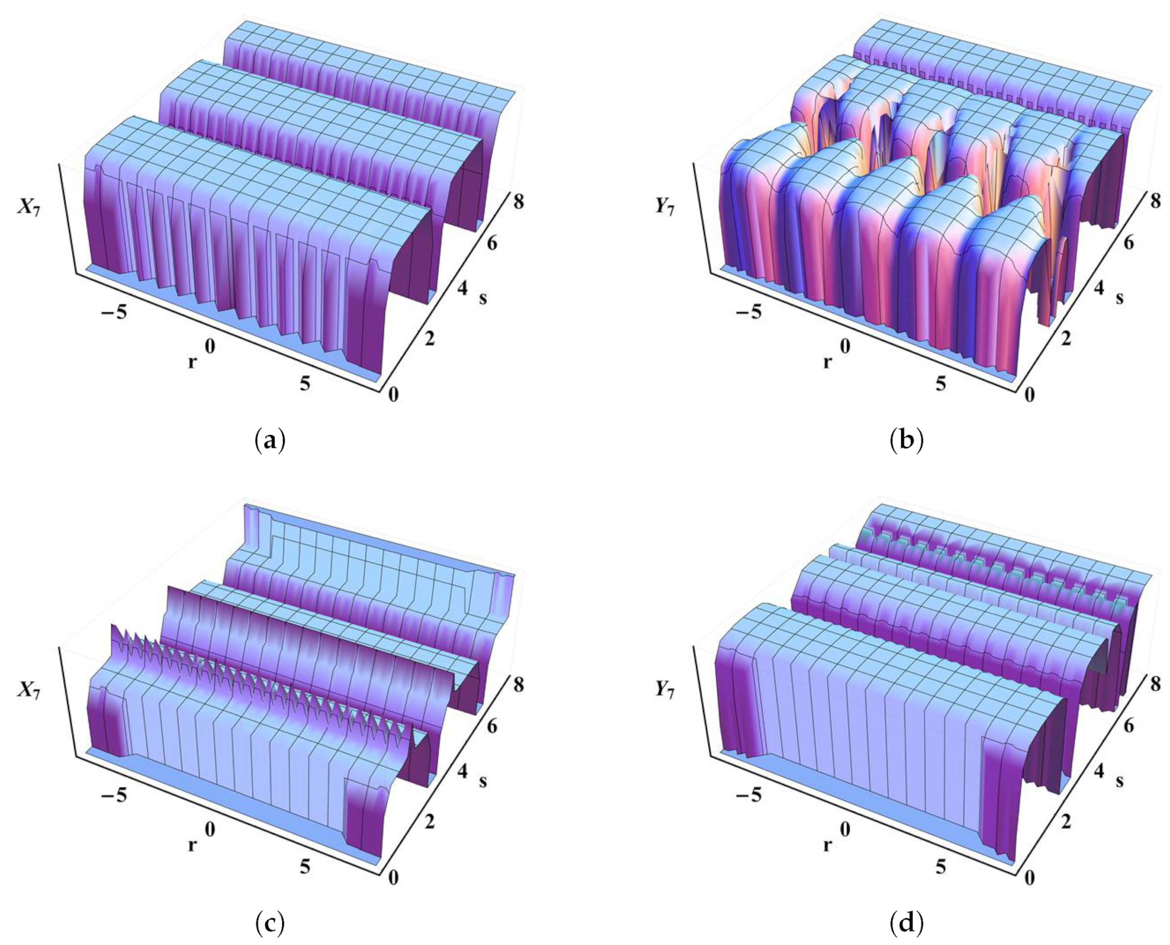
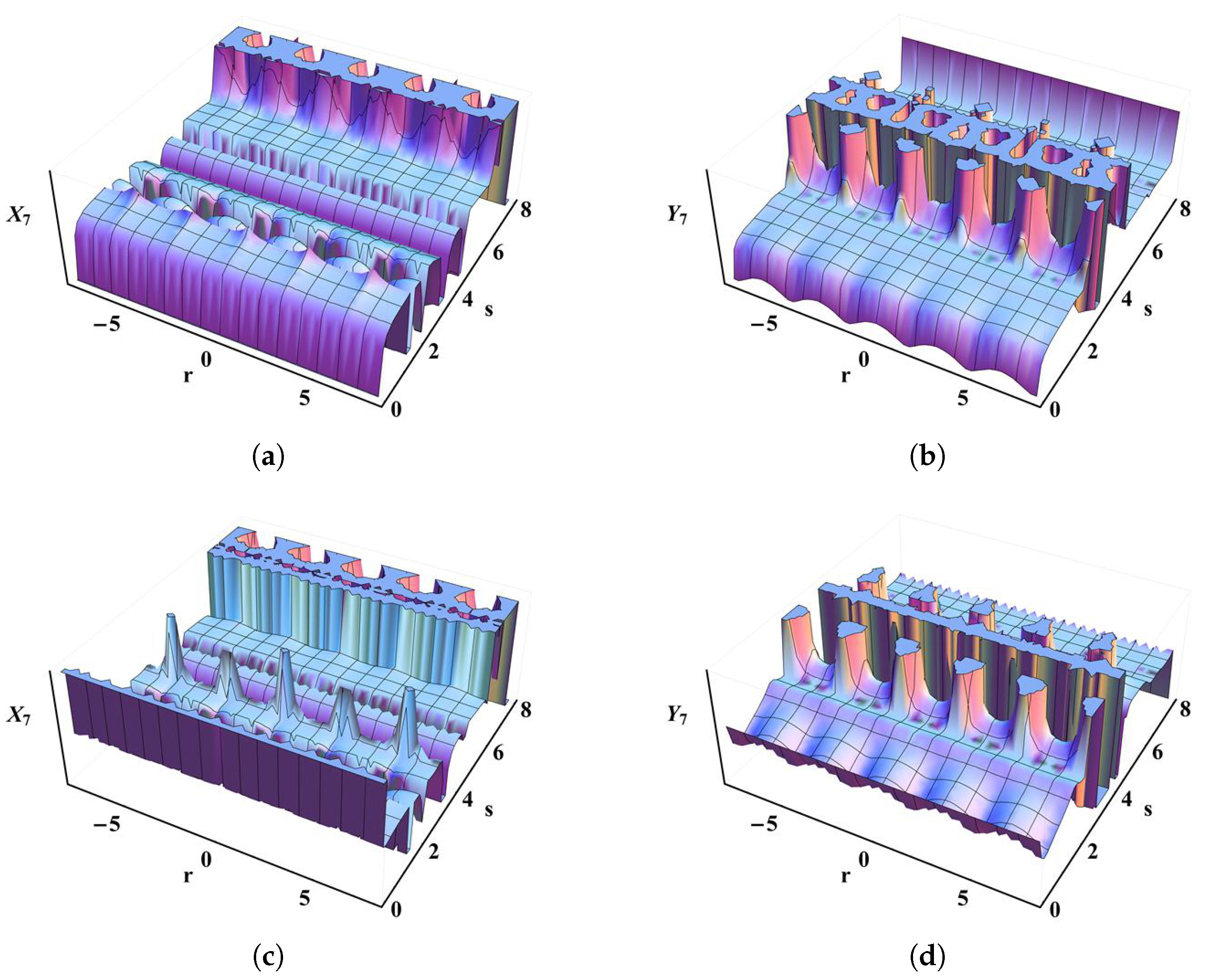
For $\pi =0.5$ and 1, the graphical interpretation of the solution (67)–(69) is presented in Figure 1 and Figure 2, when $R=S={\lambda }_1=2{\lambda }_2={\lambda }_3={\xi }_0={\xi }_1=4\alpha =1$, and $\delta \left(s\right)=r\left(s\right)={sin}^2\left(s\right)$. In the absence of the stochastic influence $\left(\mathbb{J}\right(s)=0)$, the evolutionary conduct of the solution (67)–(69) is shown in Figure 1. Figure 2 illustrates the stochastic evolutionary conduct of the solution (67)–(69) under the influence of the stochastic forces $\mathbb{J}\left(s\right)=tan\left(0.7s\right)\times \mathrm{Random}[0,1]$ and $\mathbb{I}\left(s\right)=0.7{sec}^2\left(0.7s\right)\times \mathrm{Random}[0,1]$. According to Figure 1 and Figure 2, one can conclude that the traveling wave amplitudes are unpredictable due to the stochastic driving components. Moreover, the aggregate impact of the generalized conformable derivatives may be depicted as a specific type of velocities whose directions are determined by the conformable parameter $\pi$.

Remark 1.

Many branches of nonlinear sciences rely heavily on wave solutions of nonlinear PDEs. The wave solutions of periodic and soliton kinds are the most often used wave solutions. In Equations (55)–(66), we have extracted new stochastic versions of periodic and soliton solutions for the stochastic CNKdV equations under recently generalized derivatives. The utility of periodic solutions appears in a variety of physical scopes, including collisionless plasmas, diffusion-advection systems impulsive systems, and more [41,42,43]. Moreover, the involvement of soliton solutions may also be seen in several physical areas, such as optical fibers, self-reinforcing systems, nuclear physics, controllability, and so on [44,45]. In actuality, the employed conformable derivatives lead to a particular rate of change relying on the conformable order π. So, depending on space, time, and the conformable order π, the acquired soliton and periodic solutions in (55)–(66) allow us to witness the slowdown or speedup in the monotonicity and symmetry of the researched stochastic nonlinear waves.

Remark 2.

It is clear that the extracted results are comprehensive and include many published results as special cases. For instances, if $\delta \left(s\right)=s$, the produced solutions (55)–(66) can be diminished to a new set of wave solutions for the stochastic CNKdV equations with the standard conformable derivatives of Khalil et al. [9]. Moreover, If $\pi =1$, the solutions (55)–(66) turn into a novel gathering of wave solutions for the stochastic CNKdV equations with traditional Newton’s derivatives [46].

6. Conclusions

In this article, we established deterministic and stochastic accurate solutions for the CNKdV equations with recently generalized conformable derivatives. New stochastic versions of periodic and soliton solutions for the these equations under conformable generalized derivatives were extracted. Some graphical interpretations and ultimate remarks were given to illustrate the stochastic evolutionary conduct of the solutions under the influence of the stochastic forces. It is notable that the presented solutions show the aggregate impact of the generalized conformable derivatives as specific type of velocities whose directions are determined by a conformable parameter. Moreover, we showed that the acceleration of the monotonicity and symmetry for the stochastic nonlinear wave solutions can be controlled via the conformable order $\pi$. Further, we gave a comparison between the wave solutions for the stochastic CNKdV equations under conformable generalized derivatives and the wave solutions constructed under the conformable derivatives of Khalil et al. [9] and Newton’s derivatives [46].

References

- Bhatti, M.M.; Marin, M.; Zeeshan, A.; Abdelsalam, S.I. Editorial: Recent Trends in Computational Fluid Dynamics. Front. Phys. 2020, 8, 593111. [Google Scholar] [CrossRef]
- Abdelrahman, M.A.E.; Sohaly, M.A.; Alharbi, A. The new exact solutions for the deterministic and stochastic(2+1)-dimensional equations in natural sciences. J. Taibah Univ. Sci. 2019, 13, 834–843. [Google Scholar] [CrossRef]
- Korpinar, Z.; Inc, M.; Bayram, M. Theory and application for the system of fractional Burger equations with Mittag leffler kernel. Appl. Math. Comp. 2020, 367, 124781. [Google Scholar] [CrossRef]
- Abouelregal, A.E.; Marin, M. The Size-Dependent Thermoelastic Vibrations of Nanobeams Subjected to Harmonic Excitation and Rectified Sine Wave Heating. Mathematics 2020, 8, 1128. [Google Scholar] [CrossRef]
- Podlubny, I. Fractional Differential Equation; Academic Press: San Diego, CA, USA, 1999. [Google Scholar]
- Uchaikin, V.V. Fractional Derivatives for Physicists and Engineers; Springer: Berlin/Heidelberg, Germany, 2013. [Google Scholar]
- Baleanu, D.; Diethelm, K.; Scalas, E.; Trujillo, J.J. Fractional Calculus: Models and Numerical Methods; World Scientific: Singapore, 2016. [Google Scholar]
- Anastassiou, G.A. Generalized Fractional Calculus: New Advancements and Applications; Springer: Cham, Swiztherland, 2021. [Google Scholar]
- Khalil, R.; Al Horani, M.; Yousef, A.; Sababheh, M. A new definition of fractional derivative. J. Comput. Appl. Math. 2014, 264, 65–70. [Google Scholar] [CrossRef]
- Zhao, D.; Luo, M. General conformable fractional derivative and its physical interpretation. Calcolo 2017, 54, 903–917. [Google Scholar] [CrossRef]
- Zhao, D.; Pan, X.; Luo, M. A new framework for multivariate general conformable fractional calculus and potential applications. Phys. A 2018, 510, 271–280. [Google Scholar] [CrossRef]
- Hyder, A.; Soliman, A.H. A new generalized θ-conformable calculus and its applications in mathematical physics. Phys. Scr. 2020, 96, 015208. [Google Scholar] [CrossRef]
- Hereman, W. Shallow Water Waves and Solitary Waves. In Mathematics of Complexity and Dynamical Systems; Meyers, R.G., Ed.; Springer: New York, NY, USA, 2012; pp. 1520–1532. [Google Scholar]
- Khismatullin, D.B.; Akhatov, I.S. Sound-ultrasound interaction in bubbly fluids: Theory and possible applications. Phys. Fluids 2001, 13, 3582–3598. [Google Scholar] [CrossRef]
- Crighton, D.G. Applications of KdV. In KdV ’95; Hazewinkel, M., Capel, H.W., de Jager, E.M., Eds.; Springer: Dordrecht, The Netherlands, 1995; pp. 39–67. [Google Scholar]
- Dodd, R.K.; Eilbeck, J.C.; Gibbon, J.D.; Morris, H.C. Solitons and Nonlinear Wave Equations; MR 696935; Academic Press, Inc. [Harcourt Brace Jovanovich, Publishers]: London, UK; New York, NY, USA, 1982. [Google Scholar]
- Drazin, P.G.; Johnson, R.S. Solitons: An introduction, Cambridge Texts in Applied Mathematics; MR 985322; Cambridge University Press: Cambridge, UK, 1989. [Google Scholar]
- Newell, A.C. Solitons in Mathematics and Physics; CBMS-NSF Regional Conference Series in Applied Mathematics, MR 847245; Society for Industrial and Applied Mathematics (SIAM): Philadelphia, PA, USA, 1985; Volume 48. [Google Scholar]
- Wazwaz, A. A two-mode modified KdV equation with multiple soliton solutions. Appl. Math. Lett. 2017, 70, 1–6. [Google Scholar] [CrossRef]
- Korsunsky, S.V. Soliton solutions for a second-order KdV equation. Phys. Lett. A 1994, 185, 174–176. [Google Scholar] [CrossRef]
- Hirota, R.; Satsuma, J. Soliton solutions of a coupled Korteweg-de Vries equation. Phys. Lett. A 1981, 85, 407–408. [Google Scholar] [CrossRef]
- Bouard, A.; Debussche, A. On the Stochastic Korteweg–de Vries Equation. J. Funct. Anal. 1998, 154, 215–251. [Google Scholar] [CrossRef]
- Hyder, A.; Barakat, M.A. General improved Kudryashov method for exact solutions of nonlinear evolution equations in mathematical physics. Phys. Scr. 2020, 95, 045212. [Google Scholar] [CrossRef]
- Hyder, A. White noise theory and general improved Kudryashov method for stochastic nonlinear evolution equations with conformable derivatives. Adv. Differ. Equ. 2020, 2020, 236. [Google Scholar] [CrossRef]
- Hyder, A.; Soliman, A.H. An extended Kudryashov technique for solving stochastic nonlinear models with generalized conformable derivatives. Commun. Nonlinear Sci. Numer. Simul. 2021, 97, 105730. [Google Scholar] [CrossRef]
- Kudryashov, N.A. One method for finding exact solutions of nonlinear differential equations. Commun. Nonlinear Sci. Numer. Simul. 2012, 17, 2248–2253. [Google Scholar] [CrossRef]
- Ren, Y.; Zhang, H. A generalized F-expansion method to find abundant families of Jacobi elliptic function solutions of the (2+1)-dimensional Nizhnik-Novikov-Veselov equation. Chaos Solitons Fract. 2006, 27, 959–979. [Google Scholar] [CrossRef]
- Dai, C.; Zhang, J. Jacobian elliptic function method for nonlinear differential difference equations. Chaos Solitons Fractals 2006, 27, 1042–1049. [Google Scholar] [CrossRef]
- Fan, E.; Zhang, J. Applications of the Jacobi elliptic function method to special-type nonlinear equations. Phys. Lett. A 2002, 305, 383–392. [Google Scholar] [CrossRef]
- Wang, M.; Zhang, J.; Li, X. The (G′/G)-expansion method and travelling wave solutions of nonlinear evolutions equations in mathematical physics. Phys. Lett. A 2008, 372, 417–423. [Google Scholar] [CrossRef]
- Özkan, E.M.; Özkan, A. On exact solutions of some important nonlinear conformable time-fractional differential equations. SeMA J. 2022, 1–16. [Google Scholar] [CrossRef]
- Behera, S.; Aljahdaly, N.H.; Virdi, J.P.S. On the modified (G′/G2)-expansion method for finding some analytical solutions of the traveling waves. J. Ocean Eng. Sci. 2022, 7, 313–320. [Google Scholar] [CrossRef]
- Ferdous, F.; Hafez, M.; Biswas, A.; Ekicid, M.; Zhoue, Q.; Alfirasf, M.; Moshokoac, S.P.; Belic, M. Oblique resonant optical solitons with Kerr and parabolic law nonlinearities and fractional temporal evolution by generalized exp(ϕ(ξ))-expansion. Optik 2019, 178, 439–448. [Google Scholar] [CrossRef]
- Ferdous, F.; Hafez, M. Nonlinear time fractional Kortewegde Vries equations for the interaction of wave phenomena in fluid-filled elastic tubes. Eur. Phys. J. Plus 2018, 133, 384. [Google Scholar] [CrossRef]
- Ferdous, F.; Hafez, M. Oblique closed form solutions of some important fractional evolution equations via the modified Kudryashov method arising in physical problems. J. Ocean Eng. Sci. 2018, 3, 244–252. [Google Scholar] [CrossRef]
- Akkurt, A.; Yildirim, M.E.; Yildirim, H. A new generalized fractional derivative and integral Konuralp. Konuralp J. Math. 2017, 5, 248–259. [Google Scholar]
- Aljahdaly, N.H. Some applications of the modified (G′/G2)-expansion method in mathematical physics. Results Phys. 2019, 13, 102272. [Google Scholar] [CrossRef]
- Das, P.K. New multi–hump exact solitons of a coupled Korteweg–de–Vries system with conformable derivative describing shallow water waves via RCAM. Phys. Scr. 2020, 95, 105212. [Google Scholar] [CrossRef]
- Grimshaw, R. Coupled Korteweg–de Vries equations. In Without Bounds: A Scientific Canvas of Nonlinearity and Complex Dynamics; Springer: Heidelberg, Germany, 2013; pp. 317–333. [Google Scholar]
- Holden, H.; sendal, B.; Ubøe, J.; Zhang, T. Stochastic Partial Differential Equations; Springer Science Media, LLC: New York, NY, USA, 2010. [Google Scholar]
- Allen, J.E.; Frantzeskakis, D.J.; Karachalios, N.I.; Kevrekidis, P.G.; Koukouloyannis, V. Solitary and periodic waves in collisionless plasmas: The Adlam-Allen model revisited. Phys. Rev. E 2020, 102, 013209. [Google Scholar] [CrossRef]
- Churilov, A.N. Orbital stability of periodic solutions of an impulsive system with a linear continuous-time part. AIMS Math. 2020, 5, 96–110. [Google Scholar] [CrossRef]
- Vidal-Henriquez, E.; Zykov, V.; Bodenschatz, E.; Gholami, A. Convective instability and boundary driven oscillations in a reaction-diffusion-advection model. Chaos Interdiscip. J. Nonlinear Sci. 2017, 27, 103110. [Google Scholar] [CrossRef] [PubMed]
- Melchert, O.; Demircan, A.; Yulin, A. Multi-frequency radiation of dissipative solitons in optical fiber cavities. Sci. Rep. 2020, 10, 8849. [Google Scholar] [CrossRef] [PubMed]
- Wang, G.; Yang, K.; Gu, H.; Guan, F.; Kara, A.H. A (2+1)-dimensional sine-Gordon and sinh-Gordon equations with symmetries and kink wave solutions. Nucl. Phys. B 2020, 953, 114956. [Google Scholar] [CrossRef]
- Xie, Y. Exact solutions for Wick-type stochastic coupled KdV equations. Phys. Lett. A 2004, 327, 174–179. [Google Scholar] [CrossRef]
Figure 1.
In the absence of the noise influence, (a,b) are 3D graphs for the solution (67)–(69) when , while, (c,d) are 3D graphs of the solution (67)–(69) when .
Publisher’s Note: MDPI stays neutral with regard to jurisdictional claims in published maps and institutional affiliations. |
© 2022 by the authors. Licensee MDPI, Basel, Switzerland. This article is an open access article distributed under the terms and conditions of the Creative Commons Attribution (CC BY) license (https://creativecommons.org/licenses/by/4.0/).
Share and Cite
MDPI and ACS Style
Hyder, A.-A.; Barakat, M.A.; Soliman, A.H.; Almoneef, A.A.; Cesarano, C. New Analytical Solutions for Coupled Stochastic Korteweg–de Vries Equations via Generalized Derivatives. Symmetry 2022, 14, 1770. https://doi.org/10.3390/sym14091770
AMA Style
Hyder A-A, Barakat MA, Soliman AH, Almoneef AA, Cesarano C. New Analytical Solutions for Coupled Stochastic Korteweg–de Vries Equations via Generalized Derivatives. Symmetry. 2022; 14(9):1770. https://doi.org/10.3390/sym14091770
Chicago/Turabian StyleHyder, Abd-Allah, Mohamed A. Barakat, Ahmed H. Soliman, Areej A. Almoneef, and Clemente Cesarano. 2022. "New Analytical Solutions for Coupled Stochastic Korteweg–de Vries Equations via Generalized Derivatives" Symmetry 14, no. 9: 1770. https://doi.org/10.3390/sym14091770
Note that from the first issue of 2016, this journal uses article numbers instead of page numbers. See further details here.