
Analytical Model of Heating an Isotropic Half-Space by a Moving Laser Source with a Gaussian Distribution


Moscow Aviation Institute, National Research University, 125993 Moscow, Russia
*
Author to whom correspondence should be addressed.
†
These authors contributed equally to this work.
Symmetry 2022, 14(4), 650; https://doi.org/10.3390/sym14040650
Submission received: 4 February 2022
/
Revised: 14 March 2022
/
Accepted: 19 March 2022
/
Published: 23 March 2022
(This article belongs to the Special Issue Foundations of Continuum Mechanics and Mathematical Physics)
Abstract
:This study presents the solution of the transient spatial problem of the impact of a moving source of heat flux induced by laser radiation on the surface of a half-space using the superposition principle and the method of transient functions. The solution is based on the Green’s function method, according to which the influence function of a surface-concentrated heat source is found at the first stage. The influence function has axial symmetry and the problem of finding the influence function is axisymmetric. To find the Green’s function, Laplace and Fourier integral transforms are used. The novelty of the obtained analytical solution is that the heat transfer at the free surface of the half-space is taken into account. The Green’s function that was obtained is used to construct an analytical solution to the moving heat-source problem in the integral form. The kernel of the advising integral operator is the constructed Green’s function. The Gaussian distribution is used to calculate integrals on spatial variables analytically. Gaussian law models the distribution of heat flux in the laser beam. As a result, the corresponding integrals on the spatial variables can be calculated analytically. A convenient formula that allows one to study the non-stationary temperature distribution when the heat source moves along arbitrary trajectories is obtained. A numerical, analytical algorithm has been developed and implemented that allows one to determine temperature distribution both on the surface and on the depth of a half-space. For verification purposes, the results were compared with the solution obtained using FEM.
1. Introduction
Additive manufacturing is an alternative way of producing finished products of different geometries and purposes. In contrast to traditional methods of producing, the process of creating geometry by 3D printing methods with metal–powder compositions is accompanied by high-intensity heating of the synthesized material. Emerging temperature fields can have a significant impact on the microstructure and properties of the material, as well as on the magnitude and nature of the residual stresses and strains [1,2,3]. The use of analytical methods for solving temperature problems has a significant advantage over numerical methods. The analytical solution provides significantly faster and more accurate results. In addition, it simplifies the investigation into the influence of various problem parameters on the thermal heating process. This makes it possible to predict and identify areas of high temperature at the design stage [4,5]. During the three-dimensional printing process, the material experiences significant temperature fluctuations which result in undesirable thermal stresses and residual stresses [6].
It is possible to use hyperbolic-type equations to solve this problem. Various aspects of research into solutions of such equations are presented in papers [7,8,9,10]. However, constructing a solution to the parabolic heat-conduction equation is significantly simpler. In addition, the results obtained were compared with the solution of the test problem using the finite element method. A good coincidence of the obtained results was revealed. Therefore, the parabolic-type heat-conduction equation was used in the work.
In this paper, we have developed an analytical method for determining the thermal field created in a semi-infinite body by a moving heat source distributed over the heating spot by a symmetric Gaussian distribution function. The solution is based on the Green’s function method, according to which the influence function of a surface-concentrated heat source (Green’s function) is found first. In [7,8,9], the influence function method has been used to solve non-stationary contact problems for shells and solid bodies. In [10], the authors used Green’s functions in the contact problem for a spherical shell and an absolutely solid surface. The shell was created using additive technologies. Comparison with experimental results has been carried out, and a good coincidence of the obtained results has been shown. In [11,12], Green’s functions have been used to solve problems of moving surface loading on an elastic half-space and also in analytical studies of peculiarities of solutions of non-stationary contact problems [13,14,15,16].
In this paper, the problem of constructing the influence function of a surface heat source is solved using integral Fourier and Laplace transforms. In this case, the obtained solution allows us to take into account the heat transfer at the surface, which is a new result. Then, using the superposition principle, the solution of the original problem is determined.
By now, there is a fairly large number of publications on the study of the temperature field induced by a moving heat source. Works such as [17,18] solve stationary problems about a moving heat source. The Green’s function for a volumetric heat source was used. Similar problems, but in a non-stationary formulation, are considered in [19,20,21,22,23]. In these works, the solution is constructed using analytical methods. However, a significant drawback is the use of Green’s function for unbounded space in the solution. Thus, these works automatically exclude the influence of the presence of a boundary surface, since initially, when building the Green’s function, the problem is solved without boundary conditions on the free surface of a half-space. Thus, for example, the influence of heat exchange with the environment on the boundary surface is not taken into account.
The volumetric influence function is also used to describe the material welding process [23,24,25]. Although the welding process is different from the 3D printing process, the physical processes are very similar.
In work [24], the one-dimensional problem of the motion of a heat source is solved. The author investigates the temperature distribution in the vicinity of a rectangular-shaped source moving with constant velocity along the rod axis. The unsteady temperature field from the moving heat source was constructed using a Fourier series. Approaches to solving two- and three-dimensional problems using the apparatus of Fourier series and finite integral transformations have been developed in [25,26]. Though the mathematical apparatus used is rigorous, there remain questions concerning the control of the convergence of the constructed decompositions. In addition, these works introduce some simplifying provisions concerning the consideration of the influence of heat exchange on the surface. In addition, the simplest variant of the heat-source motion, a uniform rectilinear motion, is also considered.
In contrast to these works, this publication finds and uses a new function of the influence of the surface heat source, taking into account the process of heat exchange with the environment through the boundary surface. Previously, this function has not been used in solving problems of this type. In addition, in all known works, as a rule, only one simplest case of motion of a heat source —uniform rectilinear motion with a given velocity along one of the axes of the coordinate system–is considered. In this paper, a convenient formula has been obtained that allows for calculating the three-dimensional unsteady temperature field induced by a moving source moving along any trajectory arbitrarily dependent on time. It is an exact analytical solution without the use of any simplifying assumptions.
Thus, the method proposed in this work allows us to obtain the most accurate three-dimensional temperature distribution when exposed to a laser emitter moving along complex curves with varying speed, as happens in three-dimensional printing processes by selective laser melting technology. Calculation examples are given. The obtained results are compared with the results of numerical solutions by means of the finite element method. It is shown that the analytical solution agrees well with the numerical one.
2. Problem Statement
Assume that at the initial time moment at the origin of the rectangular Cartesian coordinate system related to the surface of the half-space heat source q begins to act and moves across the surface of the half-space according to an arbitrary law in time (Figure 1). The flux density q is distributed over the heating spot of radius R; in general, it can depend both on the radius and time:
where is the Heaviside distribution.
The coordinates of the heating spot center at the moments of time are determined by the parametric dependences:
The medium filling the half-space is characterized by specific heat capacity c, mass density , and thermal conductivity coefficient . Consider that the medium is homogeneous and isotropic, and that the density and thermophysical constants are constants. Assume also the absence of volumetric heat sources in the half-space. In this case, the temperature distribution in the medium follows the thermal conductivity equation [27,28]:
where denotes the diffusivity.
At the initial time moment (), the temperature at all points of the half-space vanishes:
The boundary conditions of the third kind are formulated on the surface of the half-space [5,28]. Taking into account (1) and (2), one could formulate them as follows:
The temperature is considered to be bounded at infinity:
3. Solution Method
The problem of a concentrated heat source applied to the surface of a half-space can be represented in the following form:
where is the Dirac delta distribution.
The solution of problem (7) can be called the surface heat-source transient function. Hereinafter, we refer to it simply as the surface transient function.
Based on the superposition principle [11,12,13,14,15,16], the solution of the initial problem (3)–(6) can be considered as a convolution of the transient function with the right-hand side of the boundary condition (5) for the variables x, y and for time:
Thus, the key point is to build the transient function of the surface source. To solve this problem, let us apply to (7) the Laplace integral transform in time with a parameter s and the Fourier integral transforms in spatial variables x and y with the corresponding parameters and :
A bounded solution at of Equation (9) is:
The constant A is found from the first boundary condition (10):
The result is:
To find the original, first inverse the Laplace transform:
and then successively Fourier transforms.
Thus, we obtain the original surface transient function in the form:
The solution of the moving heat-source problem is expressed by the triple integral (8) and presents certain difficulties associated with calculating the double integral on spatial variables, therefore we propose the following solution approach.
Let us move to a moving coordinate system connected with the center of the heating spot in Formula (8). Thus, we have:
Consider that the distribution of the heat flux q over the surface of the half-space is independent of time and obeys the Gaussian distribution law:
where Q—laser source power, —standard deviation.
Based on the property of the Gaussian function .
By choosing one or another value of the standard deviation , one can adjust the radius of the heating spot carrier.
Figure 2 shows the graphs of the function , at different values of . The solid curve corresponds to , hatch–, dashed–.
The figure shows that the value of should be taken as equal to . This agrees with the well-known rule of three sigma, according to which almost all values of a quantity with probability 0.9973 lie no further than three sigmas to either side of the mathematical expectation in a normal distribution, which in this case is equal to zero.
Figure 3 shows the three-dimensional distribution when .
Note that the impact function is the product of two factors, the first of which depends only on z and t, and the second depends on x, y and t:
Taking into account (18), let us represent Formula (16) in the form:
Consider the integral :
After some transformations:
Given the equality of we obtain:
Taking into account the heat transfer on the surface, the formula for the temperature field induced by a moving laser source takes the form of a one-dimensional integral over time:
4. Results
Examine the case where the spot of the laser source of radius microns and power Q = 300 W moves along the surface of the half-space along a rectilinear segment of length L along the axis X with a constant velocity v = 1600 mm/s. For this case, the surface plot of the temperature distribution at the last moment of time is shown in Figure 4. Temperature distribution over the surface along the trajectory of the spot on the surface for the last moment of time is shown in Figure 5. It can be seen that the maximum temperature corresponds to the exposure spot of the heating source. The maximum temperature is reached at the centre of the heating spot, as the temperature decreases quite sharply away from the centre. Figure 5 shows the surface temperature distribution along the path of the surface heat source.
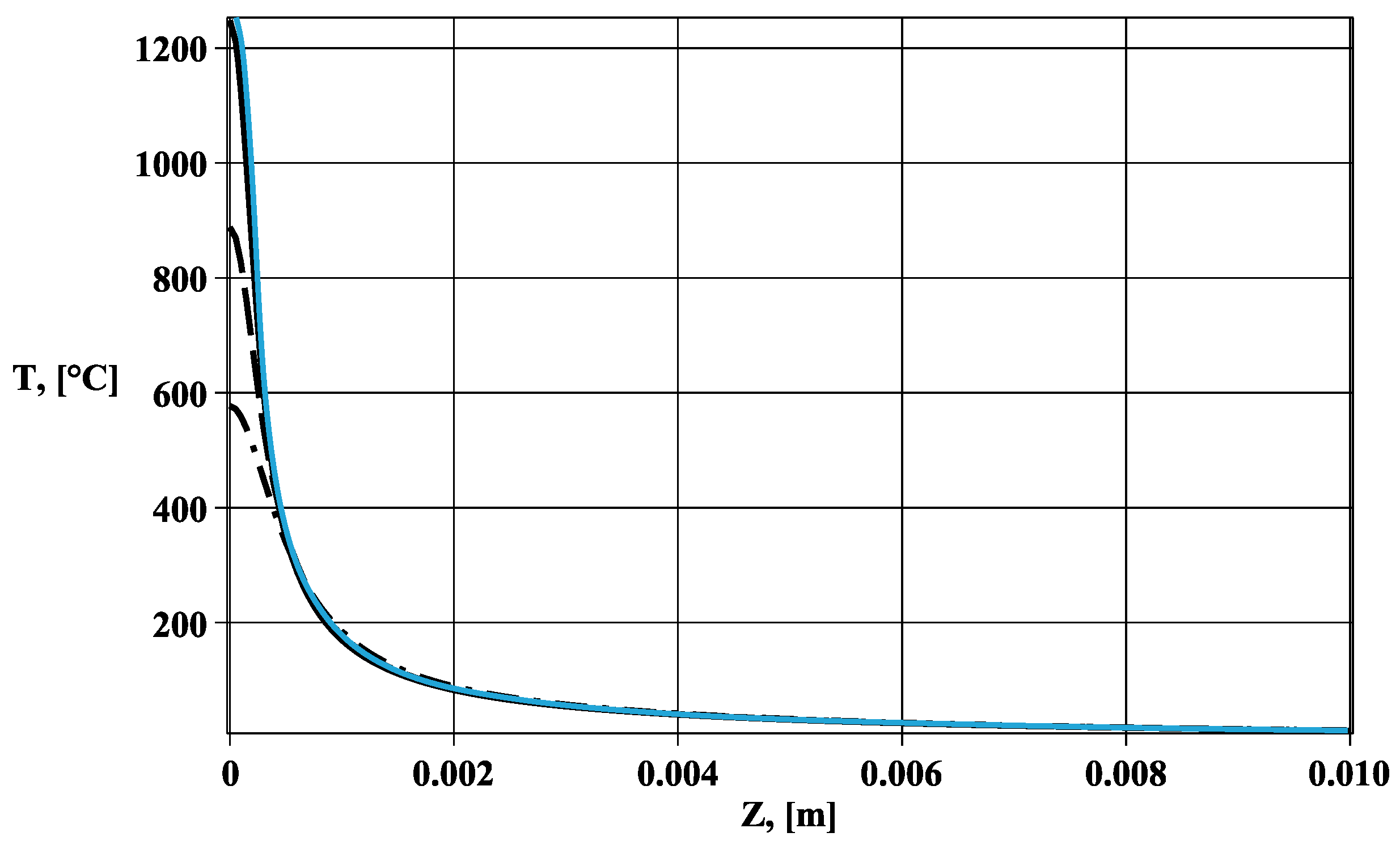
The graph of temperature distribution along the depth at the point of laser exposure at the last moment of time is shown in Figure 6.
The graph in Figure 6 shows that the maximum temperature is noticeably lower at a distance from the heat flux, but that there is no complete cooling.
Now, assume that the spot from the laser light source moves along a given complex trajectory shown in Figure 7.
Figure 8 and Figure 9 show the results of calculations of the temperature distribution along the trajectory of the spot on the surface at the last moment and in depth at various points at the last moment of time.
The graph in Figure 8 shows that there are sharp temperature increases. This is due to the fact that the laser source during the trajectory can cross or be in the vicinity of points that have already been exposed to it.
5. Conclusions
An analytical model for determining the temperature field arising in the process of selective laser melting has been developed. The spatial transient problem of the impact of a moving source of heat flux on the surface of a half-space is solved using the superposition principle and the method of transient functions. The solution is constructed as a quadrature. The kernel of the corresponding integral operator is the surface heat-source transient function constructed using the Fourier and Laplace integral transforms. This mathematical model makes it possible to determine the temperature distribution not only in the vicinity of the heating spot on the surface of the half-space, but also along the depth, which is important when modeling three-dimensional printing processes.
The developed solution method can be applied to solving problems of uncoupled thermoelasticity to determine the residual temperature stresses under the influence of mobile surface heat sources.
Calculation results are obtained for rectilinear and complex trajectory cases. The results are shown in graphs.
Author Contributions
Conceptualization, A.O., L.R. and G.F.; methodology, A.O., L.R. and G.F.; software, A.O., L.R. and G.F.; validation, A.O., L.R. and G.F.; formal analysis, A.O., L.R. and G.F.; investigation, A.O., L.R. and G.F.; resources, A.O., L.R. and G.F.; data curation, A.O., L.R. and G.F.; writing—original draft preparation, A.O., L.R. and G.F.; writing—review and editing, A.O., L.R. and G.F.; visualization, A.O., L.R. and G.F.; supervision, A.O., L.R. and G.F.; project administration, A.O., L.R. and G.F.; funding acquisition, A.O., L.R. and G.F. All authors have read and agreed to the published version of the manuscript.
Funding
The work was financially supported by the Ministry of Science and Higher Education of the Russian Federation (project code FSFF-2020-0017).
Institutional Review Board Statement
Not applicable.
Informed Consent Statement
Not applicable.
Data Availability Statement
Not applicable.
Conflicts of Interest
The authors declare no conflict of interest.
References
- Mirkoohi, E.; Dobbs, J.R.; Liang, S.Y. Analytical mechanics modeling of in-process thermal stress distribution in metal additive manufacturing. J. Manuf. Process. 2020, 58, 41–45. [Google Scholar] [CrossRef]
- Babaytsev, A.; Dobryanskiy, V.; Solyaev, Y. Optimization of Thermal Protection Panels Subjected to Intense Heating and Mechanical Loading. Lobachevskii J. Math. 2019, 40, 887–895. [Google Scholar] [CrossRef]
- Fergani, O.; Berto, F.; Welo, T.; Liang, S.Y. Analytical modelling of residual stress in additive manufacturing. Fatigue Fract. Eng. Mater. Struct. 2017, 40, 971–978. [Google Scholar] [CrossRef]
- Tushavina, O.V. Coupled heat transfer between a viscous shock gasdynamic layer and a transversely streamlined anisotropic half-space. INCAS Bull. 2020, 12, 211–220. [Google Scholar] [CrossRef]
- Pronina, P.F.; Sun, Y.; Tushavina, O.V. Mathematical modelling of high-intensity heat flux on the elements of heat-shielding composite materials of a spacecraft. J. Appl. Eng. Sci. 2020, 18, 693–698. [Google Scholar] [CrossRef]
- Kruth, J.; Deckers, J.; Yasa, E.; Wauthlé, R. Assessing and comparing influencing factors of residual stresses in selective laser melting using a novel analysis method. Proc. Inst. Mech. Eng. Part B J. Eng. Manuf. 2012, 226, 980–991. [Google Scholar] [CrossRef]
- Matevossian, H.; Nordo, G.; Vestyak, A. Behavior of Solutions of the Cauchy Problem and the Mixed Initial Boundary Value Problem for an Inhomogeneous Hyperbolic Equation with Periodic Coefficients. In Developments and Novel Approaches in Nonlinear Solid Body Mechanics, Chapter 4, Advanced Structured Materials; Springer: Cham, Switzerland, 2020; Volume 130, pp. 29–35. [Google Scholar]
- Matevossian, H.; Vestyak, A.; Peshcherikova, O. On the behavior of solutions of the initial boundary value problems for the hyperbolic equation with periodic coefficients. Math. Notes 2018, 104, 762–766. [Google Scholar] [CrossRef]
- Vestyak, A.; Matevossian, H. On the behavior of the solution of the Cauchy problem for an inhomogeneous hyperbolic equation with periodic coefficients. Math. Notes 2017, 102, 424–428. [Google Scholar] [CrossRef]
- Vestyak, A.; Matevossian, H. On the behavior of the solution of the Cauchy problem for a hyperbolic equation with periodic coefficients. Math. Notes 2016, 100, 751–754. [Google Scholar] [CrossRef]
- Mikhailova, E.; Fedotenkov, G.; Tarlakovskii, D. Impact of Transient Pressure on a Half-Space with Membrane Type Coating. Struct. Integr. 2020, 16, 312–315. [Google Scholar]
- Fedotenkov, G.; Tarlakovskii, D. Non-stationary Contact Problems for Thin Shells and Solids. Struct. Integr. 2020, 16, 287–292. [Google Scholar]
- Okonechnikov, A.; Fedotenkov, G.; Tarlakovskii, D. Spatial non-stationary contact problem for a cylindrical shell and absolutely rigid body. Mech. Solids 2020, 55, 366–376. [Google Scholar] [CrossRef]
- Fedotenkov, G.V.; Mikhailova, E.Y.; Kuznetsova, E.L.; Rabinskiy, L.N. Modeling the unsteady contact of spherical shell made with applying the additive technologies with the perfectly rigid stamp. Int. J. Pure Appl. Math. 2016, 111, 331–342. [Google Scholar] [CrossRef] [Green Version]
- Igumnov, L.A.; Okonechnikov, A.S.; Tarlakovskii, D.V.; Fedotenkov, G.V. Plane Nonstationary Problem of Motion of the Surface Load Over an Elastic Half Space. J. Math. Sci. 2014, 203, 193–201. [Google Scholar] [CrossRef]
- Tarlakovskiy, D.V.; Fedotenkov, G.V. Analytic investigation of features of stresses in plane nonstationary contact problems with moving boundaries. J. Math. Sci. 2009, 162, 246–253. [Google Scholar] [CrossRef]
- Hou, Z.B.; Komanduri, R. General solutions for stationary/moving plane heat source problems in manufacturing and tribology. Int. J. Heat Mass Transf. 2020, 43, 1679–1698. [Google Scholar] [CrossRef]
- Ramos-Grez, J.A.; Sen, M. Analytical, quasi-stationary wilson-rosenthal solution for moving heat sources. Int. J. Therm. Sci. 2019, 140, 455–465. [Google Scholar] [CrossRef]
- Ghosh, A.; Chattopadhyay, H. Mathematical modeling of moving heat source shape for submerged arc welding process. Int. J. Adv. Manuf. Technol. 2013, 69, 2691–2701. [Google Scholar] [CrossRef]
- Parkitny, R.; Winczek, J. Analytical solution of temporary temperature field in half-infinite body caused by moving tilted volumetric heat source. Int. J. Heat Mass Transf. 2013, 60, 469–479. [Google Scholar] [CrossRef]
- Komanduri, R.; Hou, Z.B. Thermal analysis of the arc welding process: Part I. general solutions. Metall. Mater. Trans. B Process. Metall. Mater. Process. Sci. 2000, 31, 1353–1370. [Google Scholar] [CrossRef]
- Komanduri, R.; Hou, Z.B. Thermal analysis of the arc welding process: Part II. effect of variation of thermophysical properties with temperature. Metall. Mater. Trans. B Process. Metall. Mater. Process. Sci. 2001, 32, 483–499. [Google Scholar] [CrossRef]
- Nguyen, N.T.; Ohta, A.; Matsuoka, K.; Suzuki, N.; Maeda, Y. Analytical solutions for transient temperature of semi-infinite body subjected to 3-D moving heat sources. Weld. J. (Miami Fla) 1999, 78, 265–274. [Google Scholar]
- Kim, C.K. An analytical solution to heat conduction with a moving heat source. J. Mech. Sci. Technol. 2011, 25, 895–899. [Google Scholar] [CrossRef]
- Salimi, S.; Bahemmat, P.; Haghpanahi, M. An analytical solution to the thermal problems with varying boundary conditions around a moving source. Appl. Math. Model. 2016, 40, 6690–6707. [Google Scholar] [CrossRef]
- Araya, G.; Gutierrez, G. Analytical solution for a transient, three-dimensional temperature distribution due to a moving laser beam. Int. J. Heat Mass Transf. 2006, 49, 4124–4131. [Google Scholar] [CrossRef]
- Carslaw, H.; Jaeger, J. Conduction of Heat in Solids, 2nd ed.; Clarendon Press: Oxford, UK, 1959. [Google Scholar]
- Lykov, A. Teoriya Teploprovodnosti; Vysshaya Shkola: Moscow, Russia, 1967. [Google Scholar]
Figure 1.
Heating of a half-space by a moving heat source.

Figure 2.
Heat flux distributions at different values .
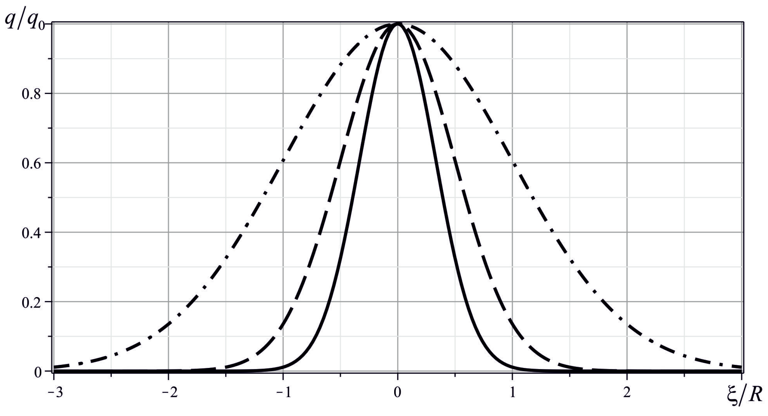
Figure 3.
Spatial distribution of laser radiation flux at .

Figure 4.
Temperature distribution over the surface at the last moment of time.
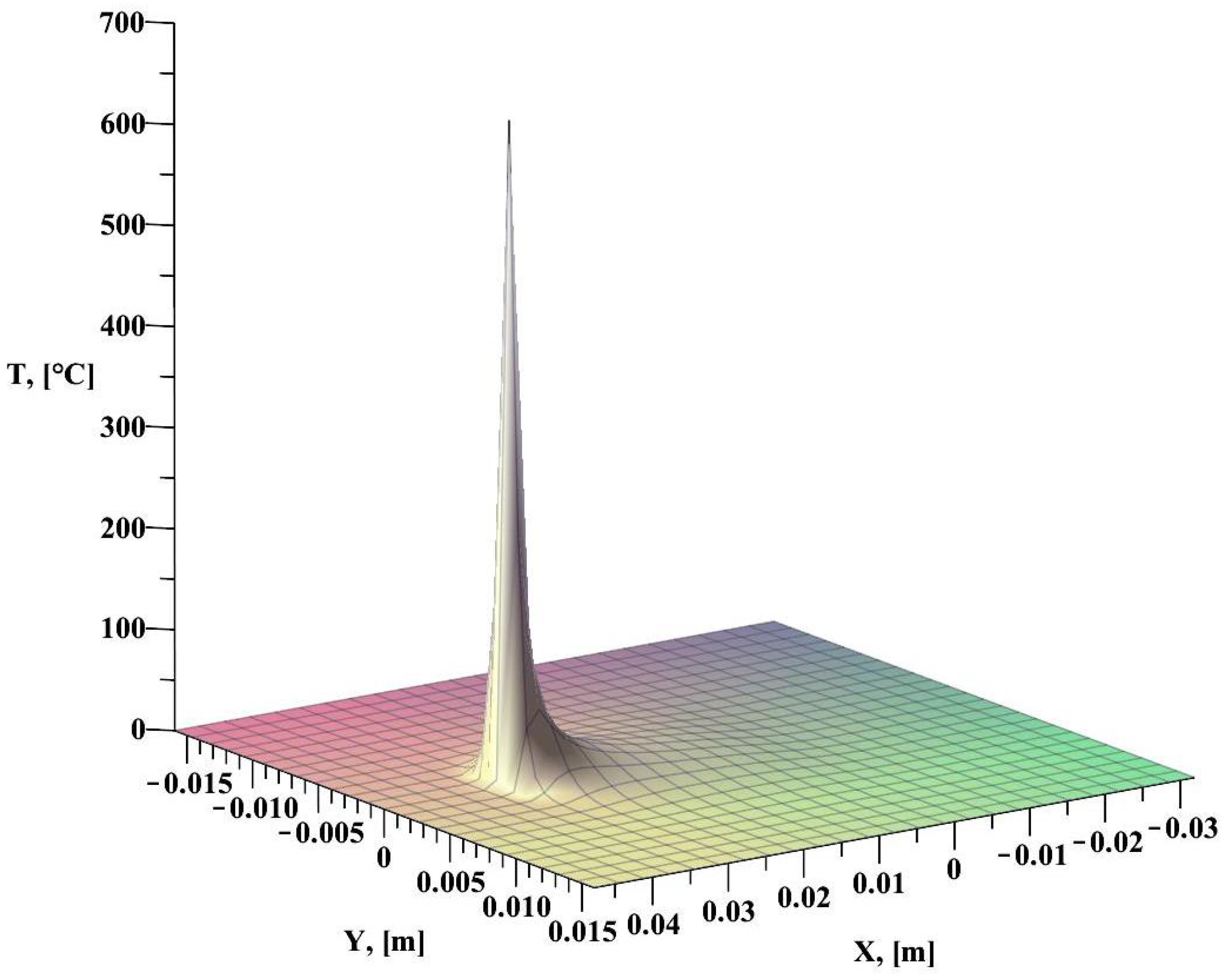
Figure 5.
Temperature distribution over the surface along the trajectory of the spot on the surface at the last moment of time.
Figure 5.
Temperature distribution over the surface along the trajectory of the spot on the surface at the last moment of time.

Figure 6.
Temperature distribution along the depth at the last moment of time. The solid line corresponds to x = L; the hatched line to x = 0.99 L; the dashed line to x = 0.77 L, where L is the length of the trajectory. Blue line corresponds to numerical simulation.
Figure 6.
Temperature distribution along the depth at the last moment of time. The solid line corresponds to x = L; the hatched line to x = 0.99 L; the dashed line to x = 0.77 L, where L is the length of the trajectory. Blue line corresponds to numerical simulation.
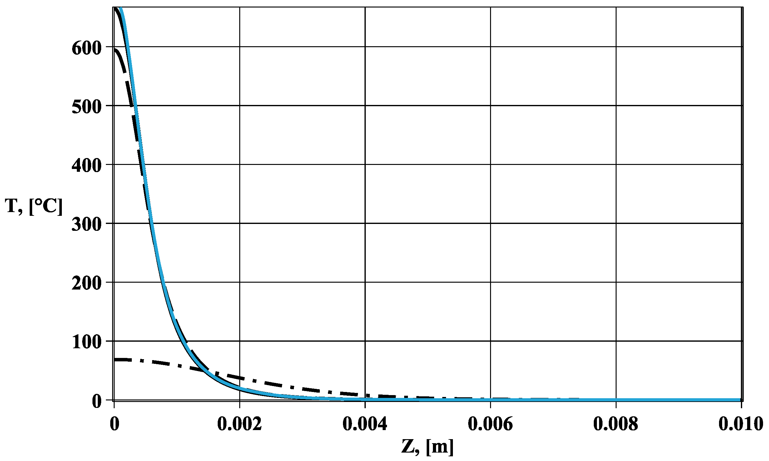
Figure 7.
Trajectory of the spot on the surface.

Figure 8.
Temperature distribution along the trajectory of the spot on the surface at the last moment of time.
Figure 8.
Temperature distribution along the trajectory of the spot on the surface at the last moment of time.
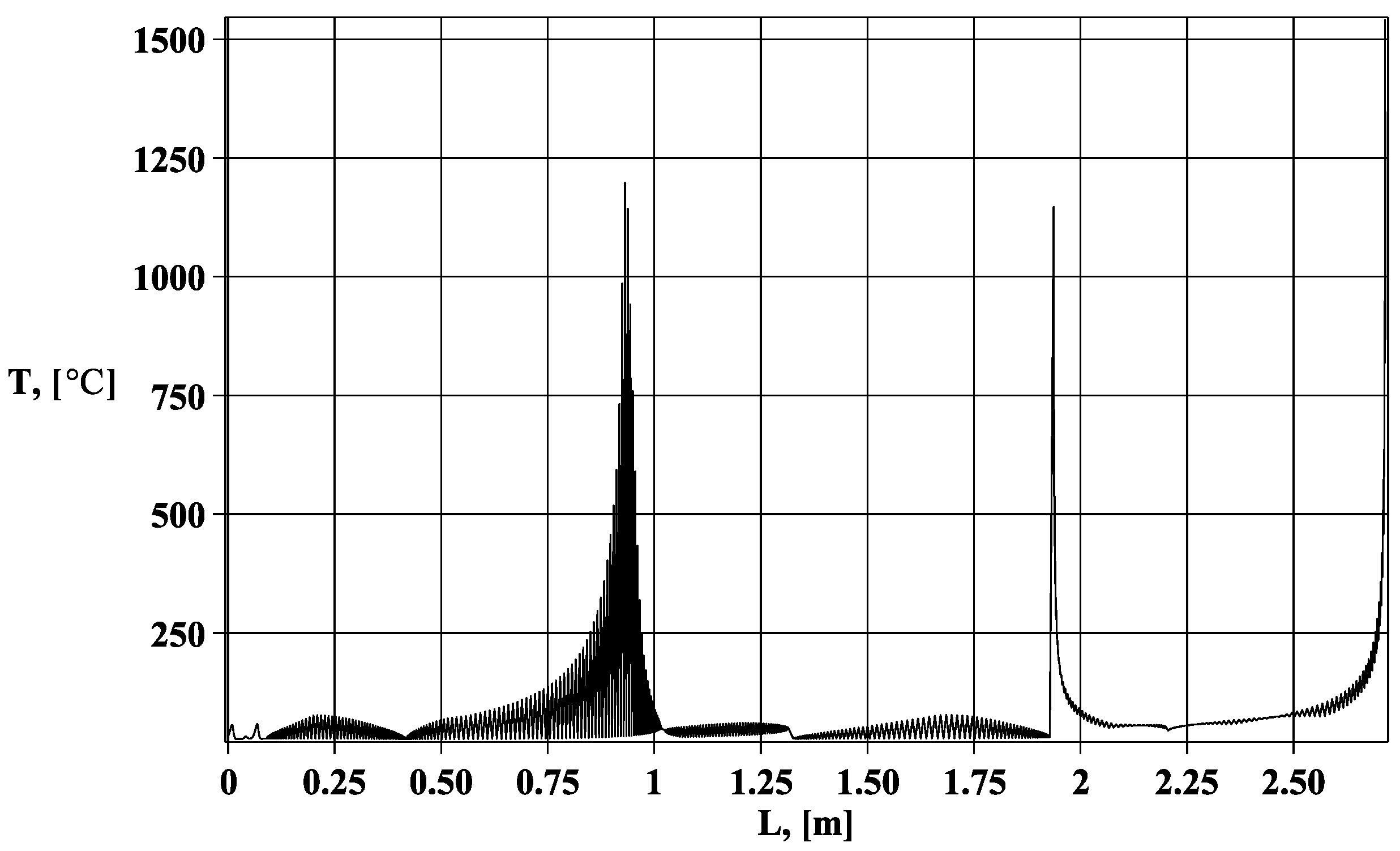
Figure 9.
Temperature distribution along the depth at the last moment of time. The solid line corresponds to L; the hatched line to 0.99 L; the dashed line to 0.77 L. Blue line corresponds to numerical simulation.
Figure 9.
Temperature distribution along the depth at the last moment of time. The solid line corresponds to L; the hatched line to 0.99 L; the dashed line to 0.77 L. Blue line corresponds to numerical simulation.
Publisher’s Note: MDPI stays neutral with regard to jurisdictional claims in published maps and institutional affiliations. |
© 2022 by the authors. Licensee MDPI, Basel, Switzerland. This article is an open access article distributed under the terms and conditions of the Creative Commons Attribution (CC BY) license (https://creativecommons.org/licenses/by/4.0/).
Share and Cite
MDPI and ACS Style
Orekhov, A.; Rabinskiy, L.; Fedotenkov, G. Analytical Model of Heating an Isotropic Half-Space by a Moving Laser Source with a Gaussian Distribution. Symmetry 2022, 14, 650. https://doi.org/10.3390/sym14040650
AMA Style
Orekhov A, Rabinskiy L, Fedotenkov G. Analytical Model of Heating an Isotropic Half-Space by a Moving Laser Source with a Gaussian Distribution. Symmetry. 2022; 14(4):650. https://doi.org/10.3390/sym14040650
Chicago/Turabian StyleOrekhov, Alexander, Lev Rabinskiy, and Gregory Fedotenkov. 2022. "Analytical Model of Heating an Isotropic Half-Space by a Moving Laser Source with a Gaussian Distribution" Symmetry 14, no. 4: 650. https://doi.org/10.3390/sym14040650
Note that from the first issue of 2016, this journal uses article numbers instead of page numbers. See further details here.