Multiplicative Brownian Motion Stabilizes the Exact Stochastic Solutions of the Davey–Stewartson Equations

Abstract

In this article, the stochastic Davey–Stewartson equations (SDSEs) forced by multiplicative noise are addressed. We use the mapping method to find new rational, elliptic, hyperbolic and trigonometric functions. In addition, we generalize some previously obtained results. Due to the significance of the Davey–Stewartson equations in plasma physics, nonlinear optics, hydrodynamics and other fields, the discovered solutions are useful in explaining a number of intriguing physical phenomena. By using MATLAB tools to simulate our results and display some of 3D graphs, we show how the multiplicative Brownian motion impacts the analytical solutions of the SDSEs. Finally, we demonstrate the effect of multiplicative Brownian motion on the stability and the symmetry of the achieved solutions of the SDSEs.

1. Introduction

The majority of nonlinear physical phenomena that occur in a variety of scientific areas, including chemical kinetics, optical fibers, fluid dynamics, solid-state physics and mathematical biology, may be modeled via nonlinear partial differential equations (PDEs). The investigate of the analytical solutions of these PDEs is critical for comprehension most nonlinear physical phenomena and their applications. Various approaches for discovering the analytical solutions of PDEs have been presented to overcome this issue. Some examples of the most significant methods are tanh-sech [1,2,3], extended tanh-function [4], the Sine-Gordon expansion [5], the trial function [6], the Darboux transformation [7], the Jacobi elliptic function [8,9], the sine-cosine [10,11], $(G^{\prime }/G)$-expansion [12,13], Hirota’s function [14], $exp(-\varphi (\varsigma \left)\right)$-expansion [15], perturbation [16,17], the qualitative theory of dynamical systems [18,19,20,21], the direct method [22], the Riccati–Bernoulli sub-ODE [23], and the F-expansion method [24].

On the other side, the advantages of taking random influences into account in the analysis, simulation, prediction and modeling of complex processes have been highlighted in several fields including chemistry, geophysics, fluid mechanics, biology, atmosphere, physics, climate dynamics, engineering and other fields [25,26,27,28]. Since noise may produce statistical features and significant phenomena, it cannot be ignored. In general, it is more difficult to obtain exact solutions to PDEs forced by stochastic terms than to obtain those to classical ones.

The Davey–Stewartson equations affected by multiplicative noise in the Stratonovich sense are taken into consideration as follows:

$$\begin{array}{ccc}\hfill i{u}_t+\frac{1}{2}{\delta }^2(u_{xx}+{\delta }^2{u}_{yy})+\kappa {\left|u\right|}^{2}u-uv+i\sigma u\circ B_t& =& 0,\hfill \end{array}$$

(1)

$$\begin{array}{ccc} \hfill v_{xx}-{\delta }^2{v}_{yy}-2\kappa {({\left|u\right|}^2)}_{xx}& =& 0,\hfill \end{array}$$

(2)

where $u(x,y,t)\in \mathbb{C}$, $v(x,y,t)\in \mathbb{R}$, $\kappa =\pm 1$ and ${\delta }^2=\pm 1.$ The constant $\kappa$ measures the cubic nonlinearity. The case $\delta =1$ is known as the DS-I equation, while $\delta =i$ is known as the DS-II equation. They occur in a variety of applications, including the description of gravity–capillary surface wave packets in shallow water. $B\left(t\right)$ is Brownian motion, and $\sigma$ is the strength of the noise.

We notice that there are various ways such as the Itô and Stratonovich calculus to interpret the stochastic integral ${\int }_0^{t}YdB$. The stochastic integral is Itô (indicated by ${\int }_0^{t}YdB$) when it is assessed at the left-end as opposed to a Stratonovich stochastic integral (indicated by ${\int }_0^{t}Y\circ dB$), which is computed in the center [29]. The following equation is how the Itô integral and Stratonovich integral are related:

$${\int }_0^{t}Y\left(Z_{\tau }\right)dB\left(\tau \right)={\int }_0^{t}Y\left(Z_{\tau }\right)\circ dB\left(\tau \right)-\frac{1}{2}{\int }_0^{t}Y\left(Z_{\tau }\right)\frac{\partial Y\left(Z_{\tau }\right)}{\partial z}d\tau ,$$

(3)

where Y is supposed to be sufficiently regular and $\{Z_t,$$t\ge 0\}$ is a stochastic process.

The Davey–Stewartson equation was created in 1974 by Davey and Stewartson [30]. This equation is employed to demonstrate how a three-dimensional wave packet evolves over time in a restricted depth of water. The solutions of the deterministic Davey–Stewartson equations (DDSEs) (1) and (2), i.e., $\sigma =0$, have been used in hydrodynamics, nonlinear optics, plasma physics and other fields. For example, the solutions of the DDSEs might explain the interaction of a properly matched spatiotemporal optical pattern and microwaves. As a result, many authors have investigated the analytical solutions for this equation by using different methods such as the extended Jacobi’s elliptic function [31], the first integral method [32], the trial equation method [33], the uniform algebraic method [34], the double exp-function [35], generalized $(G^{\prime }/G)$-expansion [36], $(G^{\prime }/G)$-expansion [37] and sine–cosine [38].

Our motivation in this paper is to attain the analytical solutions of the stochastic Davey–Stewartson equations (SDSEs). This work is the first to obtain the analytical solutions of SDSEs (1) and (2). We employ the mapping method to obtain a wide range of stochastic solutions, such as rational, elliptic, trigonometric and hyperbolic functions. Due to the significance of the Davey–Stewartson equations in nonlinear optics, plasma physics, hydrodynamics and other areas, the discovered solutions are useful in explaining a number of intriguing physical phenomena. In addition, we extend previously obtained results, such as the one described in [31,37,38]. Moreover, to study the impacts of Brownian motion on the stability and symmetry of the obtained solutions of SDSEs (1) and (2), we built 3D graphs for some of the developed solutions by using MATLAB tools.

This is how the paper is organized: We use a suitable wave transformation in Section 3 to provide the wave equation of SDSEs. We employ the mapping method in Section 4 to obtain the analytical solutions of the SDSEs (1) and (2). In Section 5, we examine the impact of Brownian motion on the derived solutions. Finally, we state the conclusions of this paper.

2. Wave Equation for SDSEs

The following wave transformation is utilized to obtain the wave equation for the SDSEs (1) and (2):

$$u(x,y,t)=\phi \left(\zeta \right)e^{(i\rho -\sigma B\left(t\right)-{\sigma }^{2}t)},v(x,y,t)=\psi \left(\zeta \right)e^{(-2\sigma B\left(t\right)-2{\sigma }^{2}t)},$$

(4)

with

$$\zeta ={\zeta }_{1}x+{\zeta }_{2}y-{\zeta }_{3}t\mathrm{and}\rho ={\rho }_{1}x+{\rho }_{2}y+{\rho }_{3}t,$$

where $\psi$ and $\phi$ are deterministic functions and ${\left\{{\zeta }_j\right\}}_{j=1}^3,$${\left\{{\rho }_j\right\}}_{j=1}^3$ are nonzero constants. Putting Equation (4) into Equation (1) and utilizing

$$\begin{array}{ccc}\hfill u_t& =& (-{\zeta }_3{\phi }^{\prime }+i{\rho }_3\phi -\sigma \phi B_t-\frac{{\sigma }^2}{2}\phi )e^{(i\rho -\sigma B\left(t\right)-{\sigma }^{2}t)},\hfill \\ & =& (-{\zeta }_3{\phi }^{\prime }+i{\rho }_3\phi -\sigma \phi \circ B_t)e^{(i\rho -\sigma B\left(t\right)-{\sigma }^{2}t)},\hfill \end{array}$$

where we used (3), and

$$\begin{array}{ccc}\hfill u_{xx}& =& ({\zeta }_1^2{\phi }^{″}+2i{\rho }_1{\zeta }_1{\phi }^{\prime }-{\rho }_1^2\phi )e^{(i\rho -\sigma B\left(t\right)-{\sigma }^{2}t)},\hfill \\ \hfill u_{yy}& =& ({\zeta }_2^2{\phi }^{″}+2i{\rho }_2{\zeta }_2{\phi }^{\prime }-{\rho }_2^2\phi )e^{(i\rho -\sigma B\left(t\right)-{\sigma }^{2}t)},\hfill \\ \hfill {({\left|u\right|}^2)}_{xx}& =& {\zeta }_1^2{\left({\phi }^2\right)}^{\prime }{e}^{(-2\sigma B\left(t\right)-2{\sigma }^{2}t)},\hfill \\ \hfill v_x& =& {\zeta }_1{\psi }^{\prime }{e}^{(-2\sigma B\left(t\right)-2{\sigma }^{2}t)},v_{xx}={\zeta }_1^2{\psi }^{\prime \prime }{e}^{(-2\sigma B\left(t\right)-2{\sigma }^{2}t)},\hfill \end{array}$$

we obtain, for the real part,

$$(\frac{1}{2}{\zeta }_1^2{\delta }^2+\frac{1}{2}{\zeta }_2^2{\delta }^4){\phi }^{″}-({\rho }_3+\frac{1}{2}{\delta }^2{\rho }_1^2+\frac{1}{2}{\delta }^4{\rho }_2^2)\phi +(\kappa {\phi }^3-\phi \psi )e^{(-2\sigma B\left(t\right)-2{\sigma }^{2}t)}=0,$$

(5)

$$({\zeta }_1^2-{\delta }^2{\zeta }_2^2){\psi }^{″}-2{\zeta }_1^2\kappa {\left({\phi }^2\right)}^{″}=0$$

(6)

and, for the imaginary part,

$$(-{\zeta }_3+2{\zeta }_1{\rho }_1+2{\zeta }_2{\rho }_2){\phi }^{\prime }=0,$$

(7)

From Equation (7), we obtain

$${\zeta }_3=2{\zeta }_1{\rho }_1+2{\zeta }_2{\rho }_2.$$

(8)

Now, integrating Equation (6) once, we attain

$$\psi =\frac{2{\zeta }_1^2\kappa }{({\zeta }_1^2-{\delta }^2{\zeta }_2^2)}{\phi }^2.$$

(9)

Substituting Equation (9) into Equation (5), we obtain

$${\phi }^{″}-{\gamma }_2\phi +{\gamma }_1{\phi }^3{e}^{(-2\sigma B\left(t\right)-2{\sigma }^{2}t)}=0,$$

(10)

where

$${\gamma }_1=\frac{2\kappa }{{\delta }^2({\zeta }_1^2-{\delta }^2{\zeta }_2^2)}\mathrm{and}{\gamma }_2=\frac{2{\rho }_3+{\delta }^2{\rho }_1^2+{\delta }^4{\rho }_2^2}{{\zeta }_1^2{\delta }^2+{\zeta }_2^2{\delta }^4}.$$

(11)

We take the expectation $E(·)$ on both sides

$${\phi }^{″}-{\gamma }_2\phi -{\gamma }_1{\phi }^3{e}^{-2{\sigma }^{2}t}\mathbb{E}(e^{-2\sigma B\left(t\right)})=0.$$

(12)

Since $B\left(t\right)$ is normally distributed, $E\left(e^{-2\sigma B\left(t\right)}\right)=e^{2{\sigma }^{2}t}.$ Hence, Equation (12) becomes

$${\phi }^{″}-{\gamma }_1{\phi }^3-{\gamma }_2\phi =0.$$

(13)

3. The Analytical Solutions of the SDSEs

We use here the mapping method [39] to obtain the solutions to Equation (13). Consequently, we obtain the analytical solutions of SDSEs (1) and (2).

3.1. Method Description

Let the solutions of Equation (13) have the form

$$\phi \left(\zeta \right)=\sum _{i=1}^N{a}_i{\mathcal{Z}}^i,$$

(14)

where Z solves

$${\mathcal{Z}}^{\prime }=\sqrt{\frac{1}{2}{\ell }_1{\mathcal{Z}}^4+{\ell }_2{\mathcal{Z}}^2+{\ell }_3},$$

(15)

where ${\ell }_1,{\ell }_2$ and ${\ell }_3$ are real parameters.

We see that there are several different solutions, relying on ${\ell }_1,{\ell }_2$ and ${\ell }_3$, of Equation (15) as follows (Table 1):

Table 1. All the solutions of Equation (15) for various values of ${\ell }_1,{\ell }_2$ and ${\ell }_3$.

Case	${\mathit{\ell }}_1$	${\mathit{\ell }}_2$	${\mathit{\ell }}_3$	$\mathit{Z}\left(\mathit{\zeta }\right)$
1	$2m^2$	$-(1+m^2)$	1	$sn\left(\zeta \right)$
2	2	$2m^2-1$	$-m^2(1-m^2)$	$ds\left(\zeta \right)$
3	2	$2-m^2$	$(1-m^2)$	$cs\left(\zeta \right)$
4	$-2m^2$	$2m^2-1$	$(1-m^2)$	$cn\left(\zeta \right)$
5	$-2$	$2-m^2$	$(m^2-1)$	$dn\left(\zeta \right)$
6	$\frac{{\mathbf{m}}^2}{2}$	$\frac{({\mathbf{m}}^2-2)}{2}$	$\frac{1}{4}$	$\frac{sn\left(\zeta \right)}{1\pm dn\left(\zeta \right)}$
7	$\frac{{\mathbf{m}}^2}{2}$	$\frac{({\mathbf{m}}^2-2)}{2}$	$\frac{{\mathbf{m}}^2}{4}$	$\frac{sn\left(\zeta \right)}{1\pm dn\left(\zeta \right)}$
8	$\frac{-1}{2}$	$\frac{({\mathbf{m}}^2+1)}{2}$	$\frac{-{(1-{\mathbf{m}}^2)}^2}{4}$	$mcn\left(\zeta \right)\pm dn\left(\zeta \right)$
9	$\frac{{\mathbf{m}}^2-1}{2}$	$\frac{({\mathbf{m}}^2+1)}{2}$	$\frac{({\mathbf{m}}^2-1)}{4}$	$\frac{dn\left(\zeta \right)}{1\pm sn\left(\zeta \right)}$
10	$\frac{1-{\mathbf{m}}^2}{2}$	$\frac{(1-{\mathbf{m}}^2)}{2}$	$\frac{(1-{\mathbf{m}}^2)}{4}$	$\frac{cn\left(\zeta \right)}{1\pm sn\left(\zeta \right)}$
11	$\frac{{(1-{\mathbf{m}}^2)}^2}{2}$	$\frac{{(1-{\mathbf{m}}^2)}^2}{2}$	$\frac{1}{4}$	$\frac{sn\left(\zeta \right)}{dn\pm cn\left(\zeta \right)}$
12	2	0	0	$\frac{c}{\zeta }$
13	0	1	0	$c{e}^{\zeta }$

Table 1. All the solutions of Equation (15) for various values of ${\ell }_1,{\ell }_2$ and ${\ell }_3$.

Case	${\mathit{\ell }}_1$	${\mathit{\ell }}_2$	${\mathit{\ell }}_3$	$\mathit{Z}\left(\mathit{\zeta }\right)$
1	$2m^2$	$-(1+m^2)$	1	$sn\left(\zeta \right)$
2	2	$2m^2-1$	$-m^2(1-m^2)$	$ds\left(\zeta \right)$
3	2	$2-m^2$	$(1-m^2)$	$cs\left(\zeta \right)$
4	$-2m^2$	$2m^2-1$	$(1-m^2)$	$cn\left(\zeta \right)$
5	$-2$	$2-m^2$	$(m^2-1)$	$dn\left(\zeta \right)$
6	$\frac{{\mathbf{m}}^2}{2}$	$\frac{({\mathbf{m}}^2-2)}{2}$	$\frac{1}{4}$	$\frac{sn\left(\zeta \right)}{1\pm dn\left(\zeta \right)}$
7	$\frac{{\mathbf{m}}^2}{2}$	$\frac{({\mathbf{m}}^2-2)}{2}$	$\frac{{\mathbf{m}}^2}{4}$	$\frac{sn\left(\zeta \right)}{1\pm dn\left(\zeta \right)}$
8	$\frac{-1}{2}$	$\frac{({\mathbf{m}}^2+1)}{2}$	$\frac{-{(1-{\mathbf{m}}^2)}^2}{4}$	$mcn\left(\zeta \right)\pm dn\left(\zeta \right)$
9	$\frac{{\mathbf{m}}^2-1}{2}$	$\frac{({\mathbf{m}}^2+1)}{2}$	$\frac{({\mathbf{m}}^2-1)}{4}$	$\frac{dn\left(\zeta \right)}{1\pm sn\left(\zeta \right)}$
10	$\frac{1-{\mathbf{m}}^2}{2}$	$\frac{(1-{\mathbf{m}}^2)}{2}$	$\frac{(1-{\mathbf{m}}^2)}{4}$	$\frac{cn\left(\zeta \right)}{1\pm sn\left(\zeta \right)}$
11	$\frac{{(1-{\mathbf{m}}^2)}^2}{2}$	$\frac{{(1-{\mathbf{m}}^2)}^2}{2}$	$\frac{1}{4}$	$\frac{sn\left(\zeta \right)}{dn\pm cn\left(\zeta \right)}$
12	2	0	0	$\frac{c}{\zeta }$
13	0	1	0	$c{e}^{\zeta }$

where $dn\left(\zeta \right)=dn(\zeta ,m),sn\left(\zeta \right)=sn(\zeta ,m),cn\left(\zeta \right)=cn(\zeta ,m)$ for $0<m<1$ are the Jacobi elliptic functions (JEFs). If $m\to 1,$ then the following hyperbolic functions are created from JEFs:

$$\begin{array}{ccc}\hfill cs\left(\zeta \right)& \to & \csc \mathrm{h}\left(\zeta \right),sn\left(\zeta \right)\to tanh\left(\zeta \right),cn\left(\zeta \right)\to \sec \mathrm{h}\left(\zeta \right),\hfill \\ \hfill dn\left(\zeta \right)& \to & \sec \mathrm{h}\left(\zeta \right),ds\to \csc \mathrm{h}\left(\zeta \right).\hfill \end{array}$$

When $m\to 0,$ the following e triangular functions are created:

$$\begin{array}{ccc}\hfill sn\left(\xi \right)& \to & sin\left(\xi \right),cn\left(\xi \right)\to cos\left(\xi \right),dn\left(\xi \right)\to 1,\hfill \\ \hfill cs\left(\xi \right)& \to & cot\left(\xi \right),ds\to csc\left(\xi \right).\hfill \end{array}$$

3.2. Solutions of SDSEs

Let us balance ${\phi }^{″}$ with ${\phi }^3$ in Equation (13) to determine the parameter M as follows:

$$M+2=3M⟹M=1.$$

Equation (15) is rewritten with $M=1$ as

$$\phi =a_0+a_1\mathcal{Z}.$$

(16)

Upon differentiating Equation (16) twice, we have, by using (15),

$${\phi }^{″}=a_1{\ell }_2\mathcal{Z}+a_1{\ell }_1{\mathcal{Z}}^3.$$

(17)

Upon plugging Equation (16) and Equation (17) into Equation (13), we have

$$(a_1{\ell }_1-{\gamma }_1{a}_1^3){\mathcal{Z}}^3-3a_0{a}_1^2{\gamma }_1{\mathcal{Z}}^2+(a_1{\ell }_2-3{\gamma }_1{a}_0^2{a}_1+{\gamma }_2{a}_1)\mathcal{Z}-({\gamma }_1{a}_0^3-{\gamma }_2{a}_0)=0.$$

By setting each coefficient of $Z^k$ for $k=0,1,2,3$ equal to zero, we attain

$$a_1{\ell }_1-{\gamma }_1{a}_1^3=0,$$

$$3a_0{a}_1^2{\gamma }_1=0,$$

$$a_1{\ell }_2-3{\gamma }_1{a}_0^2{a}_1+{\gamma }_2{a}_1=0,$$

and

$${\gamma }_1{a}_0^3-{\gamma }_2{a}_0=0.$$

We obtain, by solving these equations,

$$a_0=0,a_1=\pm \sqrt{\frac{{\ell }_1}{{\gamma }_1}},{\ell }_2=-{\gamma }_2,$$

Thus, Equation (13) has the following solution:

$$\phi \left(\zeta \right)=\pm \sqrt{\frac{{\ell }_1}{{\gamma }_1}}\mathcal{Z}\left(\zeta \right),\mathrm{for}\frac{{\ell }_1}{{\gamma }_1}>0.$$

(18)

The following are two sets that rely on ${\ell }_1$ and ${\gamma }_1$:

First set: If ${\ell }_1>0$ and ${\gamma }_1>0$, then there are many cases:

First case: If ${\ell }_1=2m^2,{\ell }_2=-(m^2+1)$ and ${\ell }_3=1,$ then $Z\left(\zeta \right)=sn\left(\zeta \right)$ and the solutions of the wave Equation (13) are

$$\phi \left(\zeta \right)=\pm \sqrt{\frac{{\ell }_1}{{\gamma }_1}}sn\left(\zeta \right).$$

Therefore, the solution of SDSEs (1) and (2) has the form

$$u(x,y,t)=\pm \sqrt{\frac{{\ell }_1}{{\gamma }_1}}sn({\zeta }_{1}x+{\zeta }_{2}y-(2{\zeta }_1{\rho }_1+2{\zeta }_2{\rho }_2)t)e^{(i\rho -\sigma \beta \left(t\right)-{\sigma }^{2}t)},$$

(19)

$$v(x,y,t)=\frac{2{\zeta }_1^2\kappa {\ell }_1}{({\zeta }_1^2-{\delta }^2{\zeta }_2^2){\gamma }_1}s{n}^2({\zeta }_{1}x+{\zeta }_{2}y-(2{\zeta }_1{\rho }_1+2{\zeta }_2{\rho }_2)t)e^{(-2\sigma \beta \left(t\right)-2{\sigma }^{2}t)}.$$

(20)

If $m\to 1$, then Equations (19) and (20) become

$$u(x,y,t)=\pm \sqrt{\frac{{\ell }_1}{{\gamma }_1}}tanh({\zeta }_{1}x+{\zeta }_{2}y-(2{\zeta }_1{\rho }_1+2{\zeta }_2{\rho }_2)t)e^{(i\rho -\sigma \beta \left(t\right)-{\sigma }^{2}t)},$$

(21)

$$v(x,y,t)=\frac{2{\zeta }_1^2\kappa {\ell }_1}{({\zeta }_1^2-{\delta }^2{\zeta }_2^2){\gamma }_1}{tanh}^2({\zeta }_{1}x+{\zeta }_{2}y-(2{\zeta }_1{\rho }_1+2{\zeta }_2{\rho }_2)t)e^{(-2\sigma \beta \left(t\right)-2{\sigma }^{2}t)}.$$

(22)

Second case: If ${\ell }_1=2,{\ell }_2=(2-m^2)$ and ${\ell }_3=1-m^2,$ then $Z\left(\zeta \right)=cs\left(\zeta \right)$ and the solutions of the wave Equation (13) are

$$\phi \left(\zeta \right)=\pm \sqrt{\frac{{\ell }_1}{{\gamma }_1}}cs\left(\zeta \right).$$

Therefore, the solution of SDSEs (1) and (2) has the form

$$u(x,y,t)=\pm \sqrt{\frac{{\ell }_1}{{\gamma }_1}}cs({\zeta }_{1}x+{\zeta }_{2}y-(2{\zeta }_1{\rho }_1+2{\zeta }_2{\rho }_2)t)e^{(i\rho -\sigma \beta \left(t\right)-{\sigma }^{2}t)},$$

(23)

$$v(x,y,t)=\frac{2{\zeta }_1^2\kappa {\ell }_1}{({\zeta }_1^2-{\delta }^2{\zeta }_2^2){\gamma }_1}c{s}^2({\zeta }_{1}x+{\zeta }_{2}y-(2{\zeta }_1{\rho }_1+2{\zeta }_2{\rho }_2)t)e^{(-2\sigma \beta \left(t\right)-2{\sigma }^{2}t)}.$$

(24)

If $m\to 1$, then Equations (23) and (24) become

$$u(x,y,t)=\pm \sqrt{\frac{{\ell }_1}{{\gamma }_1}}tanh({\zeta }_{1}x+{\zeta }_{2}y-(2{\zeta }_1{\rho }_1+2{\zeta }_2{\rho }_2)t)e^{(i\rho -\sigma \beta \left(t\right)-{\sigma }^{2}t)},$$

(25)

$$v(x,y,t)=\frac{2{\zeta }_1^2\kappa {\ell }_1}{({\zeta }_1^2-{\delta }^2{\zeta }_2^2){\gamma }_1}{tanh}^2({\zeta }_{1}x+{\zeta }_{2}y-(2{\zeta }_1{\rho }_1+2{\zeta }_2{\rho }_2)t)e^{(-2\sigma \beta \left(t\right)-2{\sigma }^{2}t)}.$$

(26)

Third case: If ${\ell }_1=2,{\ell }_2=2m^2-1$ and ${\ell }_3=-m^2(1-m^2),$ then $Z\left(\zeta \right)=ds\left(\zeta \right)$ and the solutions of the wave Equation (13) are

$$\phi \left(\zeta \right)=\pm \sqrt{\frac{{\ell }_1}{{\gamma }_1}}ds\left(\zeta \right).$$

Therefore, the solution of SDSEs (1) and (2) has the form

$$u(x,y,t)=\pm \sqrt{\frac{{\ell }_1}{{\gamma }_1}}ds({\zeta }_{1}x+{\zeta }_{2}y-(2{\zeta }_1{\rho }_1+2{\zeta }_2{\rho }_2)t)e^{(i\rho -\sigma \beta \left(t\right)-{\sigma }^{2}t)},$$

(27)

$$v(x,y,t)=\frac{2{\zeta }_1^2\kappa {\ell }_1}{({\zeta }_1^2-{\delta }^2{\zeta }_2^2){\gamma }_1}d{s}^2({\zeta }_{1}x+{\zeta }_{2}y-(2{\zeta }_1{\rho }_1+2{\zeta }_2{\rho }_2)t)e^{(-2\sigma \beta \left(t\right)-2{\sigma }^{2}t)}.$$

(28)

If $m\to 1$, then Equations (27) and (28) become

$$u(x,y,t)=\pm \sqrt{\frac{{\ell }_1}{{\gamma }_1}}\csc \mathrm{h}({\zeta }_{1}x+{\zeta }_{2}y-(2{\zeta }_1{\rho }_1+2{\zeta }_2{\rho }_2)t)e^{(i\rho -\sigma \beta \left(t\right)-{\sigma }^{2}t)},$$

(29)

$$v(x,y,t)=\frac{2{\zeta }_1^2\kappa {\ell }_1}{({\zeta }_1^2-{\delta }^2{\zeta }_2^2){\gamma }_1}{\csc \mathrm{h}}^2({\zeta }_{1}x+{\zeta }_{2}y-(2{\zeta }_1{\rho }_1+2{\zeta }_2{\rho }_2)t)e^{(-2\sigma \beta \left(t\right)-2{\sigma }^{2}t)}.$$

(30)

If $m\to 0$, then Equations (27) and (28) become

$$u(x,y,t)=\pm \sqrt{\frac{{\ell }_1}{{\gamma }_1}}csc({\zeta }_{1}x+{\zeta }_{2}y-(2{\zeta }_1{\rho }_1+2{\zeta }_2{\rho }_2)t)e^{(i\rho -\sigma \beta \left(t\right)-{\sigma }^{2}t)},$$

(31)

$$v(x,y,t)=\frac{2{\zeta }_1^2\kappa {\ell }_1}{({\zeta }_1^2-{\delta }^2{\zeta }_2^2){\gamma }_1}{csc}^2({\zeta }_{1}x+{\zeta }_{2}y-(2{\zeta }_1{\rho }_1+2{\zeta }_2{\rho }_2)t)e^{(-2\sigma \beta \left(t\right)-2{\sigma }^{2}t)}.$$

(32)

Fourth case: If ${\ell }_1=\frac{{\mathbf{m}}^2}{2},{\ell }_2=\frac{({\mathbf{m}}^2-2)}{2}$ and ${\ell }_3=\frac{1}{4}$(or $\frac{{\mathbf{m}}^2}{4}$), then $Z\left(\zeta \right)=\frac{sn\left(\zeta \right)}{1\pm dn\left(\zeta \right)}$ and the solutions of the wave Equation (13) are

$$\phi \left(\zeta \right)=\pm \sqrt{\frac{{\ell }_1}{{\gamma }_1}}\frac{sn\left(\zeta \right)}{1\pm dn\left(\zeta \right)}.$$

Therefore, the solution of SDSEs (1) and (2) has the form

$$u(x,y,t)=\pm \sqrt{\frac{{\ell }_1}{{\gamma }_1}}\frac{sn\left(\zeta \right)}{1\pm dn\left(\zeta \right)}{e}^{(i\rho -\sigma \beta \left(t\right)-{\sigma }^{2}t)},$$

(33)

$$v(x,y,t)=\frac{2{\zeta }_1^2\kappa {\ell }_1}{({\zeta }_1^2-{\delta }^2{\zeta }_2^2){\gamma }_1}{\left[\frac{sn\left(\zeta \right)}{1\pm dn\left(\zeta \right)}\right]}^2{e}^{(-2\sigma \beta \left(t\right)-2{\sigma }^{2}t)}.$$

(34)

If $m\to 1$, then Equations (33) and (34) become

$$u(x,y,t)=\pm \sqrt{\frac{{\ell }_1}{{\gamma }_1}}\frac{tanh\left(\zeta \right)}{1\pm \sec \mathrm{h}\left(\zeta \right)}{e}^{(i\rho -\sigma \beta \left(t\right)-{\sigma }^{2}t)},$$

(35)

$$v(x,y,t)=\frac{2{\zeta }_1^2\kappa {\ell }_1}{({\zeta }_1^2-{\delta }^2{\zeta }_2^2){\gamma }_1}[\frac{tanh\left(\zeta \right)}{1\pm \sec \mathrm{h}\left(\zeta \right)}{]}^2{e}^{(-2\sigma \beta \left(t\right)-2{\sigma }^{2}t)},$$

(36)

where $\zeta ={\zeta }_{1}x+{\zeta }_{2}y-(2{\zeta }_1{\rho }_1+2{\zeta }_2{\rho }_2)t$ and $\rho ={\rho }_{1}x+{\rho }_{2}y+{\rho }_{3}t.$

Fifth case: If ${\ell }_1=\frac{1-{\mathbf{m}}^2}{2},{\ell }_2=\frac{(1-{\mathbf{m}}^2)}{2}$ and ${\ell }_3=\frac{(1-{\mathbf{m}}^2)}{4},$ then $Z\left(\zeta \right)=\frac{cn\left(\zeta \right)}{1\pm sn\left(\zeta \right)}$ and the solutions of the wave Equation (13) are

$$\phi \left(\zeta \right)=\pm \sqrt{\frac{{\ell }_1}{{\gamma }_1}}\frac{cn\left(\zeta \right)}{1\pm sn\left(\zeta \right)}.$$

Therefore, the solution of SDSEs (1) and (2) has the form

$$u(x,y,t)=\pm \sqrt{\frac{{\ell }_1}{{\gamma }_1}}\frac{cn\left(\zeta \right)}{1\pm sn\left(\zeta \right)}{e}^{(i\rho -\sigma \beta \left(t\right)-{\sigma }^{2}t)},$$

(37)

$$v(x,y,t)=\frac{2{\zeta }_1^2\kappa {\ell }_1}{({\zeta }_1^2-{\delta }^2{\zeta }_2^2){\gamma }_1}{\left[\frac{cn\left(\zeta \right)}{1\pm sn\left(\zeta \right)}\right]}^2{e}^{(-2\sigma \beta \left(t\right)-2{\sigma }^{2}t)}.$$

(38)

If $m\to 0$, then Equations (37) and (38) become

$$u(x,y,t)=\pm \sqrt{\frac{{\ell }_1}{{\gamma }_1}}\frac{cos\left(\zeta \right)}{1\pm sin\left(\zeta \right)}{e}^{(i\rho -\sigma \beta \left(t\right)-{\sigma }^{2}t)},$$

(39)

$$v(x,y,t)=\frac{2{\zeta }_1^2\kappa {\ell }_1}{({\zeta }_1^2-{\delta }^2{\zeta }_2^2){\gamma }_1}[\frac{cos\left(\zeta \right)}{1\pm sin\left(\zeta \right)}{]}^2{e}^{(-2\sigma \beta \left(t\right)-2{\sigma }^{2}t)}.$$

(40)

Sixth case: If ${\ell }_1=\frac{{(1-{\mathbf{m}}^2)}^2}{2},{\ell }_2=\frac{{(1-{\mathbf{m}}^2)}^2}{2}$ and ${\ell }_3=\frac{1}{4},$ then $Z\left(\zeta \right)=\frac{sn\left(\zeta \right)}{dn\pm cn\left(\zeta \right)}$ and the solutions of the wave Equation (13) are

$$\phi \left(\zeta \right)=\pm \sqrt{\frac{{\ell }_1}{{\gamma }_1}}\frac{sn\left(\zeta \right)}{dn\pm cn\left(\zeta \right)}.$$

Therefore, the solution of SDSEs (1) and (2) has the form

$$u(x,y,t)=\pm \sqrt{\frac{{\ell }_1}{{\gamma }_1}}\frac{sn\left(\zeta \right)}{dn\pm cn\left(\zeta \right)}{e}^{(i\rho -\sigma \beta \left(t\right)-{\sigma }^{2}t)},$$

(41)

$$v(x,y,t)=\frac{2{\zeta }_1^2\kappa {\ell }_1}{({\zeta }_1^2-{\delta }^2{\zeta }_2^2){\gamma }_1}{\left[\frac{sn\left(\zeta \right)}{dn\pm cn\left(\zeta \right)}\right]}^2{e}^{(-2\sigma \beta \left(t\right)-2{\sigma }^{2}t)}.$$

(42)

If $m\to 0$, then Equations (41) and (42) become

$$u(x,y,t)=\pm \sqrt{\frac{{\ell }_1}{{\gamma }_1}}\frac{sin\left(\zeta \right)}{1\pm cos\left(\zeta \right)}{e}^{(i\rho -\sigma \beta \left(t\right)-{\sigma }^{2}t)},$$

(43)

$$v(x,y,t)=\frac{2{\zeta }_1^2\kappa {\ell }_1}{({\zeta }_1^2-{\delta }^2{\zeta }_2^2){\gamma }_1}[\frac{sin\left(\zeta \right)}{1\pm cos\left(\zeta \right)}{]}^2{e}^{(-2\sigma \beta \left(t\right)-2{\sigma }^{2}t)},$$

(44)

where $\zeta ={\zeta }_{1}x+{\zeta }_{2}y-(2{\zeta }_1{\rho }_1+2{\zeta }_2{\rho }_2)t$ and $\rho ={\rho }_{1}x+{\rho }_{2}y+{\rho }_{3}t.$

Seventh case: If ${\ell }_1=2,{\ell }_2=0$ and ${\ell }_3=0,$ then $Z\left(\zeta \right)=\frac{c}{\zeta }$ and the solutions of the wave Equation (13) are

$$\phi \left(\zeta \right)=\pm \sqrt{\frac{{\ell }_1}{{\gamma }_1}}\frac{c}{\zeta }.$$

Therefore, the solution of SDSEs (1) and (2) has the form

$$u(x,y,t)=\pm \sqrt{\frac{{\ell }_1}{{\gamma }_1}}\frac{c}{[{\zeta }_{1}x+{\zeta }_{2}y-(2{\zeta }_1{\rho }_1+2{\zeta }_2{\rho }_2)t]}{e}^{(i\rho -\sigma \beta \left(t\right)-{\sigma }^{2}t)},$$

(45)

$$v(x,y,t)=\frac{2{\zeta }_1^2\kappa {\ell }_1}{({\zeta }_1^2-{\delta }^2{\zeta }_2^2){\gamma }_1}{[\frac{c}{{\zeta }_{1}x+{\zeta }_{2}y-(2{\zeta }_1{\rho }_1+2{\zeta }_2{\rho }_2)t}]}^2{e}^{(-2\sigma \beta \left(t\right)-2{\sigma }^{2}t)}.$$

(46)

Second set: If ${\ell }_1<0$ and ${\gamma }_1<0$, then there are many cases:

First case: If ${\ell }_1=-2m^2,{\ell }_2=2m^2-1$ and ${\ell }_3=(1-m^2),$ then $Z\left(\zeta \right)=cn\left(\zeta \right)$ and the solutions of the wave Equation (13) are

$$\phi \left(\zeta \right)=\pm \sqrt{\frac{{\ell }_1}{{\gamma }_1}}cn\left(\zeta \right).$$

Therefore, the solution of SDSEs (1) and (2) takes the form

$$u(x,y,t)=\pm \sqrt{\frac{{\ell }_1}{{\gamma }_1}}cn({\zeta }_{1}x+{\zeta }_{2}y-(2{\zeta }_1{\rho }_1+2{\zeta }_2{\rho }_2)t)e^{(i\rho -\sigma \beta \left(t\right)-{\sigma }^{2}t)},$$

(47)

$$v(x,y,t)=\frac{2{\zeta }_1^2\kappa {\ell }_1}{({\zeta }_1^2-{\delta }^2{\zeta }_2^2){\gamma }_1}c{n}^2({\zeta }_{1}x+{\zeta }_{2}y-(2{\zeta }_1{\rho }_1+2{\zeta }_2{\rho }_2)t)e^{(-2\sigma \beta \left(t\right)-2{\sigma }^{2}t)}.$$

(48)

Second case: If ${\ell }_1=-2,{\ell }_2=2-m^2$ and ${\ell }_3=(m^2-1),$ then $Z\left(\zeta \right)=dn\left(\zeta \right)$ and the solutions of the wave Equation (13) are

$$\phi \left(\zeta \right)=\pm \sqrt{\frac{{\ell }_1}{{\gamma }_1}}dn\left(\zeta \right).$$

Therefore, the solution of SDSEs (1) and (2) takes the form

$$u(x,y,t)=\pm \sqrt{\frac{{\ell }_1}{{\gamma }_1}}dn({\zeta }_{1}x+{\zeta }_{2}y-(2{\zeta }_1{\rho }_1+2{\zeta }_2{\rho }_2)t)e^{(i\rho -\sigma \beta \left(t\right)-{\sigma }^{2}t)},$$

(49)

$$v(x,y,t)=\frac{2{\zeta }_1^2\kappa {\ell }_1}{({\zeta }_1^2-{\delta }^2{\zeta }_2^2){\gamma }_1}d{n}^2({\zeta }_{1}x+{\zeta }_{2}y-(2{\zeta }_1{\rho }_1+2{\zeta }_2{\rho }_2)t)e^{(-2\sigma \beta \left(t\right)-2{\sigma }^{2}t)}.$$

(50)

Third case: If ${\ell }_1=\frac{-1}{2},{\ell }_2=\frac{({\mathbf{m}}^2+1)}{2}$ and ${\ell }_3=\frac{-{(1-{\mathbf{m}}^2)}^2}{4},$ then $Z\left(\zeta \right)=mcn\left(\zeta \right)\pm dn\left(\zeta \right)$ and the solutions of the wave Equation (13) are

$$\phi \left(\zeta \right)=\pm \sqrt{\frac{{\ell }_1}{{\gamma }_1}}[\mathbf{m}cn\left(\zeta \right)\pm dn\left(\zeta \right)].$$

Therefore, the solution of SDSEs (1) and (2) takes the form

$$u(x,y,t)=\pm \sqrt{\frac{{\ell }_1}{{\gamma }_1}}[\mathbf{m}cn\left(\zeta \right)\pm dn\left(\zeta \right)]e^{(i\rho -\sigma \beta \left(t\right)-{\sigma }^{2}t)},$$

(51)

$$v(x,y,t)=\frac{2{\zeta }_1^2\kappa {\ell }_1}{({\zeta }_1^2-{\delta }^2{\zeta }_2^2){\gamma }_1}{[\mathbf{m}cn\left(\zeta \right)\pm dn\left(\zeta \right)]}^2{e}^{(-2\sigma \beta \left(t\right)-2{\sigma }^{2}t)}.$$

(52)

Fourth case: If ${\ell }_1=\frac{{\mathbf{m}}^2-1}{2},{\ell }_2=\frac{({\mathbf{m}}^2+1)}{2}$ and ${\ell }_3=\frac{({\mathbf{m}}^2-1)}{4},$ then $Z\left(\zeta \right)=\frac{dn\left(\zeta \right)}{1\pm sn\left(\zeta \right)}$ and the solutions of the wave Equation (13) are

$$\phi \left(\zeta \right)=\pm \sqrt{\frac{{\ell }_1}{{\gamma }_1}}\frac{dn\left(\zeta \right)}{1\pm sn\left(\zeta \right)}.$$

Therefore, the solution of SDSEs (1) and (2) takes the form

$$u(x,y,t)=\pm \sqrt{\frac{{\ell }_1}{{\gamma }_1}}\frac{dn\left(\zeta \right)}{1\pm sn\left(\zeta \right)}{e}^{(i\rho -\sigma \beta \left(t\right)-{\sigma }^{2}t)},$$

(53)

$$v(x,y,t)=\frac{2{\zeta }_1^2\kappa {\ell }_1}{({\zeta }_1^2-{\delta }^2{\zeta }_2^2){\gamma }_1}{\left[\frac{dn\left(\zeta \right)}{1\pm sn\left(\zeta \right)}\right]}^2{e}^{(-2\sigma \beta \left(t\right)-2{\sigma }^{2}t)}.$$

(54)

If $m\to 1$ in Equations (47)–(50), then these equations transform into

$$u(x,y,t)=\pm \sqrt{\frac{{\ell }_1}{{\gamma }_1}}sech({\zeta }_{1}x+{\zeta }_{2}y-(2{\zeta }_1{\rho }_1+2{\zeta }_2{\rho }_2)t)e^{(i\rho -\sigma \beta \left(t\right)-{\sigma }^{2}t)},$$

(55)

$$v(x,y,t)=\frac{2{\zeta }_1^2\kappa {\ell }_1}{({\zeta }_1^2-{\delta }^2{\zeta }_2^2){\gamma }_1}sec{h}^2({\zeta }_{1}x+{\zeta }_{2}y-(2{\zeta }_1{\rho }_1+2{\zeta }_2{\rho }_2)t)e^{(-2\sigma \beta \left(t\right)-2{\sigma }^{2}t)}.$$

(56)

If $m\to 0$ in Equations (53) and (54), then these equations transform into

$$u(x,y,t)=\pm \sqrt{\frac{{\ell }_1}{{\gamma }_1}}\left[\frac{1}{1\pm sin\left(\zeta \right)}\right]e^{(i\rho -\sigma \beta \left(t\right)-{\sigma }^{2}t)},$$

(57)

$$v(x,y,t)=\frac{2{\zeta }_1^2\kappa {\ell }_1}{({\zeta }_1^2-{\delta }^2{\zeta }_2^2){\gamma }_1}{\left[\frac{1}{1\pm sin\left(\zeta \right)}\right]}^2{e}^{(-2\sigma \beta \left(t\right)-2{\sigma }^{2}t)}.$$

(58)

Remark 1.

If we set $\sigma =0$ in Equations (19)–(32), then we attain the same results stated in [31].

Remark 2.

If we set $\sigma =0$ in Equations (25), (29), (31) and (55), then we attain the same results stated in [38].

Remark 3.

If we set $\sigma =0$ in Equations (55) and (56), then we attain Equations (49) and (50) with $n=1$ as stated in [37].

4. The Impact of Noise on the SDSE Solutions

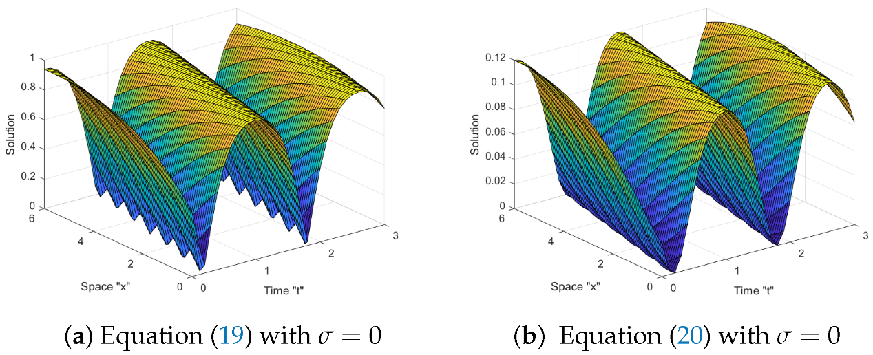
In this article, the impact of noise on the acquired solutions of the SDSEs (1) and (2) is addressed. Depending on the research on the topic [40,41,42,43,44], the stabilizing and destabilizing influences caused by noisy terms in deterministic systems are currently well understood. It is now beyond question that these effects are important for understanding the long-term behavior of actual systems. For various noise strengths $\sigma$, we utilize the MATLAB tools (for more details, see, for example, [45]) to create some figures for some solutions such as (19) and (20). The following parameters are fixed: $\kappa =-1,\delta =i,{\rho }_1={\zeta }_1=0.3,{\rho }_2={\zeta }_2=1$, ${\rho }_3=0.2$ and $y=0.5$. Then, ${\zeta }_3=2.18,{\gamma }_1=\frac{2}{1.09}$ and ${\gamma }_2=\frac{149}{91}$. In this case, $m=0.8$, ${\ell }_1=1.28$ and $\zeta =0.3x+0.5-2.8t.$

In Figure 1, when $\sigma =0,$ we notice that the surface fluctuates.

Meanwhile, in Figure 2, if the intensity of the noise is raised, the surface becomes more planer after small transit behaviors, as follows:

We conclude from the previous figures that the noise term must be included in the Davey–Stewartson Equations (1) and (2) in order to produce accurate results and stable solutions that are near to zero.

5. Conclusions

This work took into account the stochastic (2+1)-dimensional Davey–Stewartson Equations (1) and (2) forced by multiplicative noise. Using the mapping method, we were able to generate stochastic trigonometric, elliptic, hyperbolic and rational solutions. For further study in fields such as hydrodynamics nonlinear optics, plasma physics, and others, the discovered solutions will be very beneficial. Due to the significance of the Davey–Stewartson equations in plasma physics, nonlinear optics, hydrodynamics and other fields, the obtained solutions are useful in explaining a number of intriguing physical phenomena. Additionally, we generalized previously obtained results, such as the one described in [31,37,38]. As a result of our results, we deduced that multiplicative Brownian motion stabilizes the solutions at zero. Finally, a demonstration of how multiplicative Brownian motion influences the exact solutions of the SDSEs is provided. We may take into account the additive noise in future work, as the multiplicative noise was covered in this paper.

References

- Wazwaz, A.M. The tanh method: Exact solutions of the Sine–Gordon and Sinh–Gordon equations. Appl. Math. Comput. 2005, 167, 1196–1210. [Google Scholar] [CrossRef]
- Mohammed, W.W.; Alshammari, M.; Cesarano, C.; El-Morshedy, M. Brownian Motion Effects on the Stabilization of Stochastic Solutions to Fractional Diffusion Equations with Polynomials. Mathematics 2022, 10, 1458. [Google Scholar] [CrossRef]
- Al-Askar, E.M.; Mohammed, W.W.; Albalahi, A.M.; El-Morshedy, M. The Impact of the Wiener process on the analytical solutions of the stochastic (2+1)-dimensional breaking soliton equation by using tanh–coth method. Mathematics 2022, 10, 817. [Google Scholar] [CrossRef]
- Zaman, U.H.M.; Arefin, M.A.; Akbar, M.A.; Uddin, M.H. Analytical behavior of soliton solutions to the couple type fractional-order nonlinear evolution equations utilizing a novel technique. Alex. Eng. J. 2022, 61, 11947–11958. [Google Scholar] [CrossRef]
- Khatun, M.A.; Arefin, M.A.; Islam, M.Z.; Akbar, M.A.; Uddin, M.H. New dynamical soliton propagation of fractional type couple modified equal-width and Boussinesq equations. Alex. Eng. J. 2022, 61, 9949–9963. [Google Scholar] [CrossRef]
- Wazwaz, A.M. An analytic study of compactons structures in a class of nonlinear dispersive equations. Math. Comput. Simul. 2003, 63, 35–44. [Google Scholar] [CrossRef]
- Wen-Xiu, M.; Sumayah, B. A binary darboux transformation for multicomponent NLS equations and their reductions. Anal. Math. Phys. 2021, 11, 44. [Google Scholar]
- Yan, Z.L. Abunbant families of Jacobi elliptic function solutions of the-dimensional integrable Davey-Stewartson-type equation via a new method. Chaos Solitons Fract. 2003, 18, 299–309. [Google Scholar] [CrossRef]
- Fan, E.; Zhang, J. Applications of the Jacobi elliptic function method to special-type nonlinear equations. Phys. Lett. A 2002, 305, 383–392. [Google Scholar] [CrossRef]
- Wazwaz, A.M. A sine-cosine method for handling nonlinear wave equations. Math. Comput. Model. 2004, 40, 499–508. [Google Scholar] [CrossRef]
- Yan, C. A simple transformation for nonlinear waves. Phys. Lett. A 1996, 224, 77–84. [Google Scholar] [CrossRef]
- Wang, M.L.; Li, X.Z.; Zhang, J.L. The (G’/G)-expansion method and travelling wave solutions of nonlinear evolution equations in mathematical physics. Phys. Lett. A 2008, 372, 417–423. [Google Scholar] [CrossRef]
- Zhang, H. New application of the (G’/G)-expansion method. Commun. Nonlinear Sci. Numer. Simul. 2009, 14, 3220–3225. [Google Scholar] [CrossRef]
- Hirota, R. Exact solution of the Korteweg-de Vries equation for multiple collisions of solitons. Phys. Rev. Lett. 1971, 27, 1192–1194. [Google Scholar] [CrossRef]
- Khan, K.; Akbar, M.A. The exp(−(ς))-expansion method for finding travelling wave solutions of Vakhnenko-Parkes equation. Int. J. Dyn. Syst. Differ. Equ. 2014, 5, 72–83. [Google Scholar]
- Mohammed, W.W.; Blömker, D. Fast-Diffusion Limit with Large Noise for Systems of Stochastic Reaction-Diffusion Equations. Stoch. Anal. Appl. 2016, 34, 961–978. [Google Scholar] [CrossRef] [Green Version]
- Mohammed, W.W.; Blömker, D. Fast-diffusion limit for reaction-diffusion equations with multiplicative noise. J. Math. Anal. Appl. 2021, 496, 124808. [Google Scholar] [CrossRef]
- Elbrolosy, M.E.; Elmandouh, A.A. Dynamical behaviour of nondissipative double dispersive microstrain wave in the microstructured solids. Eur. Phys. J. 2021, 136, 955. [Google Scholar] [CrossRef]
- Elmandouha, A.A.; Ibrahim, A.G. Bifurcation and travelling wave solutions for a (2+1)-dimensional KdV equation. J. Taibah Univ. Sci. 2020, 14, 139–147. [Google Scholar] [CrossRef] [Green Version]
- Elmandouha, A.A. Bifurcation and new traveling wave solutions for the 2D Ginzburg–Landau equation. Eur. Phys. Plus 2020, 135, 1–13. [Google Scholar]
- Elbrolosy, M.E.; Elmandouh, A.A. Construction of new traveling wave solutions for the (2+1) dimensional extended kadomtsev-petviashvili equation. J. Appl. Anal. Comput. 2022, 12, 533–550. [Google Scholar] [CrossRef]
- Elmandouh, A.A.; Elbrolosy, M.E. New traveling wave solutions for Gilson–Pickering equation in plasma via bifurcation analysis and direct method. Math. Methods Appl. Sci. 2022, accepted. [Google Scholar] [CrossRef]
- Yang, X.F.; Deng, Z.C.; Wei, Y. A Riccati-Bernoulli sub-ODE method for nonlinear partial differential equations and its application. Adv. Diff. Equa. 2015, 1, 117–133. [Google Scholar] [CrossRef]
- Filiz, A.; Ekici, M. Sonmezoglu A. F-expansion method and new exact solutions of the Schrödinger-KdV equation. Sci. World J. 2014, 2014, 14. [Google Scholar] [CrossRef] [Green Version]
- Arnold, L. Random Dynamical Systems; Springer: Berlin/Heidelberg, Germany, 1998. [Google Scholar]
- Weinan, E.; Li, X.; Vanden-Eijnden, E. Some recent progress in multiscale modeling. In Multiscale Modeling and Simulation; Lecture Notes in Computational Science and Engineering; Springer: Berlin/Heidelberg, Germany, 2004; Volume 39, pp. 3–21. [Google Scholar]
- Mohammed, W.W. Amplitude equation with quintic nonlinearities for the generalized Swift-Hohenberg equation with additive degenerate noise. Adv. Differ. Equ. 2016, 2016, 84. [Google Scholar] [CrossRef] [Green Version]
- Mohammed, W.W.; Iqbal, N.; Botmart, T. Additive noise effects on the stabilization of fractional-space diffusion equation solutions. Mathematics 2020, 10, 130. [Google Scholar] [CrossRef]
- Kloeden, P.E.; Platen, E. Numerical Solution of Stochastic Differential Equations; Springer: New York, NY, USA, 1995. [Google Scholar]
- Davey, A.; Stewartson, K. On three-dimensional packets of surface waves. Proc. Royal. Soc. Lond. Ser. A 1974, 338, 101–110. [Google Scholar]
- Bhrawy, A.H.; Abdelkawy, M.A.; Biswas, A. Cnoidal and snoidal wave solutions to coupled nonlinear wave equations by the extended Jacobi’s elliptic function method. Commun. Nonlinear Sci. Numer. Simul. 2013, 18, 915–925. [Google Scholar] [CrossRef]
- Jafari, H.; Sooraki, A.; Talebi, Y.; Biswas, A. The first integral method and traveling wave solutions to Davey–Stewartson equation. Nonlinear Anal. Model. Control 2012, 17, 182–193. [Google Scholar] [CrossRef] [Green Version]
- Mirzazadeh, M. Soliton solutions of Davey–Stewartson equation by trial equation method and ansatz approach. Nonlinear Dyn. 2015, 82, 1775–1780. [Google Scholar] [CrossRef]
- El Achab, A. Constructing new wave solutions to the (2+1)-dimensional Davey–Stewartson equation (DSE) which arises in fluid dynamics. JMST Adv. 2019, 1, 227–232. [Google Scholar] [CrossRef] [Green Version]
- Fu, H.M.; Dai, Z.D. Double exp-function method and application. Int. J. Nonlinear Sci. Numer. Simul. 2009, 10, 927–933. [Google Scholar] [CrossRef]
- Abdelaziz, M.A.M.; Moussa, A.E.; Alrahal, D.M. Exact Solutions for the nonlinear (2+1)-dimensional Davey-Stewartson equation using the generalized (G’/G)-expansion method. J. Math. Res. 2014, 6, 91–99. [Google Scholar] [CrossRef] [Green Version]
- Ebadi, G.; Biswas, A. The (G’/G) method and 1-soliton solution of the Davey–Stewartson equation. Math. Comput. Model. 2011, 53, 694–698. [Google Scholar] [CrossRef]
- Zedan, H.A.; Monaquel, S.J. The sine-cosine method for the Davey-Stewartson equations. Appl. Math. E-Notes 2010, 10, 103–111. [Google Scholar]
- Peng, Y.Z. Exact solutions for some nonlinear partial differential equations. Phys. Lett. A 2003, 314, 401–408. [Google Scholar] [CrossRef]
- Caraballo, T.; Langa, J.A.; Valero, J. Stabilisation of differential inclusions and PDEs without uniqueness by noise. Commun. Pure Appl. Anal. 2008, 7, 1375–1392. [Google Scholar] [CrossRef]
- Caraballo, T.; Robinson, J.C. Stabilisation of linear PDEs by Stratonovich noise. Syst. Control. Lett. 2004, 53, 41–50. [Google Scholar] [CrossRef] [Green Version]
- Mackey, M.C.; Longtin, A.; Lasota, A. Noise-induced global asymptotic stability. J. Stat. Phys. 1990, 60, 735–751. [Google Scholar] [CrossRef]
- Blömker, D.; Fu, H. The impact of multiplicative noise in SPDEs close to bifurcation via amplitude equations. Nonlinearity 2020, 33, 3905. [Google Scholar] [CrossRef]
- Caraballo, T.; Kloeden, P.E. Stabilization of evolution equations by noise. Interdiscip. Math. Sci. 2009, 8, 43–66. [Google Scholar]
- Higham, D.J. An algorithmic introduction to numerical simulation of stochastic differential equations. SIAM Rev. 2001, 43, 525–546. [Google Scholar] [CrossRef]
Publisher’s Note: MDPI stays neutral with regard to jurisdictional claims in published maps and institutional affiliations. |
© 2022 by the authors. Licensee MDPI, Basel, Switzerland. This article is an open access article distributed under the terms and conditions of the Creative Commons Attribution (CC BY) license (https://creativecommons.org/licenses/by/4.0/).
Share and Cite
MDPI and ACS Style
Al-Askar, F.M.; Cesarano, C.; Mohammed, W.W. Multiplicative Brownian Motion Stabilizes the Exact Stochastic Solutions of the Davey–Stewartson Equations. Symmetry 2022, 14, 2176. https://doi.org/10.3390/sym14102176
AMA Style
Al-Askar FM, Cesarano C, Mohammed WW. Multiplicative Brownian Motion Stabilizes the Exact Stochastic Solutions of the Davey–Stewartson Equations. Symmetry. 2022; 14(10):2176. https://doi.org/10.3390/sym14102176
Chicago/Turabian StyleAl-Askar, Farah M., Clemente Cesarano, and Wael W. Mohammed. 2022. "Multiplicative Brownian Motion Stabilizes the Exact Stochastic Solutions of the Davey–Stewartson Equations" Symmetry 14, no. 10: 2176. https://doi.org/10.3390/sym14102176
Note that from the first issue of 2016, this journal uses article numbers instead of page numbers. See further details here.