Research on Tunnel Construction Monitoring Method Based on 3D Laser Scanning Technology

Abstract

A tunnel is a symmetric structure working under uncertain load. In the traditional method of monitoring and measurement of tunnel deformation, only a small number of symmetric measuring point displacements are engaged to represent the overall deformation of the tunnel, and it is difficult to fully reflect the displacement changes of the tunnel during the construction process. In this paper, a deformation monitoring method is proposed for the tunnel construction process based on 3D laser scanning technology. Initially, 3D laser scanning was used to obtain scattered clouds of irregular structures considering the New Austrian Tunneling Method (NATM). Afterward, the modified B-spline interpolation and greedy triangulation were used to fit the surfaces. Moreover, the normal vector matrix was innovatively applied to express the deformation of the tunnel fitting surface, which solved the problem of scattered point clouds in 3D laser scanning. A normal vector was obtained by the intersection of the normal of one fitted surface with the other. Subsequently, the maximum entropy method was introduced to form the probability density function of the normal vector, and the 1% and 5% probability eigenvalues were used to analyze the overall deformation trend of the tunnel. Finally, the eigenvalue of 5% probability, which was less affected by construction uncertainties, was selected for analysis. This way, the analysis and prediction method for overall tunnel deformation was established.

1. Introduction

Tunnels are symmetric structures working under uncertain loads. The concept of the New Austrian Tunneling Method (NATM) was proposed in the 1960s, and it is still considered to be a basic method for tunnel construction in weak and broken surrounding rock areas. Its core principle is to apply a thin layer of flexible shotcrete and bolt support close to the surrounding rock near the excavation surface to control the deformation and stress release of the surrounding rock. To implement the dynamic design of the tunnel, NATM requires vigilant tunnel monitoring and measurement, which are crucial tools for controlling deformation.

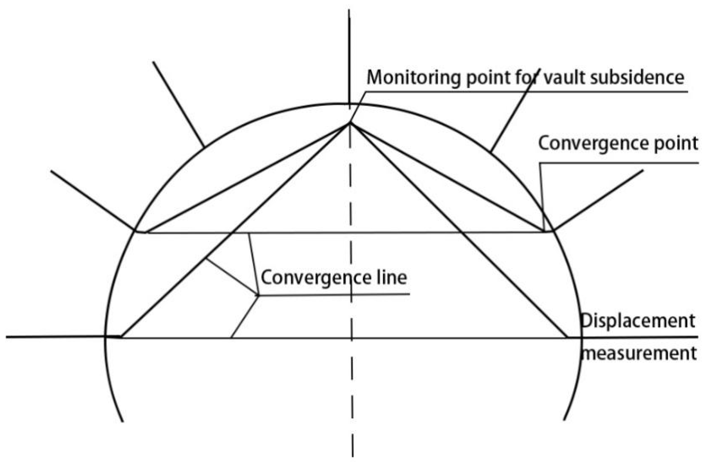
Monitoring and measurement of the stability and deformation of the surrounding rock, surface, and supporting structure are critical to collecting necessary data during tunnel construction. On-site measurements of the surrounding rock can be used to monitor the structural response, evaluate the structural safety in real-time, maintain structure safety and symmetry in nature [1], determine the timing of secondary lining, substantiate the rationality of the selected support method, and guide the design and construction of tunnels [2]. As shown in Figure 1, traditional monitoring and measurement use indices such as vault subsidence and convergence deformation [3] to characterize the deformation of the surrounding rock of the tunnel. Currently, monitoring and measurement are usually carried out using a total station, with reflective signs at the measuring points. However, this method has four shortcomings: the small number of measuring points makes it impossible to prevent the issue of falling blocks of the vault; the deformation of the biased tunnel measuring points is insufficiently representative [4], which distorts monitoring and measurement results; blasting construction damage and pollution reflective signs result in invalidation of monitoring and measurement outcomes; and the monitoring and measurement process takes a long time, which impacts the safety and health of the inspectors and hinders the normal construction process [5].

Three-dimensional laser scanning technology uses the principle of laser ranging to make a contactless measurement and can directly obtain massive 3D point clouds with irregular spatial distribution that can be used in reverse engineering [6]. Additionally, it has a certain degree of penetrability and is less affected by the environment. It has played an increasingly important role in global change, smart cities, resource surveys, environmental monitoring, basic mapping, and other pertinent fields [7,8,9].

Three-dimensional laser scanning technology has been gradually employed in tunnel construction owing to its fast detection speed, large quantity, high level of automation, strong environmental adaptability, and good adaptability to tunnel deformation measurement. Further, it allows for a comparison between the point cloud or the fitted point cloud surface with the design surface and helps in detecting the over-excavation and under-excavation of the tunnel [10]. Three-dimensional laser scanning technology has been widely used in the construction and operation of shield tunnels. The overall procedure of tunnel deformation using this technology includes the projection of the point cloud on the tunnel section, fitting the 3D laser scanner into the tunnel outline, calculating the vertical and horizontal diameters, and judging the tunnel deformation through the change in ellipticity [11]. The geometric information of the tunnel is contained in the detected point cloud during tunnel construction as per NATM, and this technology is also being adopted gradually for the detection of over- and under-excavation of tunnels. The tunnel point cloud is analyzed and studied using direct graphic comparison [12]. However, 3D laser scanning technology is rarely used in tunnel monitoring and measurement schemes. Therefore, this paper focuses on solving two major obstacles, i.e., the comparison of randomly distributed point clouds and the denoising of abnormal points. Additionally, considering that 3D laser scanning technology is an important means of reverse engineering, this paper employs the cloud platform to collect data and self-compiled software for analysis and processing.

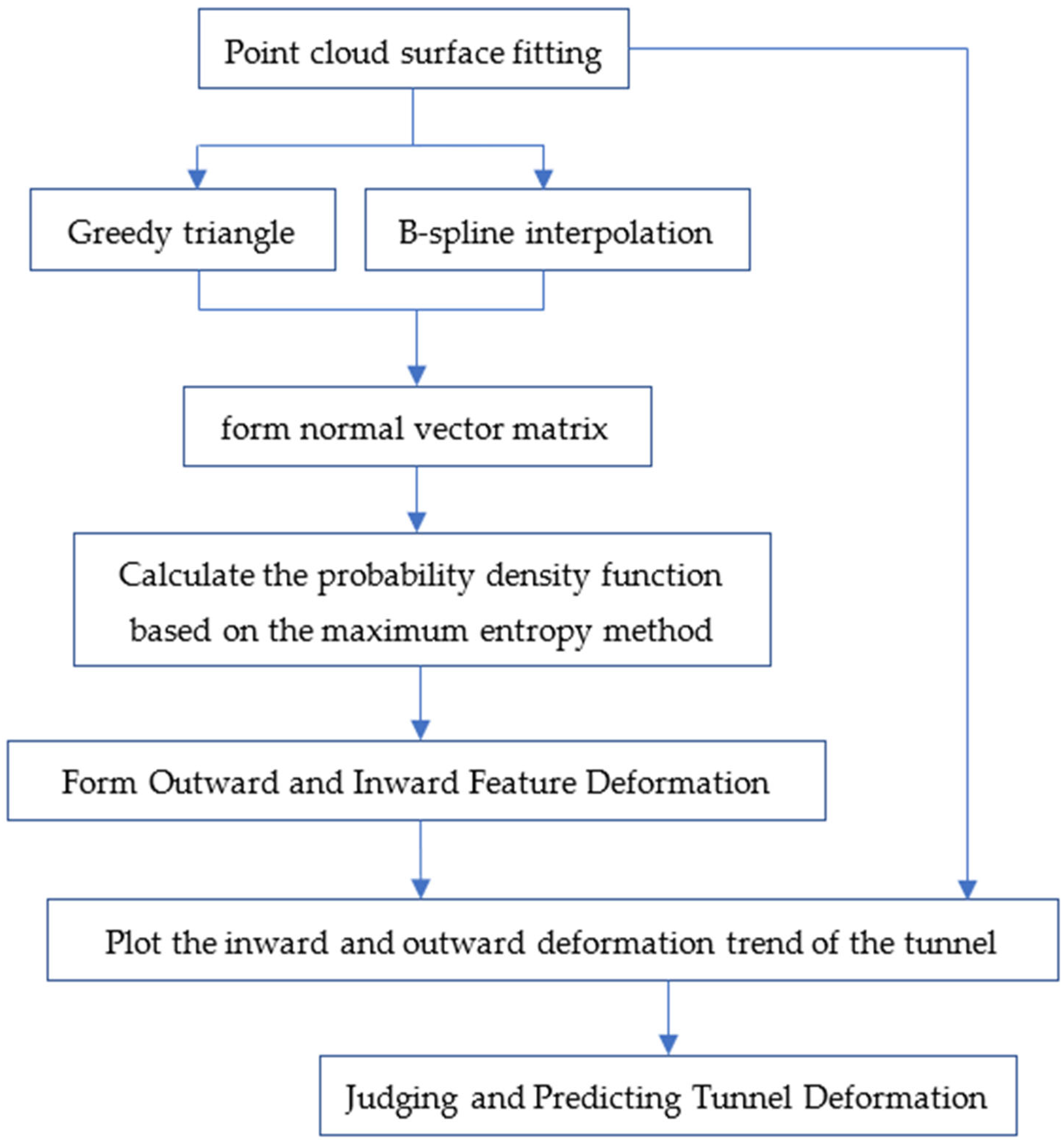
In order to solve the analysis problem of the scattered point cloud, B-spline interpolation and a greedy triangulation were used to fit the tunnel surfaces. Afterward, the surfaces of the tunnel were compared before and after the measurement. This paper innovatively used the method of forming a normal vector matrix for comparison and introduced the maximum entropy method to create the probability density function of the normal vector and extract the deformation eigenvalues. The deformation eigenvalues were then used to create a curve that could assess and forecast tunnel deformation. The flowchart is shown in Figure 2.

2. Fitting Surface

Surface fitting is the basis for conducting scattered point cloud analysis, whereas scattered point clouds cannot be compared. After the curved surface is fitted, the comparison between the curved surfaces can be realized to understand the deformation of the tunnel.

Surface fitting of a point cloud is the process of fitting a discrete point cloud onto a surface for general analysis. The accuracy of the surface fitting has direct implications for the calculation outcomes [13]. The degree of fitting optimization can be effectively improved by selecting the right fitting method to obtain the reference surface for flatness calculation. The choice of an appropriate fitting model is crucial for surface fitting because it has a direct impact on the precision of parameter solution and surface fitting in the subsequent data processing.

2.1. Bicubic Spline Interpolation Surface Construction

The cubic B-spline interpolation method is the process of obtaining a curve function group by mathematically solving the three bending moment equations through a smooth curve having a series of shape value points.

In the 2D plane curve interpolation, the cubic spline function on nodes x₀, x₁, ..., x_n is defined as $S(x)\in C2[a,b]$; it is a cubic polynomial in each small interval $[x_j,x_{j+1}]$, where $a=x_0<x_1<\cdots <x_n=b$ defines subjected node. If the function value $Y_j=f(X_j)(j=0,1,\cdots ,n)$ is given on the node x_j, and the cubic spline function is established as $S(x_j)=y_j(j=0,1,\cdots ,n)$, then $S(x)$ is referred to as the cubic spline interpolation function.

For m + n + 1 scattered points in the space, the surface is solved by the point cloud composed of scattered points; ${\mathrm{Q}}_h(h=0,1,2,\dots ,m+n)$ represents the set of these scattered points. Thus the n-th spline curve can be defined as follows [14]:

$$Q_{i,n}(t)={\displaystyle \sum _{k=0}^n{Q}_{i+k}}{Y}_{k,n}(t)$$

(1)

where $Y_{k,n}(t)$ is the basic function of the n-th degree spline function, and t represents the node parameter, i.e., $t\in \left[0,1\right]$.

In spline interpolation, when n = 3 and k = 0, 1, 2, 3, the polygon can be represented by 4 points, i.e., $Q_0,Q_1,Q_2,Q_3$. The cubic spline is a cubic polynomial defined as follows [15]:

$$Y_{0,3}(t)=\frac{1}{6}(-t^3+3t^2-3t+1)$$

(2)

$$Y_{1,3}(t)=\frac{1}{6}(3t^3-6t^2+4)$$

(3)

$$Y_{2,3}(t)=\frac{1}{6}(-3t^3+3t^2+3t+1)$$

(4)

$$Y_{3,3}(t)=\frac{1}{6}{t}^3$$

(5)

Thus, the expression of the cubic spline is:

$$Q_{i,3}(t)={\displaystyle \sum _{k=0}^3{Q}_{i+k}}{Y}_{k,3}(t)=Q_i{Y}_{0,3}(t)+Q_{i+1}{Y}_{1,3}(t)+Q_{i+2}{Y}_{2,3}(t)+Q_{i+3}{Y}_{3,3}(t)$$

(6)

where $i=0,1,2,\dots ,m$.

Following the principle of cubic spline interpolation in 2D space, a method is introduced for 3D space to obtain the interpolation surface of the bicubic spline. For this purpose, considering the n × m-th degree parametric surface as the calculation surface and (n + 1) × (m + 1) scattered points in the space, the multi-degree polynomial composed of i and j can be used for the solution, which can be solved in the form of a matrix. The space grid is formed by connecting two adjacent points in the point set with line segments, which is used as the control network and can be defined as follows.

$$Q(u,v)={\displaystyle \sum _{i=0}^n{\displaystyle \sum _{j=0}^m{Q}_{ij}}}{Y}_{in}(u)Y_{jm}(v)$$

(7)

where $Q_{ij}$ is the control vertex of the surface, u and v represent parameters in two directions, i.e., 0 ≤ u ≤ 1 and 0 ≤ v ≤ 1; $Y_{in}(u)$ and $Y_{jm}(v)$ represent the spline-based functions in u and v directions on the plane coordinates. The characteristic mesh of the bicubic B-spline surface is formed when m = n = 3, and the equation of the bicubic B-spline surface can be given as follows:

$$Q\left(u,v\right)=U{B}_{3}Q{B}_3^T{V}^T$$

(8)

where $U=\left[\begin{array}{cccc}{u}^3& u^2& u& 1\end{array}\right]$, $V=\left[\begin{array}{cccc}{v}^3& v^2& v& 1\end{array}\right]$.

$$B=\frac{1}{6}\left[\begin{array}{cccc}-1& 3& -3& 1\\ 3& -6& 3& 0\\ -3& 0& 3& 0\\ 1& 4& 1& 0\end{array}\right]$$

(9)

$$Q=\left[\begin{array}{cccc}{Q}_{i,j}& Q_{i,j+1}& Q_{i,j+2}& Q_{i,j+3}\\ Q_{i+1,j}& Q_{i+1,j+1}& Q_{i+1,j+2}& Q_{i+1,j+3}\\ Q_{i+2,j}& Q_{i+2,j+1}& Q_{i+2,j+2}& Q_{i+2,j+3}\\ R_{i+3,j}& R_{i+3,j+1}& R_{i+3,j+2}& R_{i+3,j+3}\end{array}\right]$$

(10)

2.2. Greedy Projection Triangulation Algorithm

The Delaunay triangulation method is tedious and difficult to converge. The greedy algorithm does not consider the overall situation, and it only seeks the local optimal solution [16,17,18]. Therefore, in the point cloud fitting, the greedy algorithm is considered a local fitting method. On the other hand, the number of point clouds is extremely large; therefore, the greedy algorithm eliminates the need to exhaust all possibilities to find the optimal solution and requires extensive computing time. For each point cloud subset, the problem is divided into smaller subsets, and the best fitting results from those subsets are used, since the greedy algorithm is capable of obtaining the local optimal result. Given that the correlation between the point clouds is not very high, the greedy algorithm is feasible for fitting the 3D laser scanning point clouds.

Greedy projection triangulation involves projecting the point cloud from the point cloud subset into a plane along the normal direction of the point cloud data and then triangulating to determine the topological relationship of each point using the Delaunay triangulation method [19,20]. By selecting a sample triangle as the initial surface, the boundary of the surface is continuously expanded and extended until all the points that are geometrically and topologically correct are connected. This way, a complete triangular mesh surface is formed. The specific steps are as follows [21]:

• The KD tree structure is used to determine the nearest points; this step is called nearest neighbor search.
• The plane and the surface are made roughly tangential to project the point cloud’s normal information to the plane in blocks.
• The procedure is completed by projecting the points to the plane, triangulating the points on the plane, reflecting the topological relationship into the space, and concluding the continuous cycle of surface reconstruction.

2.3. Ablation Study

• The point cloud and surface are compatible with the greedy triangulation method, which can accurately express the tunnel’s local surface. When the density of the point cloud is high, the effect of the abrupt change in the normal angle can be overlooked because of the small change in the normal angle between adjacent triangles. A major surface fitting method for 3D laser scanning monitoring and measurement can be used in future research, given the high acceptance of this method in the engineering field.
• The B-spline interpolation method can restore the tunnel girdle area with minimal curvature by fitting the tunnel face with a polynomial in the whole area. At the same time, it maintains high goodness of fit. However, the fitting surface of the vault (area with large curvature) has a distorted position, and the partition fitting method is used to improve the fitting degree. The normal angle is continuously changing; the fitting surface is smooth and continuous at high orders. However, the fitting surface does not tend to overlap with the point cloud and has a tendency to disregard the local variations of the tunnel. Therefore, engineers and technicians have a low level of acceptance for this method; thus, it can be used as an auxiliary fitting method in future studies and compared to the greedy triangulation method for validation.

3. Deformation Hypothesis

A full-fitting surface is created after tunnel fitting. However, since point clouds cannot be tracked by 3D laser scanners, the authors were unable to determine the direction in which each point in the tunnel was moved. The initial support surface of the tunnel is also quite complicated, which seriously affects the monitoring and measurement of the tunnel.

The tunnel comprises the surrounding rock and initial support to form an arched structure. The arched structure is a compression bending member or an axial compression member. Compressive instability failure features of the tunnel arch ring under pressure are seen in the case of the original support of the tunnel being destroyed. Therefore, it is assumed that the deformation direction of the initial support surface of the tunnel is in the normal direction of the fitted surface. According to the traditional monitoring and measurement method, the monitoring of vault settlement and peripheral convergence also aligns with the assumption that the tunnel is deformed along the normal direction. In order to determine the process of tunnel deformation, make predictions of deformation and realize early warnings of tunnel arch bridge instability, this article compares and analyzes the two-point cloud fitting surfaces before and after using the normal vector.

4. Monitoring and Measurement Algorithm Based on Scattered Point Cloud

4.1. Observation Point Arrangement of the Fitting Surface

Cloud data of 3D laser scanning are discrete and randomly distributed and require a continuous function model [22]. Therefore, the point cloud data of the initial support of the tunnel detected each time are fitted to obtain the fitting surface function of the point cloud, i.e., $S=f(x,y,z)$. In order to simplify the calculation, the point cloud data are selected at preset time intervals, and the first, second and nth data fitting surfaces are set as $S_1=f_1(x,y,z)$, $S_2=f_2(x,y,z)$ and $S_n=f_n(x,y,z)$, respectively.

According to the same circumferential angle and longitudinal distance, the points are arranged on the curved surface of the previous tunnel fitting as the monitoring points for monitoring and measurement. This ensures the uniform arrangement of the tunnel surface points on the plane composed of the tunnel central axis and the tunnel vault axis. The observation points needed for monitoring and measuring are uniformly distributed and are assigned to matrix A in the point set, as follows.

$$\mathrm{A}=\left[\begin{array}{cccc}{a}_{1,1}& a_{1,2}& \dots \dots & a_{1,j}\\ a_{2,1}& a_{2,2}& \dots \dots & a_{2,j}\\ ·& ·& ·& ·\\ ·& ·& ·& ·\\ ·& ·& ·& ·\\ a_{i,1}& a_{i,2}& \dots \dots & a_{i,j}\end{array}\right]$$

(11)

4.2. Calculation of Initial Support Deformation of Tunnel

Starting from the observation point matrix B and assuming that the initial support of the tunnel only creates displacement in the normal direction, the normal of the first data fitting surface, $S_1=f_1(x,y,z)$, is determined. Based on the partial derivative of the binary function, the partial derivative at the point (x₀, y₀) can be given as follows:

$$f{’}_{\mathrm{x}}(x_0,y_0)=\underset{\Delta x\to 0}{{\displaystyle \lim }}\frac{f(x_0+\Delta x,y_0)-f(x_0,y_0)}{\Delta x}$$

(12)

$$f{’}_{\mathrm{y}}(x_0,y_0)=\underset{\Delta \mathrm{y}\to 0}{{\displaystyle \lim }}\frac{f(x_0,y_0+\Delta \mathrm{y})-f(x_0,y_0)}{\Delta \mathrm{y}}$$

(13)

Further, the first data fitting surface $S_1=f_1(x,y,z)$ is an implicit function, i.e., F(x, y, z), which implies that

$$\frac{\partial \mathrm{z}}{\partial \mathrm{x}}=-\frac{F{’}_x(x,y,z)}{F{’}_z(x,y,z)}$$

(14)

$$\frac{\partial \mathrm{z}}{\partial \mathrm{y}}=-\frac{F{’}_y(x,y,z)}{F{’}_z(x,y,z)}$$

(15)

Thus, the normal equation for the observation point $a_{\mathrm{i},\mathrm{j}}(x_0,y_0)$ on the first data fitting surface $S_1=f_1(x,y,z)$ can be given as follows:

$$\frac{x-x_0}{{\mathrm{S}}_0{’}_x\left(x_0,y_0,z_0\right)}=\frac{y-y_0}{{\mathrm{S}}_0{’}_y\left(x_0,y_0,z_0\right)}=\frac{z-z_0}{{\mathrm{S}}_0{’}_z\left(x_0,y_0,z_0\right)}$$

(16)

The observation point is based on the normal $f_{i,j}$ of the first data fitting surface; thus, the normal matrix, F, is the absolute value matrix of the normal vector starting from the point $a_{\mathrm{i},\mathrm{j}}$ as follows:

$$\mathrm{F}=\left[\begin{array}{cccc}{f}_{1,1}& f_{1,2}& \dots \dots & f_{1,j}\\ f_{2,1}& f_{2,2}& \dots \dots & f_{2,j}\\ ·& ·& ·& ·\\ ·& ·& ·& ·\\ ·& ·& ·& ·\\ f_{i,1}& f_{i,2}& \dots \dots & f_{i,j}\end{array}\right]$$

(17)

Moreover, matrix B is defined as the set of intersections between the normal and the two curved $S_{\mathrm{n}}=f_{\mathrm{n}}(x,y,z)$ surfaces in the following equation; the distance from A to B can be roughly calculated as the deformation of the initial support of the tunnel.

$$\mathrm{B}=\left[\begin{array}{cccc}{b}_{1,1}& b_{1,2}& \dots \dots & b_{1,j}\\ b_{2,1}& b_{2,2}& \dots \dots & b_{2,j}\\ ·& ·& ·& ·\\ ·& ·& ·& ·\\ ·& ·& ·& ·\\ b_{i,1}& b_{i,2}& \dots \dots & b_{i,j}\end{array}\right]$$

(18)

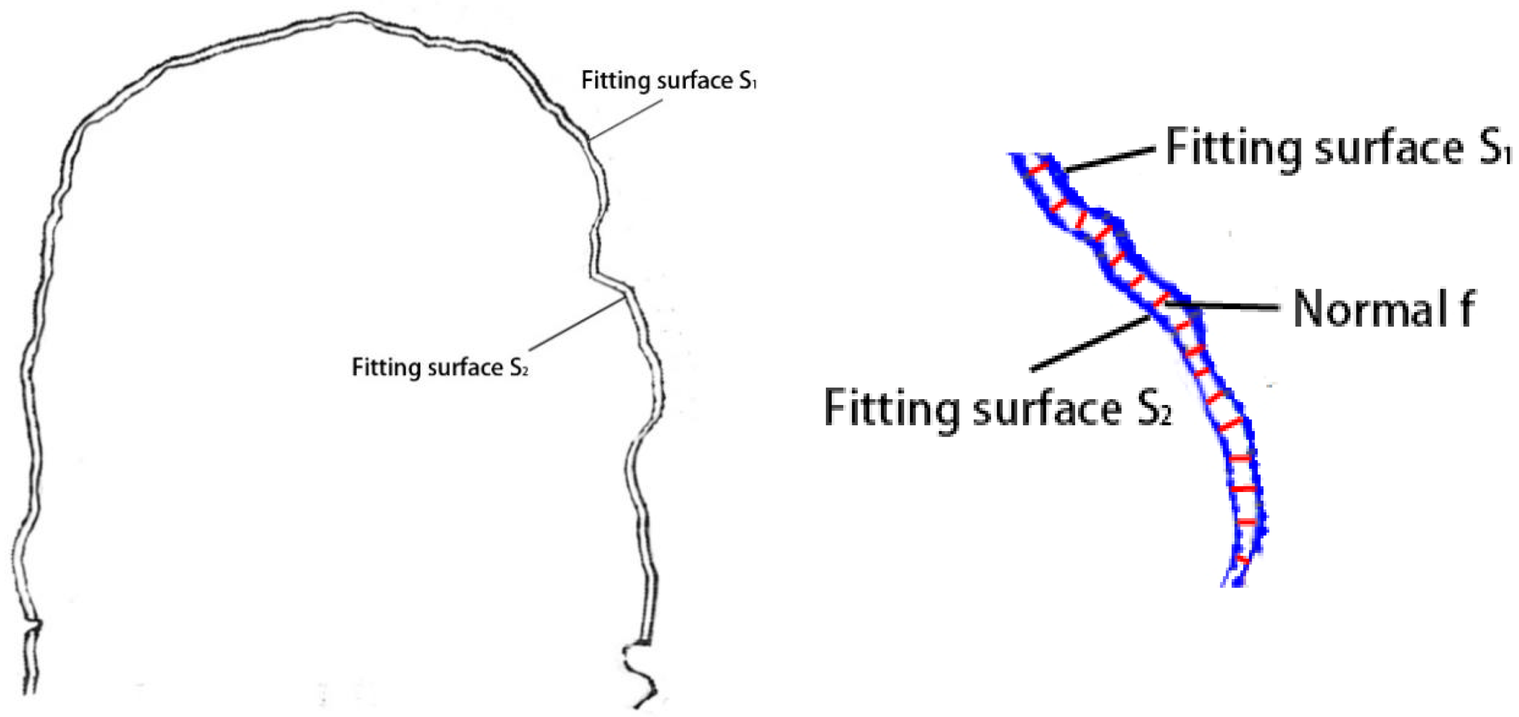
As shown in Figure 3, the tunnel deformation length is the distance between the normal line and the intersection points of $S_1=f_1(x,y,z)$ and $S_{\mathrm{n}}=f_{\mathrm{n}}(x,y,z)$ surfaces. The displacement of S_n is set to be positive when S_n is inside S₁, and negative when S_n is outside S₁. The normal vector matrix D is formed by summarizing the observation points of the displacement.

$$\mathrm{D}=\left[\begin{array}{cccc}{d}_{1,1}& d_{1,2}& \dots \dots & d_{1,j}\\ d_{2,1}& d_{2,2}& \dots \dots & d_{2,j}\\ ·& ·& ·& ·\\ ·& ·& ·& ·\\ ·& ·& ·& ·\\ d_{i,1}& d_{i,2}& \dots \dots & d_{i,j}\end{array}\right]$$

(19)

where

$$\left|\mathrm{d}\right|=\sqrt{{\left(x_{\mathrm{n}}-x_1\right)}^2+{\left(y_{\mathrm{n}}-y_1\right)}^2+{\left(z_{\mathrm{n}}-z_1\right)}^2}$$

(20)

5. Maximum Entropy Analysis of Tunnel Deformation

Maximum Entropy Analysis

Entropy S(x) is used to quantitatively describe the uncertainty or information content of random events or variables [23,24]. The principle of maximum entropy [9] refers to that among all the many probability density functions that satisfy the given constraints; the probability density function with the largest information entropy is considered to be the best (i.e., has the smallest deviation) [25,26,27].

$$\mathrm{S}(x)=-{\displaystyle \sum _{x\in (0,N)}p(x)\ln (p(x))}$$

(21)

where $p(x_i)$ is the probability against the random variable value $x_i$, and N is the number of samples.

When x is a continuous random variable, entropy can be defined by the following Equation:

$$\mathrm{S}(x)=-{\displaystyle {\int }_{-\infty }^{\infty }f(x)\ln f(x)dx}$$

(22)

where $f(x)$ is the probability density function of the random variable distribution.

The following conditions are satisfied considering the normal vector of each observation point of the tunnel $\Delta$ as a continuous random variable and the probability density function $f(\Delta )$ as a function of it.

$$k_0(\Delta )={\displaystyle {\int }_{-\infty }^{+\infty }f(\Delta )d\Delta }-1=0$$

(23)

$$k_i(\Delta )={\displaystyle {\int }_{-\infty }^{+\infty }{\Delta }^{i}f(\Delta )d\Delta }-n_i=0$$

(24)

where $n_i$ is the i-th order origin moment of the statistical sample of $\Delta$, which can be determined by the calculation of the statistical sample.

In order to realize the entropy of the $\Delta$(i.e., $Y(\Delta )$) for the maximum value under the conditions of Equations (23) and (24), the following equation can be specially derived, which is referred to as Lagrange’s Equations (26) and (27):

$$F(\Delta )=Y(\Delta )+{\beta }_0{k}_0(\Delta )+{\displaystyle \sum _{i=1}^N{\beta }_i{k}_i(\Delta )}$$

(25)

where ${\beta }_0,{\beta }_1,{\beta }_2,\cdots ,{\beta }_N$ is the Lagrange multiplier series.

When $\frac{\partial F(\Delta )}{\partial f(\Delta )}=0$, the entropy $Y(\Delta )$ reaches the maximum value, which implies that the following condition is satisfied:

$$\ln f(\Delta )-{\beta }_0-{\displaystyle \sum _{i=1}^N{\beta }_i{\Delta }^i}=0$$

(26)

Thus, the probability density function of the normal vector $\Delta$ of the tunnel observation point represented by the maximum entropy theory can be obtained as follows:

$$f(\Delta )=\exp ({\beta }_0+{\displaystyle \sum _{i=1}^N{\beta }_i{\Delta }^i})$$

(27)

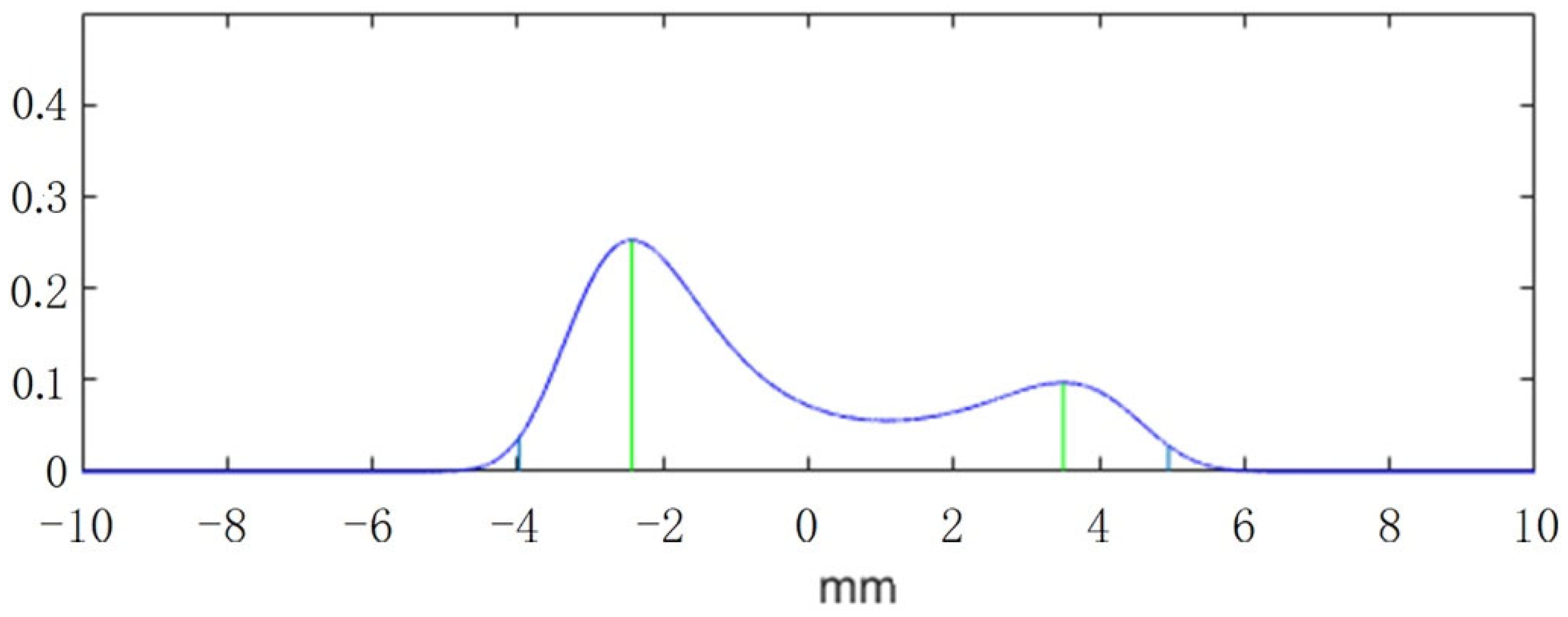
The undetermined coefficients ${\beta }_0,{\beta }_1,{\beta }_2,\cdots ,{\beta }_N$ can be solved by the i+1-element i-th degree equation system using Equations (23) and (24). The probability density function of the normal vector of the tunnel observation point is shown in Figure 4. To improve the convergence of the calculation, this paper adopts the fourth-order moment of the maximum entropy method (i.e., N = 4) [28,29,30,31,32]. This can yield the peak value and position of the probability density function and the characteristic deformation value corresponding to a given set exceedance probability.

This paper uses the ±1% probability feature deformation value in the probability density function of the initial support normal vector of the tunnel as the characteristic deformation value of the tunnel monitoring and measurement analysis. In addition, it takes the ±5% probability feature deformation values for the auxiliary analysis [33,34,35]. Employing the maximum entropy approach’s fourth moment may fully extract sample information generated using this method. Thus, Equations (23) and (24) can yield the following results:

$${\displaystyle {\int }_{{\mathrm{x}}_1}^{+\infty }f({\Delta }_1)d{\Delta }_1}=0.01\left(0.05\right)$$

(28)

$${\displaystyle {\int }_{-\infty }^{{\mathrm{x}}_2}f({\Delta }_2)d{\Delta }_2}=0.01\left(0.05\right)$$

(29)

where ${\Delta }_1$ and ${\Delta }_2$ can be used as the characteristic deformation value of tunnel monitoring and measurement. Considering that the deformation values are mostly concentrated in the peak probability density function, the deformation values ${\Delta }_{1\max }$ and ${\Delta }_{2\max }$ can be used as reference indicators for tunnel monitoring and measurement.

6. Example Verification

In this paper, two sets of point cloud data measured in a railway tunnel were fitted, and the normal vector matrix of the fitted surface was obtained by the method discussed in Section 3. This paper used the maximum entropy method to analyze and process the normal vector probability density function. The fitting methods involved greedy triangulation and B-spline interpolation approaches.

6.1. 3D Laser Scanning Inspection and Deterministic Analysis of Traditional Monitoring Quantity

Considering that the spline interpolation method surface is relatively continuous and stable, and the influence of accidental deformation such as debris interference and blasting damage in the tunnel can be excluded [36,37], the deformation direction is compared using the traditional monitoring and measurement method and the B-spline interpolation method. The monitoring and measuring parts of two traditional techniques in the laser scanning interval, No. 01 and No. 02, were chosen for this study.

Table 1. The traditional monitoring and measurement results for the tunnel (unit: mm).

Compare Dates		14–15	15–16	16–18	18–19	19–21	21–22
Section 01	Vault sinks	17.2	−17.2	10.5	6.0	−7.3	−3.5
	Deformation of the left arch	16.2	−12.0	−7.8	1.7	2.9	2.9
	Deformation of the right arch	−9.5	9.0	−5.6	−4.2	−1.9	−1.8
Section 02	Vault sinks	−24.5	−18.3	−10.2	5.1	−1.7	2.6
	Deformation of the left arch	24.4	−24.4	20.3	−7.2	7.7	2.1
	Deformation of the right arch	−22.8	24.1	−14.5	−3.6	−4.0	−3.1
Maximum forward deformation		24.4	24.1	20.3	6.0	7.7	2.9
Negative deformation maximum		−24.5	−24.4	−14.5	−7.2	−7.3	−3.5

shows differences in the deformation direction of the vault area during the same period using the traditional monitoring method. This phenomenon is also established in the 3D laser scanning detection results. Figure 5 presents the 3D laser scanning inspection, from which it can be interpreted that the deformations of the vault and the arch foot are more complicated, and the positive and negative deformations appear alternately, which is also substantiated by the deformation data of the 14th–15th days in Table 1. The comparison demonstrates that both approaches reflect the same tunnel deformation. On the other hand, the traditional monitoring method employs section deformation judgment, which is incomplete. Three dimensional laser scanning can thoroughly exhibit the deformation, which is more suitable for correct judgment.

Construction records indicate that local blasting was carried out at the under-excavated position on the left side of the tunnel on the 15th–17th days. It can be seen from Table 1 that the overall displacement of the tunnel to the left occurred due to the local blasting. In Figure 6, the yellow area of the tunnel indicates the deformation area to the outside of the tunnel, and the red area indicates the deformation to the inside of the tunnel. During this period, there was a noticeable displacement to the left, and it can be recognized qualitatively that the displacement direction detected by traditional monitoring was fundamentally consistent with the deformation direction acquired by 3D laser scanning detection analysis.

6.2. Quantitative Comparison between 3D Laser Scanning Inspection and Traditional Monitoring Methods

Table 2. Probability feature deformation value of normal vector (unit: mm).

Compare Dates		14–15	15–17	17–18	18–19	19–20	20–21	21–22	22–23
Greedy Triangulation	Positive 1% probability feature deformation value	13.50	12.58	11.70	14.64	13.77	9.12	8.38	-
	Negative 1% probability feature deformation value	−13.51	−12.60	−11.70	−14.63	−13.82	−9.12	−8.38	-
B-spline Interpolation	Positive 1% probability feature deformation value	13.50	19.85	11.69	15.48	11.30	3.41	4.35	-
	Negative 1% probability feature deformation value	−13.49	−15.39	−10.92	−14.28	−14.50	−7.85	−5.38	-
Greedy Triangulation	Positive 5% probability feature deformation value	9.50	8.86	8.18	10.18	9.69	6.43	5.91	-
	Negative 5% probability feature deformation value	−9.50	−8.72	−8.17	−10.20	−9.55	−6.43	−5.91	-
B-spline Interpolation	Positive 5% probability feature deformation value	9.50	12.91	8.11	10.69	8.33	1.93	3.04	-
	Negative 5% probability feature deformation value	−9.50	−11.35	−7.82	−10.24	−9.46	−6.00	−3.82	-

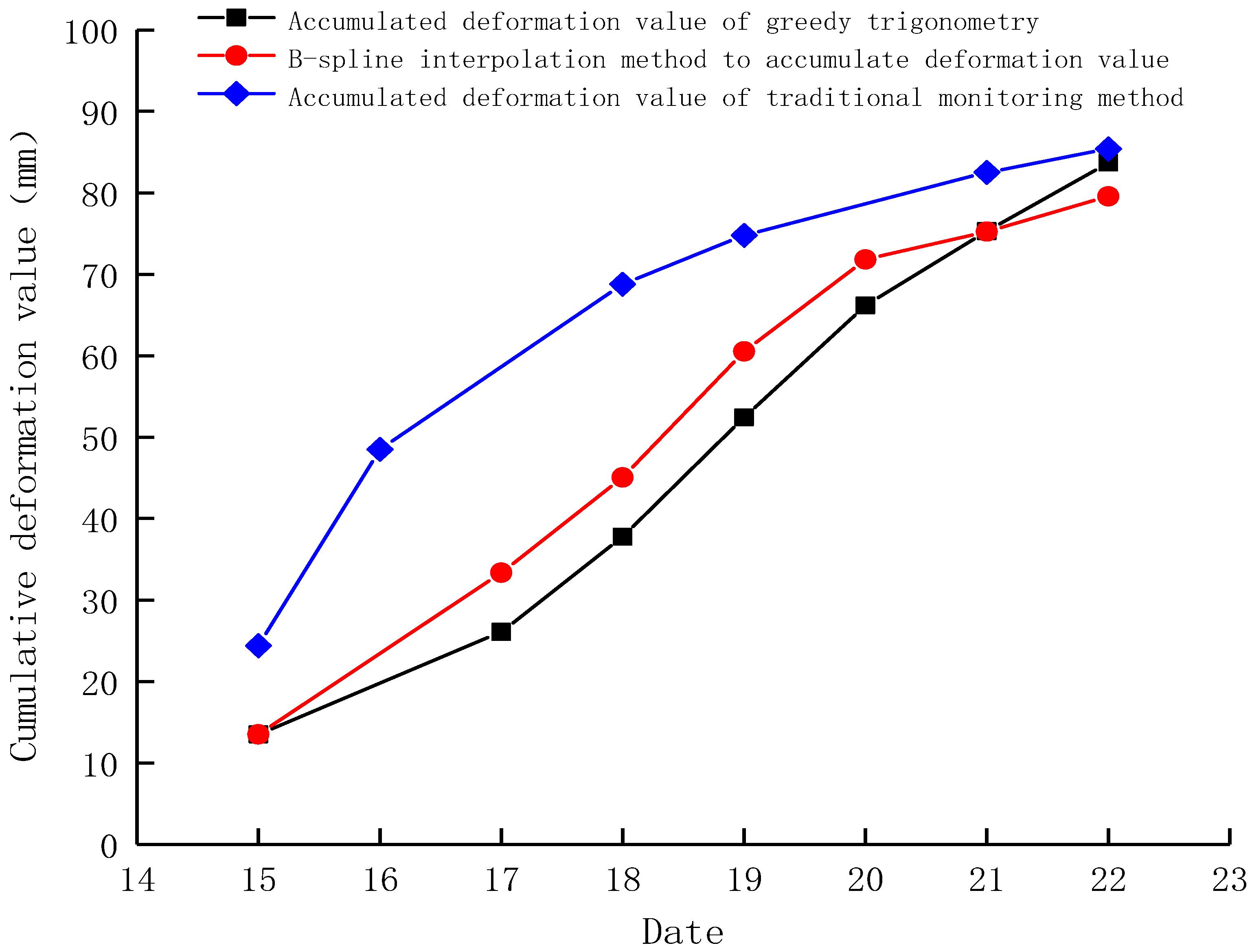
Note: “-” indicates that the overall displacement is small, the data are concentrated, and the calculation is difficult to converge.

compares the characteristic deformation values of the normal vector probability density function of 1% and 5% probability for the greedy triangulation and B-spline interpolation methods. It can be observed that the positive deformation (deformation to the outside of the tunnel) obtained by the B-spline interpolation method was significantly larger on the 15th–17th days and significantly smaller on the 20th−21st days. However, when the data were sufficiently concentrated, the computation did not converge on the 22nd–23rd days while utilizing the maximum entropy approach for data analysis.

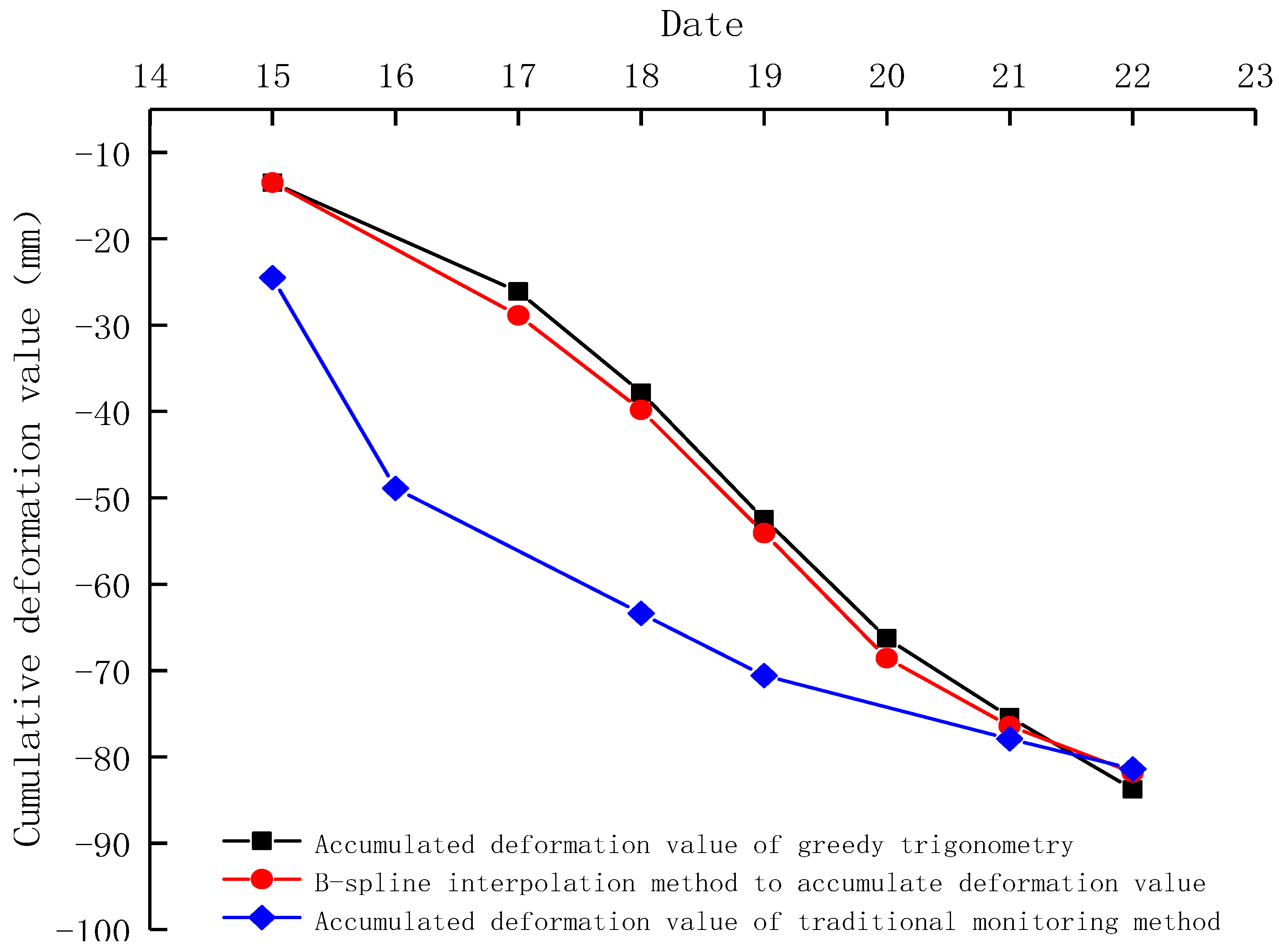
Moreover, observations could not be made by 3D laser scanning on the 16th day and traditional monitoring on the 17th–20th days due to construction interference in the tunnel [38]. Figure 7 and Figure 8 compare the trend of the characteristic deformation value of the 1% probability feature deformation value of the 3D laser scanning with the deformation value measured by traditional monitoring. The 3D laser scanning point cloud adapted well to the greedy triangulation and B-spline interpolation methods for surface fitting.

It can be seen from Figure 7 and Figure 8 that the overall observation trend of the traditional monitoring method and 3D laser scanning were consistent with each other. However, 3D laser scanning yielded more conservative results than the traditional monitoring method. Given the presence of steel arches in the tunnel’s first support, the surrounding rock deformation was not necessarily coordinated with the deformation of the initial support. In addition, it can be observed that the analysis results of the surface fitted by the greedy triangulation method and the surface fitted by the B-spline interpolation method were consistent with marginal deviations at some points.

6.3. Exceedance Probability Characteristic Deformation Value Analysis

In this paper, the gradient change of probability feature deformation value, K_n, was used to validate the results obtained by the greedy triangulation and the B-spline interpolation methods, as follows.

$$K_n=(S_{n+1}-S_n)/S_{n-1}$$

(30)

where S_n is the probability feature deformation value of the specific transcendence probability on an nth day.

Table 3. Comparison of K_n by greedy triangulation and B-spline interpolation method.

Compare Dates		14–15–17	15–17–18	17–18–19	18–19–20	19–20–21	20–21–22
Greedy Triangulation	Negative 1% probability feature deformation value	−7.31%	−7.52%	20.08%	−6.32%	−50.99%	−8.83%
	Positive 1% probability feature deformation value	−7.22%	−7.69%	20.03%	−5.86%	−51.54%	−8.83%
B-spline interpolation	Negative 1% probability feature deformation value	31.99%	−69.80%	24.48%	−36.99%	−231.38%	21.61%
	Positive 1% probability feature deformation value	12.35%	−40.93%	23.53%	1.52%	−84.71%	−45.91%
Greedy Triangulation	Negative 5% probability feature deformation value	−7.22%	−8.31%	19.65%	−5.06%	−50.70%	−8.80%
	Positive 5% probability feature deformation value	−8.94%	−6.73%	19.90%	−6.81%	−48.52%	−8.80%
B-spline interpolation	Negative 5% probability feature deformation value	26.41%	−59.19%	24.13%	−28.33%	−331.61%	36.51%
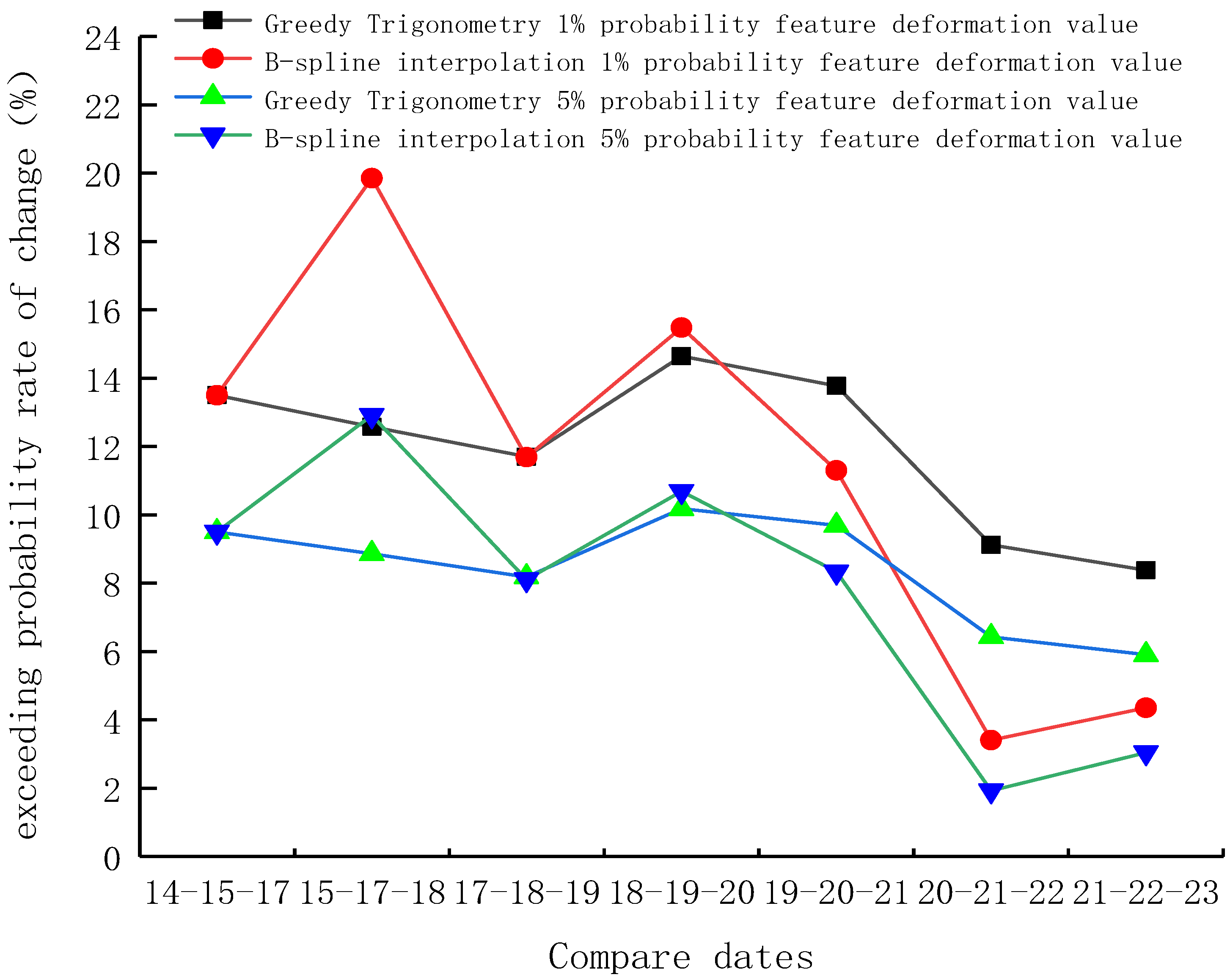
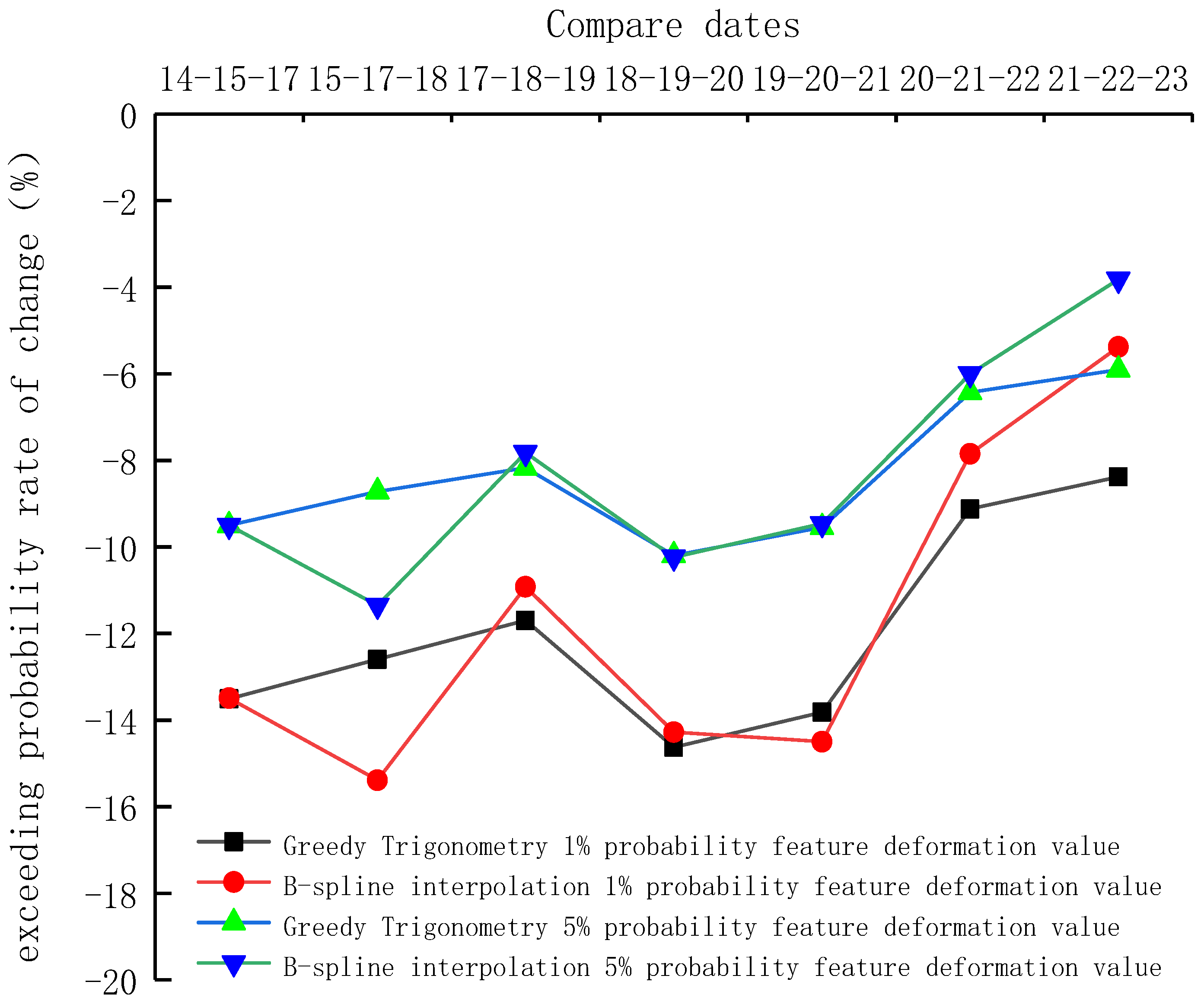
	Positive 5% probability feature deformation value	16.30%	−45.14%	23.63%	−8.25%	−57.67%	−57.07%

shows that the trend of K_n of the 1% probability feature deformation value is approximately in line with that of the 5% probability feature deformation value. The result of the B-spline interpolation method showed significant inconsistency, and the greedy triangulation method’s judgment results were more stable and suited for assessing the initial support deformation in engineering.

Figure 9 and Figure 10 show a symmetrical connection between positive and negative deformations. Further, the 5% probability feature deformation value curve was compatible with the 1% probability feature deformation value curve, whose fluctuation of deformation value was substantially more steady. Similarly, the trends of observations obtained from the greedy triangulation and B-spline interpolation methods were comparable. The B-spline interpolation underwent a mutation for a few days; however, after the mutation, the deformation became consistent with the greedy triangulation method.

7. Discussion

Considering that the 3D laser scanning point cloud is in the scattered form, a surface fitting is required. Compared to the B-spline interpolation method, the results of the greedy triangulation method coincided well with the fitting surface, showing better goodness of fit. Further, when the density of the point cloud was high enough, the curvature of the edges of the triangles in the fitted surface was reduced. When the abrupt change in curvature is minimal, it is possible to assume that the tunnel displacement is in the normal direction of the surface.

Moreover, the normal vector was found to be perpendicular to the first fit. The displacement of the tunnel at this location (which was a vector itself) was the length of the line segment at the point of intersection of the normal vector and two fitted surfaces. A normal matrix can be formed by uniformly arranging normals on a surface. The normal vector matrix accurately expressed the deformation of each position of the tunnel. It is reasonable to assume that the tunnel surface deforms in the normal direction mostly. However, this assumption may not stand correct when the tunnel flatness is seriously insufficient; thus, it is necessary to ensure that the tunnel is flat enough before monitoring.

In this paper, the maximum entropy method was employed to form the probability density function of the normal vector. The authors reflected the deformation trend of the tunnel through the changing trend of the eigenvalues of the normal vector probability density function. This method can not only eliminate the abnormal points caused by the insufficient flatness of the tunnel surface but also fully extract reliable information about the tunnel deformation. The entire deformation of the tunnel may be accurately identified in space. The research also discovered that when the tunnel deformation is small, the normal vector is small, and the probability density function calculation of the maximum entropy method does not converge. If this continues, we may say that the tunnel deformation has stabilized. It was observed in the current study that the 1% probability feature deformation value and the 5% probability feature deformation value could make an accurate judgment. It may be deduced that when the exceedance probability is too small, it is more likely to be disturbed by construction factors. Furthermore, the 5% probability feature deformation value may more accurately depict the deformation of each section of the tunnel.

In future studies, different methods can be used to form the probability density function, and the change in the normal vector matrix can be identified through AI algorithms to judge the deformation trend of the evaluated tunnel.

8. Conclusions

Using the greedy triangulation method to fit the tunnel point cloud, the tunnel fitting surface completely coincided with the fitting surface. The normal vector matrix was created by making the normal of the fitted surface consistent and intersecting with another fitted surface, assuming that the tunnel surface was deformed towards the normal. In this paper, the normal vector matrix was used to characterize the tunnel deformation for the first time, and the probability density function of the normal quantity was formed by the reliability theory of the maximum entropy method. It is proposed to use the probability characteristic deformation value of the normal vector to analyze the trend of tunnel deformation and realize tunnel deformation prediction.

References

- Yang, Y.; Zhang, Y.; Tan, X. Review on Vibration-Based Structural Health Monitoring Techniques and Technical Codes. Symmetry 2021, 13, 1998. [Google Scholar] [CrossRef]
- Qiu, Z. Analysis of tunnel monitoring measurement data based on the optimum weighted combinatorial prediction model. J. Yangtze River Sci. Res. Inst. 2016, 33, 53–56. [Google Scholar]
- Liang, X. Regression analysis and application of monitoring measurement data of new Austrian tunneling method. Build. Technol. 2017, 48, 1188–1190. [Google Scholar]
- Gao, W. Numerical simulation and monitoring analysis of shallowly buried bias tunnel excavation. Constr. Technol. 2011, 40, 48–50. [Google Scholar]
- Yang, Y.; Lu, H.; Tan, X.; Chai, H.K.; Wang, R.; Zhang, Y. Fundamental mode shape estimation and element stiffness evaluation of girder bridges by using passing tractor-trailers. Mech. Syst. Signal Process. 2022, 169, 108746. [Google Scholar] [CrossRef]
- Fekete, S. Integration of 3D laser scanning with discontinuum modeling for stability analysis of tunnel in blocky rockmasses. Int. J. Rock Mech. Min. Sci. 2013, 57, 11–23. [Google Scholar] [CrossRef]
- Vosselman, G.; Maas, H.G. Airborne and Terrestrial Laser Scanning; CRC Press: New York, NY, USA, 2010. [Google Scholar]
- Yang, B.; Liang, F.; Huang, R. Progress, challenges and perspectives of 3d lidar point cloud processing. J. Surv. Mapp. 2017, 46, 1509–1516. [Google Scholar]
- Cai, J.; Zhao, Y.; Li, Y. A 3D laser scanning system design and parameter calibration. J. Beijing Univ. Aeronaut. Astronaut. 2018, 44, 2208–2216. [Google Scholar]
- Wei, Z.; Ding, Z.; Zhou, Z.; Huang, Y. Feasibility Study on Non-contact Measurement Method for Primary Support of Tunnel. Int. J. Geosynth. Ground Eng. 2021, 7, 52. [Google Scholar] [CrossRef]
- Wu, Y.; Zhang, M.; Wang, L. Research on 3D scanning detection technology and application of shield tunnel structure. Mod. Tunn. Technol. 2018, 55, 1304–1312. [Google Scholar]
- Chen, F.; Wang, Y.; Ji, F. Research on 3d laser scanning and 3d contrast technology. Constr. Technol. 2019, 48, 25–29. [Google Scholar]
- Xiang, L.; Ding, Y.; Wei, Z.; Zhang, H.; Li, Z. Research on the Detection Method of Tunnel Surface Flatness Based on Point Cloud Data. Symmetry 2021, 13, 2239. [Google Scholar] [CrossRef]
- Su, J. Studies on Image Interpolation Based on the B-Spline Scheme. Master’s Thesis, Guangdong University of Technology, Guangzhou, China, 2014. [Google Scholar]
- Liu, S.; Han, X.; Jia, C. Grid stitching and fusion of cubic B-spline interpolation. Chin. J. Image Graph. 2018, 23, 1901–1909. [Google Scholar]
- Temlyakov, V. Greedy approximation. Acta Numer. 2008, 17, 235–409. [Google Scholar] [CrossRef]
- Barron, A. Universal approximation bounds for superposition of n sigmoidal functions. IEEE Trans. Inform. Theory 1993, 39, 930–945. [Google Scholar] [CrossRef] [Green Version]
- Chen, C. The Application of Greedy Algorithm in Sparse Learning. Ph.D. Thesis, Hubei University, Wuhan, China, 2016. [Google Scholar]
- Wang, E. Research on 3D Laser Point Cloud Surface Reconstruction Technology. Master’s Thesis, Wuhan University, Wuhan, China, 2019. [Google Scholar]
- Liu, X. Research on 3D Measurement Method of Blade Based on Robot Line Laser Scanning. Master’s Thesis, Harbin Institute of Technology, Harbin, China, 2020. [Google Scholar]
- Liu, B. Surface Fitting Based on Delaunay Triangulation. Master’s Thesis, Tianjin University, Tianjin, China, 2007. [Google Scholar]
- Klaus, V. Drill and blast excavation forecasting using 3D laser scanning. Geomech. Tunn. 2017, 10, 298–316. [Google Scholar]
- Zhao, G. Structural Reliability Theory; Construction Industry Press: Beijing, China, 2000. [Google Scholar]
- Meng, Q. Information Theory; Xi’an Jiaotong University Press: Xi’an, China, 1989. [Google Scholar]
- Siddle, J. Probability Engineering Design: Principle and Application; Marcel Dekker Inc.: New York, NY, USA, 1983. [Google Scholar]
- Zhang, X.; Ma, L. Entropy Meteorology; Meteorological Press: Beijing, China, 1992. [Google Scholar]
- Silvin, G. Information Theory with Application; McGraw-Hill: New York, NY, USA, 1977. [Google Scholar]
- Yang, L. Reliability index calculation of concrete arch dam by a combined stochastic FEM and maximum entropy method. J. Water Conserv. Water Transp. Eng. 2003, 2, 24–28. [Google Scholar]
- Yang, Y.; Li, J.; Zhou, C.; Law, S.; Lv, L. Damage detection of structures with parametric uncertainties based on fusion of statistical moments. J. Sound Vib. 2019, 442, 200–219. [Google Scholar] [CrossRef]
- Yang, Y.; Li, C.; Ling, Y.; Tan, X.; Luo, K. Research on new damage detection method of frame structures based on generalized pattern search algorithm. J. Instrum. 2021, 42, 123–131. [Google Scholar]
- Wei, Z. Prediction of failure mode of single-layer spherical reticulated shell under earth-quake based on maximum entropy method. Vib. Shock 2008, 27, 64–69. [Google Scholar]
- Wei, Z.; Ye, J.; Shen, S. Engineering application of the maximum entropy reliability theory. Vib. Shock 2007, 26, 4. [Google Scholar]
- Goodman, R.; Shi, G. Block Theory and Its Application to Rock Engineering; Prentice Hall: Englewood Cliffs, NJ, USA, 1985. [Google Scholar]
- Liu, J. Theory and Application of Key Blocks; Water Resources and Hydropower Press: Beijing, China, 1988. [Google Scholar]
- Liu, F.; Zhu, Z.; Sun, S. Block theory and its application in stability analysis of cavern surrounding rock. Chin. J. Undergr. Space Eng. 2006, 2, 1408–1412. [Google Scholar]
- Wei, Z.; Yao, T.; Shi, C. Research on the Construction of 3D Laser Scanning Tunnel Point Cloud Based on B-spline Interpolation. In Proceedings of the GeoChina 2021 International Conference, Nanchang, China, 18–19 September 2021; Volume 8, pp. 111–118. [Google Scholar]
- Wei, Z.; Yu, M.; Zhou, Z. Analysis of Tunnel 3D Laser Scanning Detection and Monitoring Accuracy. Mod. Tunn. Technol. 2020, 57, 5. [Google Scholar]
- Yang, Y.; Ling, Y.; Tan, X.; Wang, S.; Wang, R. Damage identification of frame structure based on approximate Metropolis–Hastings algorithm and probability density evolution method. Int. J. Struct. Stabil. Dyn. 2022, 22, 2240014. [Google Scholar] [CrossRef]
Figure 1.
The layout of measuring points of traditional monitoring and measurement method.
Figure 2.
Flowchart of tunnel monitoring and measurement algorithm.
Figure 3.
Schematic diagram of tunnel fitting surface.
Figure 4.
Schematic diagram of the probability density function of the initial support deformation of the tunnel.
Figure 5.
Schematic diagram of the deformation direction of the surface fitted by the B-spline interpolation method on the 14th–15th days (Note: the deformation direction of the golden part is outward, and the deformation direction of the red part is inward).
Figure 6.
Schematic diagram of the deformation direction of the surface fitted by the B-spline interpolation method on the 15th–17th day (Note: the deformation direction of the golden part is outward, and the deformation direction of the red part is inward).
Figure 7.
Comparison of positive deformation trends.
Figure 8.
Comparison of negative deformation trends.
Figure 9.
Comparison of positive feature deformation between greedy triangulation and B-spline interpolation.
Figure 10.
Comparison of negative feature deformation between greedy triangulation and B-spline interpolation.