Temporal-Spatial Nonlinear Filtering for Infrared Focal Plane Array Stripe Nonuniformity Correction


1
School of Physics and Optoelectronic Engineering, Xidian University, Xi’an 710071, China
2
Department of Basic, Air Force Engineering University, Xi’an 710051, China
*
Author to whom correspondence should be addressed.
Symmetry 2019, 11(5), 673; https://doi.org/10.3390/sym11050673
Submission received: 29 April 2019
/
Revised: 11 May 2019
/
Accepted: 13 May 2019
/
Published: 15 May 2019
Abstract
:In this work, we introduce a temporal-spatial approach for infrared focal plane array (IRFPA) stripe nonuniformity correction in infrared images that generates visually appealing results. We posit that the nonuniformity appears as a striped structure in the spatial domain and that the pixel values change slowly in the temporal domain. Based on this, we formulate our correction method in two steps. In the first step, weighted guided image filtering with our adaptive weight is utilized to predict the stripe nonuniformity using a single frame. In the second step, the temporal profile of each pixel can be formed using a few frames of successive nonuniformity images. Further, we present a temporal nonlinear diffusion equation to remove scene residuals from the temporal profile of nonuniformity images in order to estimate a more accurate value of the stripe nonuniformity. The results of extensive experiments demonstrate that the proposed nonuniformity correction algorithm substantially outperforms many state-of-the-art approaches, including both traditional and deep convolution-neural-network-based methods, on four popular infrared videos. In addition, the proposed method only requires a fraction (less than ten) of the video frames.
1. Introduction
In many applications, such as drone-based infrared video surveillance and early warning systems, one must process images and videos that contain undesirable artifacts such as stripe nonuniformity, which is caused by the unidentical response rates to the same infrared radiation intensity among infrared detector units [1]. Furthermore, the performance of many infrared search and tracking systems often degrades when they are presented with images that contain such artifacts. Hence, it is important to develop algorithms that can automatically remove these artifacts. To address the problem of stripe nonuniformity correction (NUC), various methods [2,3,4,5,6,7,8,9] have been proposed in the literature.
The widely used NUC methods in practical application are calibration-based methods [2,3]. State-of-the-art calibration-based NUC methods, such as one-point, two-point, and multipoint correction, often suffer from response characteristic drift of the infrared detector after working only one hour or less, as shown in Figure 1. Overcoming this problem requires calibrating the detector to correct the parameter drift periodically. However, this solution scheme will heavily affect the performance in infrared video surveillance, early warning, and other applications. Hence, more adaptive and efficient methods that can deal with nonuniformity are needed.
One solution to this problem is utilizing a scene-based NUC framework [4,5,6,7]. Scene-based NUC methods estimate the calibration parameters from the scene. It relies only on real scene information that is acquired by the infrared imaging system for obtaining the drift correction parameters. This has been realized by many scholars. They leveraged many sequential frames or a single frame in a video to remove the stripe nonuniformity from infrared images [8,9]. However, a drawback of the sequential-frame-based algorithms is that these algorithms are required for convergence. Another drawback of these algorithms is that the corrected image contains ghost artifacts and image degradation. In contrast, the single-image-based NUC algorithms use only structural features of nonuniformity in the spatial domain and do not effectively consider its low-frequency characteristics in the temporal domain. Thus it is difficult to improve the correction effect and suffers from an issue of complex implementation, especially in the presence of strong noise.
To address these problems, we propose a novel NUC method which uses the temporal and spatial information of sequential frames in a video to correct the stripe nonuniformity adaptively. The proposed method consists of two main stages: single-frame-based spatial domain filtering and multi-frame-based temporal domain filtering. The stripe NUC algorithm considers the gradient of the image in calculating the global weight map for estimating the stripe nonuniformity preliminarily. Further, we construct a nonlinear diffusion equation to process the temporal profile of the nonuniformity image sequence, which is used to estimate the more accurate nonuniformity values with the gray values of the same pixels before and after. Once the nonuniformity has been estimated, we fuse the estimated nonuniformity information to input a video frame to obtain the final nonuniformity correction output. Our algorithm differs from existing scene-based NUC methods in the following three aspects:
- The proposed NUC algorithm accurately determines the nonuniformity information and efficiently removes the corresponding nonuniformity under the guidance of the estimated nonuniformity label. Due to the nonlinear filtering used in the temporal domain, our method requires fewer sequential frames in a video to realize more accurate correction results. In addition, it does not have the problem of slow convergence and ghosting artifacts.
- Based on the observation that a weighted guided image filter can be used as a satisfactory nonuniformity estimate in the spatial domain, a novel global weight map sensitive to stripe noise is introduced into the guided image filter to improve its efficiency in suppressing stripe noise and preserving edge information.
- Compared with the single-frame-based NUC methods, our proposed method makes full use of the temporal characteristic of the nonuniformity to substantially improve the nonuniformity estimation accuracy. Consequently, the degradation of the corrected image is greatly reduced.
The remainder of the paper is organized as follows: Section 1 discusses the related work in the field of nonuniformity correction. Section 2 describes the weighted guided image filter and proposed a global weight map, which is a key component of our method. Section 3 discusses the proposed method in detail. Section 4 presents our quantitative and qualitative evaluations. Finally, Section 5 presents the conclusions of our paper.
2. Related Works
There is a long history of work in infrared focal plane array (IRFPA) stripe nonuniformity correction. Here, we briefly review several recent related works on scene-based NUC and NUC formation.
2.1. Scene-Based Nonuniformity Correction
Scene-based NUC methods have good adaptivity in parameter drift correction. Generally, scene-based NUC algorithms can be divided into sequence-image-based correction and single-image-based correction. Sequence-image-based NUC methods are seeking to make a reasonable estimate for model parameters through the statistical information of image sequences and reasonable assumptions. Temporal high-pass filter (THPF) [4], neural networks (NN) [5], and constant statistics (CS) [10] are traditional NUC methods, which are categorized as statistical-based NUC methods. Serious ghost artifacts and image degradation will occur in the correction process of these methods. To improve the property of the THPF-based NUC methods, Qian et al. [11] and Zuo et al. [12] combined low-pass filter and bilateral filter with THPF to correct the nonuniformity in each video frame. On the basis of literature [12], Li et al. [13] made use of high brightness region detection to adjusting temporal filtering coefficients to improve correction performance. Similarly, many scholars have improved the NN and CS correction algorithm. Zhang et al. [14] and Lai et al. [15] ameliorated NN NUC method via partial differential equations and total-variation-penalized neural network regression. Hardie et al. [16] applied an adaptive threshold to update statistical parameter estimate in CS-NUC. Zhou et al. [17] proposed a multi-frame statistics based nonuniformity correction method for airborne infrared imaging systems. Afterward, the registration-based methods were proposed, and they assume that the response of each detector to the same scene is identical and the difference is on account of the nonuniformity. Hayat first proposed the registration-based NUC method [18] and some scholars also proposed several methods by extending this kind of methods [19,20]. These methods need fewer frames of an image than the statistical-based methods and have almost no ghosting artifacts. The key to this kind of algorithm is the accuracy of registration results. In recent years, methods for single-frame infrared image nonuniformity correction have also been developed. These methods include a body of work on stripe nonuniformity correction. Tendero et al. [21] used midway equalization to predict the nonuniformity. More recently, Kuang et al. [22] utilized deep convolutional neural networks to directly predict the correction result. He et al. [23] used deep residual networks to end-to-end estimate the nonuniformity. Zeng et al. [24] proposed a two-stage filtering NUC method which was suitable for stripe FPN correction.
More closely related to our work are the approaches that combine spatial filter and temporal filter, such as those presented in References [11,12,13]. In these papers, the raw image was first separated into low-frequency components and high-frequency components by low pass filter or edge-preserving filter in the spatial domain and then the high-frequency components were processed by high-pass filter in temporal to correct nonuniformity. The key point is the image separation into two parts. If there are too many image edge detail residuals in the high-frequency components that decomposition from raw images by filtering, the image degradation will be more serious in corrected images. In contrast, we address the task of stripe nonuniformity correction by applying WGIF with our adaptive weight to separate the raw image in the spatial domain, which has a better performance of non-uniformity and scene separation effect, and in the temporal domain a non-linear diffusion equation is proposed to deal with the nonuniformity sequence so that the nonuniformity correction needs only a few frame images.
2.2. Nonuniformity Correction Formation
In an infrared focal plane array, the response of each detector unit is linear in a range and the response characteristic of each infrared detector is constant over a short period of time. Mathematically, a response characteristic function, which is denoted as y, can be modeled as a linear combination of the incident irradiance x with a gain coefficient and a bias coefficient as follows:
Here, for an infrared focal plane array, the response characteristic function, namely y, is a standard reference function. The objective is to recover x from the observed image. The two coefficients will change the response characteristic of a detector unit such that the image acquired by this detector will contain nonuniformity. Especially in a linear array detector and uncooled infrared imaging system, the nonuniformity looks like the stripe noise. Therefore, we should constantly adjust these two parameters to the initial values during the operation. However, the bias coefficient will vary widely, whereas the gain coefficient changes only slightly. Hence, the influence of the gain change can be neglected under normal conditions [25]. Based on this observation, the model can be simplified as follows:
According to the model (Equation (2)), our objective is to obtain the initial value of x from a given y, where can be viewed as the stripe nonuniformity. To accomplish this, we transform this problem into image pixel estimation to bias .
3. Weighted Guided Image Filtering and Global Weight Map
The weighted guided filter (WGIF) [26] was proposed by affiliating an edge-aware global weight map with a guided image filter (GIF) [27], and has been widely used in several vision tasks, including image detail enhancement [28], image haze removal [28] and multiexposure image fusion [29]. In virtue of the global weight map, WGIF is provided with excellent properties of both global and local smoothing filters. The global smoothing filters show a good performance in edge preserving, while the local smoothing filters have low complexity. In its framework, the output image is a linear transform of the guidance image I in a window that is centered at pixel k:
where and are constant coefficients in window , which can be estimated by minimizing the following cost function:
the optimal values of a and b are calculated via Formulae (5) and (6):
where X is the original image, represents the number of pixels in window , and are the mean values of I and X in , is the variance of I in , represents the regulation parameter, and W is the global weight map that measures the likelihood of being on the edge of each pixel in the guidance image. The final output image, which is processed via WGIF, is expressed as follows:
where and are the mean values of and , respectively, in window .
In WGIF, the filtering performance depends heavily on the global weight map, namely, W. In literature [26], the variance of the guided image in a local window is used to calculate the weight W and realize satisfactory edge preservation performance. Moreover, the Sobel gradient operator and the Robert gradient operator can be used to calculate the weight to improve the filtering performance of GIF. Subsequently, a gradient domain GIF (GGIF) [30] was proposed to improve the property of edge-preserving of WGIF. In this paper, we design a new kernel function for calculating the weight, which is more specific in suppressing stripe nonuniformity while preserving edges.
3.1. Analysis of the Global Weight Map
In WGIF, pixels that have smaller weights will be smoothed to a higher degree, while pixels that have larger weights will be smoothed to a lower degree. For an IR image that contains stripe nonuniformity, larger weights should be assigned to the edge details and the stable background to protect these areas from being smoothed, while smaller weights should be assigned to the stripe nonuniformity so that these areas will be smoothed to remove the stripe noise. The gradient of the pixels can be used to determine in which area the pixels are located: The edge detail area, the stripe noise area or the stable background area. That is, the pixels that are on the edges must correspond to large gradient values, whereas on a stable part of the image, the change of the gray value is smaller and the corresponding gradient is also smaller. For the pixels that are overlaid stripe nonuniformity, the energy of the horizontal gradient is increased, while the gradient in the vertical direction is very small [31]. The gradients of the four directions of each pixel in the image can be expressed as follows:
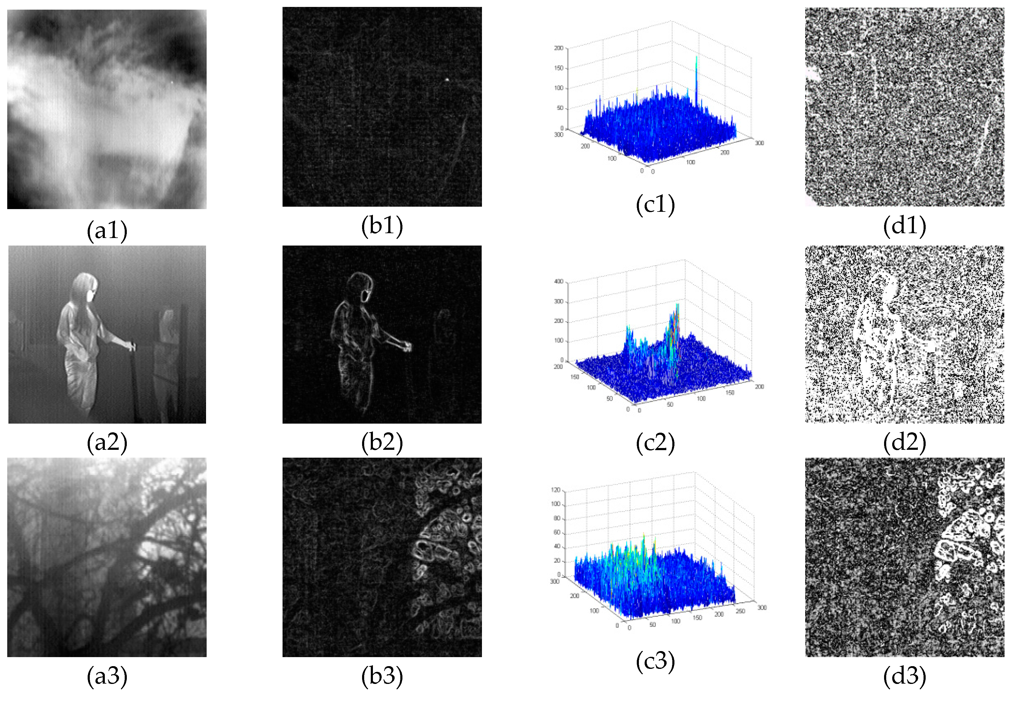
To clearly show the four direction gradients of each pixel , Figure 2b1–b3,c1–c3 give the gradient images for three different infrared images and their corresponding 3D gradient maps. It can be seen that the gradient values are larger at the edges than other regions from Figure 2b1–b3. Especially for the targets regions, the gradient values are the highest in the gradient map. Meanwhile, the gradient values of the stable background are very small. By contrast, the gradient values of the regions containing nonuniformity are higher than that of stable background regions but lower than that of the edge regions, as shown in Figure 2b1–b3,c1–c3.
3.2. Kernel Function
According to the analysis above, we proposed the following inverted Gaussian function as the kernel function to process the gradient image and obtain the adaptive global weight map W for smoothing strip nonuniformity. The kernel function is defined as follows:
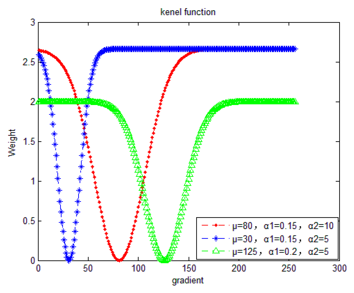
where and are parameters that adjust the maximum value of the weight and the width of valley-shaped curve, respectively, is the mean value of the gradient image, which set the position of the minimum of the curve, is a function that measure the distance from to the median gray level value , which regulate the in Formula (9). is the regularization factor. Figure 3 presents the kernel function with different parameters. The efficiency of can be seen clearly from blue and green curves in Figure 3. The further is from , the larger the value of , so that the smaller is, the narrower the width of the valley-shaped curve is. In this way, when the average gray value of gradient image is small, the area of smaller the gradient image will be protected from over-smoothed. So that the suppression ranges are adjusted adaptively according to . Thus we can alter the smoothed area and smooth degree by setting the parameters. Figure 2d1–d3 are the gradient images that have been processed by the kernel function, namely, the global weight maps. In the weight maps, bright areas represent greater weight.
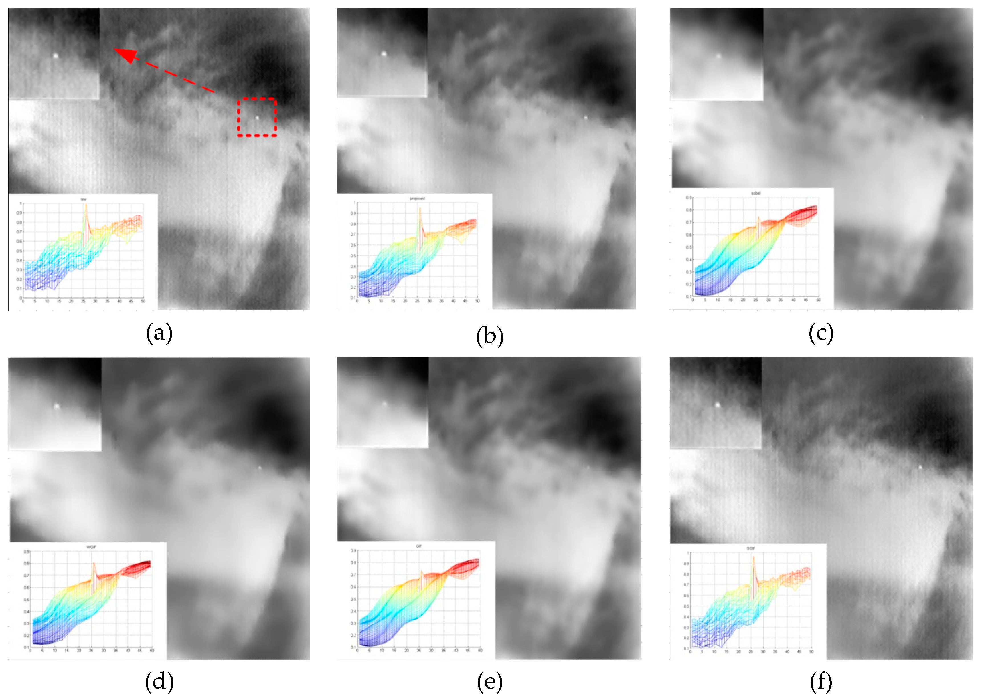
To clearly show the performance of WGIF with different global weight maps, GGIF, and GIF, we select an infrared video with a small target in sky background. To show the results clearly, the region of 48 × 48 around the small target is zoomed and displayed in the upper left corner of the image. At the same time, this region is also displayed by 3D image and displayed in the bottom left corner of the image. Figure 4 gives the results obtained by these filters. From Figure 4, GIF, WGIF with Sobel operator and the weight map proposed in the literature [26] perform excellently in stripe noise removing, but the scene details are somewhat blurred, especially, the intensity of the target is weakened. We can see this phenomenon clearly from the 3D images (the sharp pulse in the 3D image is the intensity of the small target). What is more, the image filtered by GGIF preserves abundant scene details. However, there are serious stripe nonuniformity residuals in the filtered image, as shown in Figure 4f. In contrast, WGIF with our proposed weight map has a good ability to remove non-uniformity, while preserving details of the image, especially the intensity of small targets. In conclusion, the filtered result of WGIF with our weight map is more ideal in stripe nonuniformity removing and scene details preserving.
4. Proposed Method
The stripe nonuniformity is characterized by vertical stripe noise in the spatial domain and slow-changing values in the temporal domain. Based on this, our goal is to make full use of the spatial and temporal characteristics of stripe nonuniformity to propose a stripe nonuniformity correction method. Figure 5 illustrates the overall architecture of our proposed method. Following the strategy, our method consists of two main parts: spatial domain nonuniformity coarse estimation and temporal domain nonuniformity fine estimation. Given an infrared video that contains nonuniformity, we attempt to produce a coarse nonuniformity via weighted guided image filtering with our designed global weight map in spatial domain module. The coarse nonuniformity contains not only nonuniformity but scene residuals as well. The temporal module will use a nonlinear diffusion equation to process temporal profiles of each pixel for separating the scene residuals from nonuniformity images. Once the nonuniformity has been accurately identified, we can easily remove it from the source infrared video by subtracting the corresponding frame in the input video.
4.1. Spatial-Domain Nonuniformity Estimation via Weighted Guided Image Filtering
In the first step, we aim to estimate the stripe nonuniformity using a single frame image. An observed image X is filtered by WGIF with our proposed global weight map to produce an ideal image without stripe nonuniformity, namely, B. Simultaneously, we chose X as the guidance image. Then, the stripe nonuniformity d can be easily obtained by subtracting this ideal image from the source input image as follows:
Figure 6 shows the simulated results of the Formula 13. The observed images are in Figure 6a1,a2, namely X (b1,b2) represent the ideal image B (c1,c2) are the stripe nonuniformity images. According to Figure 6c1,c2, the scene residuals still exist in the stripe nonuniformity images. Hence, the corrected image will suffer from quality degradation and the loss of important information, such as small targets and details. To address this problem, we propose a nonlinear diffusion equation to process the pixel temporal profile for estimating the more accurate value of the nonuniformity to remove the scene residuals from the nonuniformity images.
4.2. Temporal-Domain Nonuiformity Correction Via a Nonlinear Diffusion Equation
In the second step, we attempt to remove the scene residuals from the nonuniformity images taking advantage of the different characteristics of nonuniformity and scene residuals in temporal domain, so as to estimate more accurate nonuniformity values. temporal profile is a curve describing the change of a pixel in a continuous frame image. Figure 7a,b shows the formation of the temporal profile and two temporal profiles in the nonuniformity image sequence, respectively. According to Figure 7b, the pixel values of the nonuniformity change slowly in sequent images (see the blue curve), while the values of the moving scene residuals exhibit drastic fluctuations (see the red curve). In order to eliminate the mutation points in stationary curves, i.e., scene residuals in nonuniformity images, we construct a nonlinear diffusion equation to process the temporal profiles for obtaining more accurate nonuniformity values.
Suppose is the temporal profile of a pixel p in a nonuniformity sequence at time t. The diffusion function can be expressed as follows:
where n refers to the n-th frame in a video sequence, denotes the gradient at point n of the curve, and function is adopted as a nonlinear diffusion coefficient. We expect higher diffusion degrees at points with larger gradient values. Hence, function is defined as follows:
where r denotes the regularization parameter.
Since the temporal profile consists of discrete one-dimensional data, Equation (14) can also be expressed as Equation (16) when the diffusion equation is used to smooth the curve.
where , , m is the number of iterations, and denotes the adjustment parameter.
To illustrate the efficiency of the proposed nonlinear diffusion equation filtering, Figure 8 presents the output processed by the diffusion equation. In Figure 8, the red curves correspond to the temporal profiles of a pixel over 20 frames in the stripe nonuniformity image sequence, and the blue curves are the results processed by proposed diffusion equation, namely, estimated more accurate stripe nonuniformity values. The red curve in Figure 8a shows small fluctuations that mainly correspond to stripe noise, while the red curve in Figure 8b shows violent fluctuations that correspond to the movement scene edge details residuals. From the blue curve, it can be seen that the proposed temporal method can eliminate the values with a large difference to adjacent values, no matter the gradual curve or the curve with a sharp change, so as to get more accurate non-uniformity value.
Finally, the nonuniformity can be obtained via Equation (17) and the n-th frame of the corrected image, which is denoted as can be calculated as follows:
where .
5. Experiment and Analysis
In this section, the performance of the proposed method is tested. Experiments on four representative real IR image sequences that were obtained by an uncooled infrared camera (8–12 μm) were conducted. For four IR image sequences, we carried out two simulation experiments. The quantitative evaluation and qualitative comparison with four NUC methods are presented to evaluate our method more objectively.
Four sequences are shown in Figure 9. Sequence 1 contains with a stable background and a walking girl. The images are of size 180 × 200. We evaluate the correction performance of NUC methods for a stable background with a moving object using this sequence. Sequence 2 has a scene that contains a small target that is moving with high velocity against a complex cloud background (The position of the small target is framed by a red dotted line). The images are of size 256 × 256. This sequence can be used to evaluate the preservation of small targets in IR images that are processed via these NUC methods. Sequence 3 was obtained by a moving camera. Hence, the entire scene has the same motion. The images are of size 128 × 128. The scene in Sequence 3 has abundant details. Therefore, we can evaluate the performance of NUC methods on this complex moving scene. We select Sequence 4, in which the images are of size 150 × 200, as the testing sequence for its strong horizontal and vertical edges. The preservation performance on strong edges is evaluated. In addition, we compared our method with four representative methods: TVRNN-NUC [15], BF-THPF NUC [12], MIRE NUC [21] and CNN NUC [23].
5.1. Objective NUC Quality Metrics
To quantitatively evaluate the NUC performance, two metrics are considered: The residual nonuniformity, which is denoted as U, and the roughness parameter, which is denoted as ρ [31].
The residual nonuniformity, namely, U, is defined as follows:
where and are the intensity of pixel (i,j) and the mean value of the corresponding frame, respectively. M and N denote the numbers of rows and columns of the infrared focal plane array detector units, and l and h are the numbers of dead pixels and overheated pixels, respectively, in IRFPA. A smaller residual nonuniformity value corresponds to higher performance of the NUC method.
The roughness parameter is defined as follows:
where X is the input image, h1 = [1, −1] is a horizontal mask, h2 = [1, −1]T is a vertical mask, and denotes the L1-norm. Similar to nonuniformity U, a smaller value of is expected in the corrected image.
5.2. Implementation Details
We designed a spatial-temporal nonuniformity correction algorithm and compare it with other methods. The parameter settings of the proposed and compared methods are shown in Table 1.
5.3. Experiment Results and Discussion
5.3.1. Experiment 1
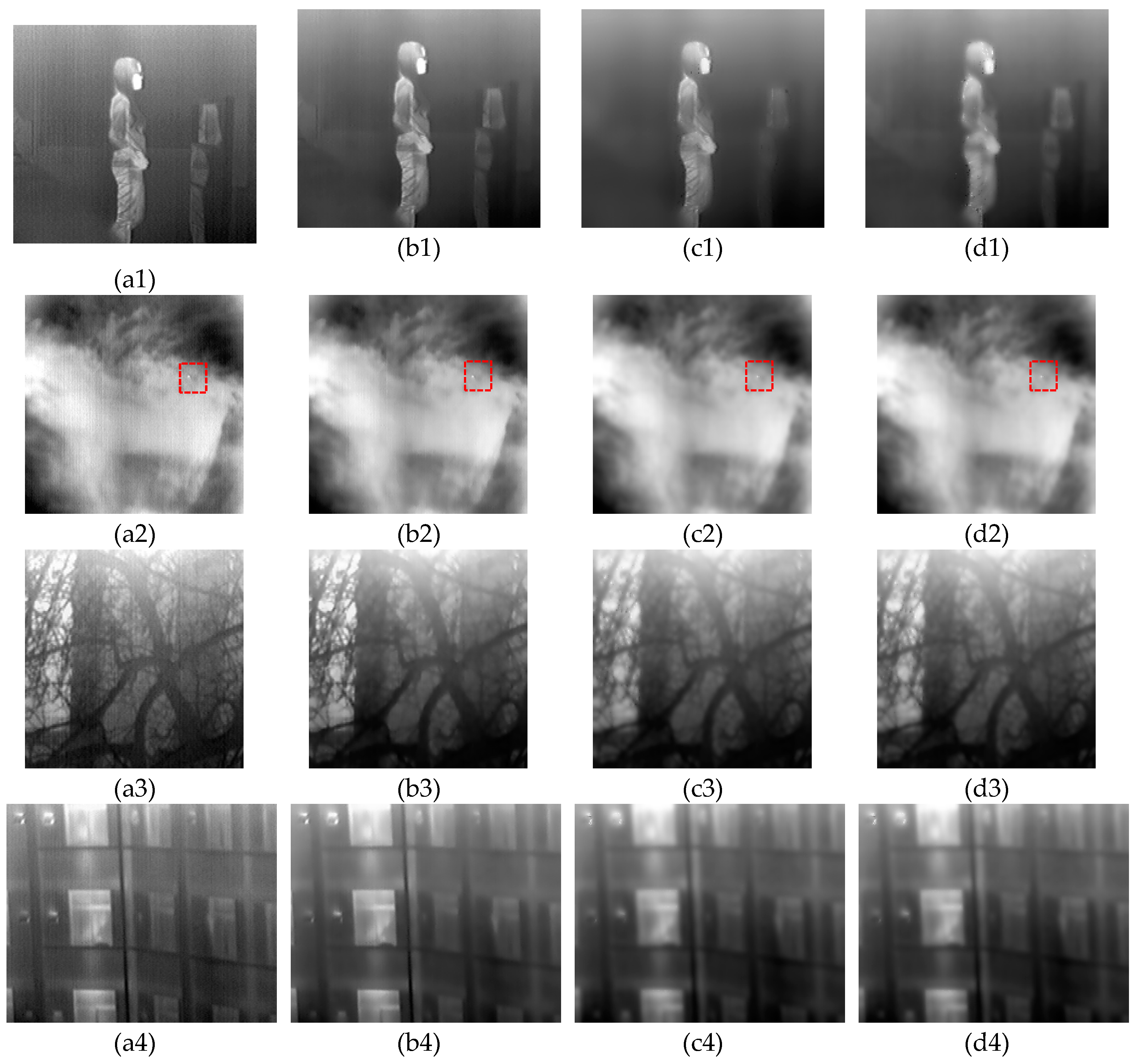
In experiment 1, our aim was to test the effect of different weight maps on the correction results. Four sequences of images were processed by our proposed temporal-spatial domain NUC framework. In spatial domain processing, different weight maps were selected with WGIF. The weight maps were obtained by our proposed method in Section 2.2, literature [26], and the Sobel operator, respectively. The simulation results are presented in Figure 10. Figure 10a1–a4 are four raw images, Figure 10b1–b4 are the corrected images that were processed with the proposed weight map. In Figure 10b1, the stripe nonuniformity is suppressed and the edge details are preserved well, which can be clearly seen from the texture of the girl’s trousers. Similarly, the small moving target is well preserved in Figure 10b2. Figure 10c1–c4,d1–d4 are the NUC results that were processed by the weighted maps proposed in the literature [26] and the Sobel operator, respectively. By comparison, we can see that the correction of stripe nonuniformity has got some effects. However, the images were severely degraded during correction, especially on the edge of the walking girl and the windows. In Figure 10c4,d4, it is clear that the small target and the cloud background are blurred. From this experiment, we can confirm that the weight map proposed in this paper has a positive impact on the correction results and plays an important role in this algorithm. This experiment results are due to the reason that our weight is more sensitive to stripe noise, so it can better improve the ability of WGIF in stripe noise suppressing while preserving background edges.
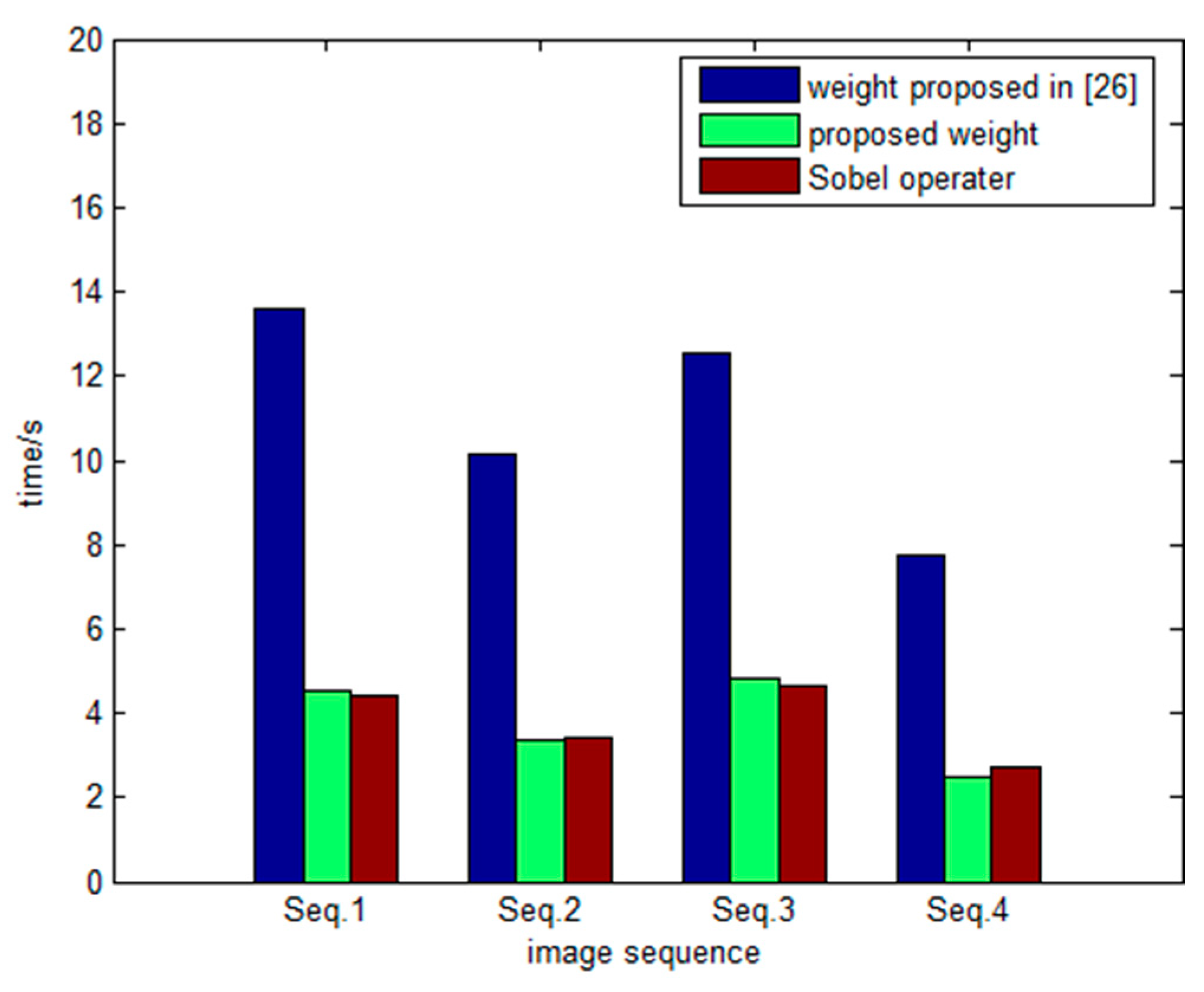
In experiment 1, we also tested the time consuming of our NUC method with different weighted maps. All the tested methods were implemented in Matlab R2014a on a common PC with an Intel Core i5 CPU (3.40 GHz) and 16 GB RAM. In this part, 10 frames of images were used to complete the test. We chose the bar chart to show the computing time for displaying intuitively. From Figure 11, it can be seen that the proposed method and Sobel operator completed the task in less time. In contrast, the weighted map proposed in the literature [26] is more time-consuming.
5.3.2. Experiment 2
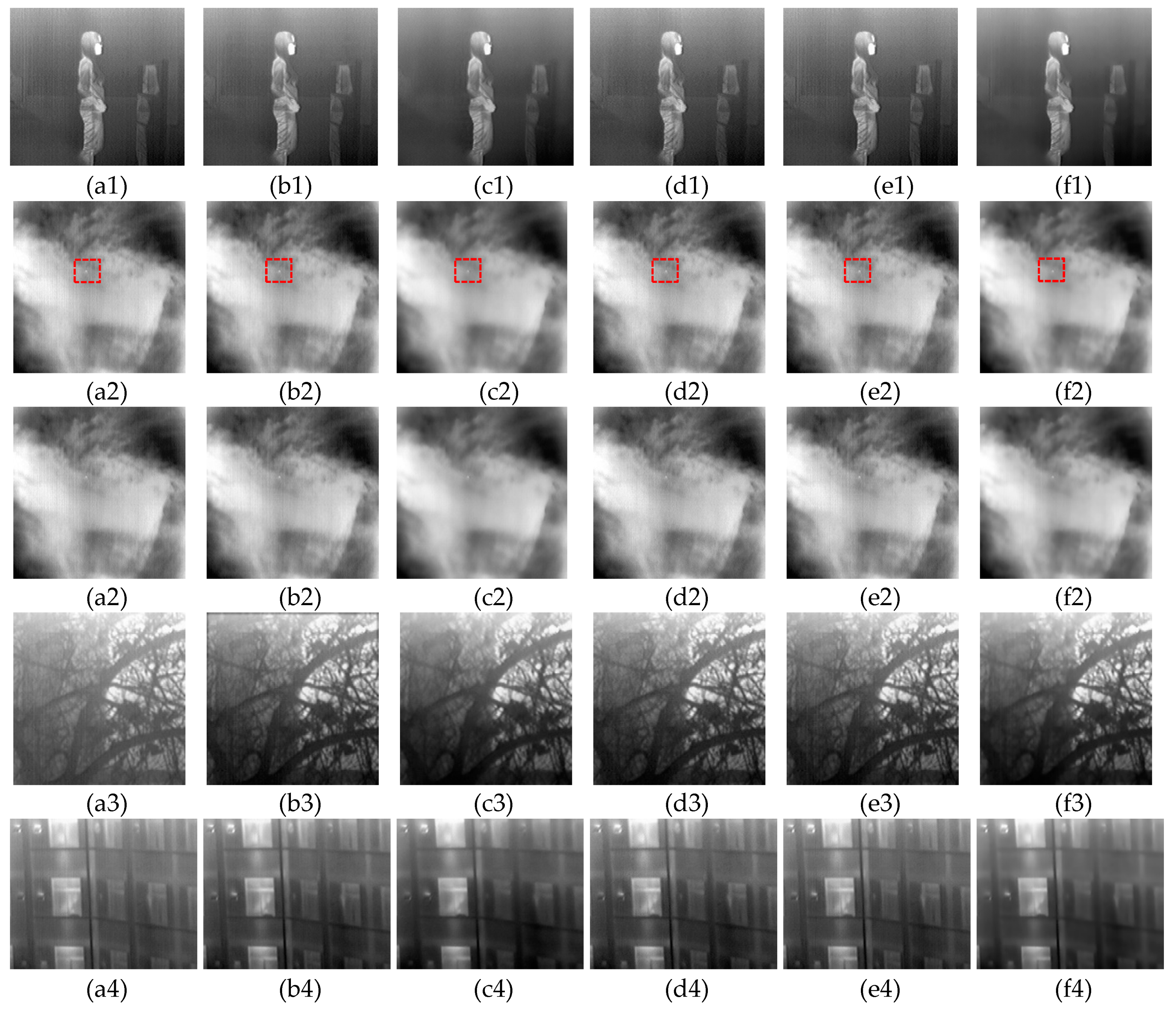
In experiment 2, four representative NUC algorithms were selected to compare with our method in terms of performance. Figure 12 shows the results of TVRNN-NUC [15], BF-THPF NUC [12], MIRE NUC [21] and CNN NUC [23].
The corrected results that were obtained via the TVRNN-NUC method exhibit a correction effect. The advantage of this method is that the image details are preserved well in the process of correction. However, there remains stripe noise in the corrected image, and as the number of corrected frames increases, ghosting artifacts will appear. In addition, the correction results that were obtained via the MIRE and CNN NUC methods are not excellent, they still contain significant nonuniformity artifacts. According to Figure 12d1–d4,f1–f4, the nonuniformity exists in both the complex and the stable scenes of the corrected images. According to Figure 12c1–c4,f1–f4, the BF-THPF NUC method and our method outperform the other methods due to their superior correction performance in visual effects. The BF-THPF NUC method and our method can efficiently remove the nonuniformity in IR image sequences. However, in terms of image detail preservation, the BF-THPF method results in an over-smoothed phenomenon for various detail edges in the image. The reason for this phenomenon is that although bilateral filtering has some adaptive characteristics for image decomposition, it is difficult to adaptively optimize and adjust the geometric features of the image. Therefore, the images will inevitably lead to image blurring and even loss of details. In contrast, our global weights map makes the WGIF perform better in suppressing stripe nonuniformity and preserving edge details in the spatial domain. Therefore, our algorithm can effectively remove the stripe nonuniformity while preserving image edge details.
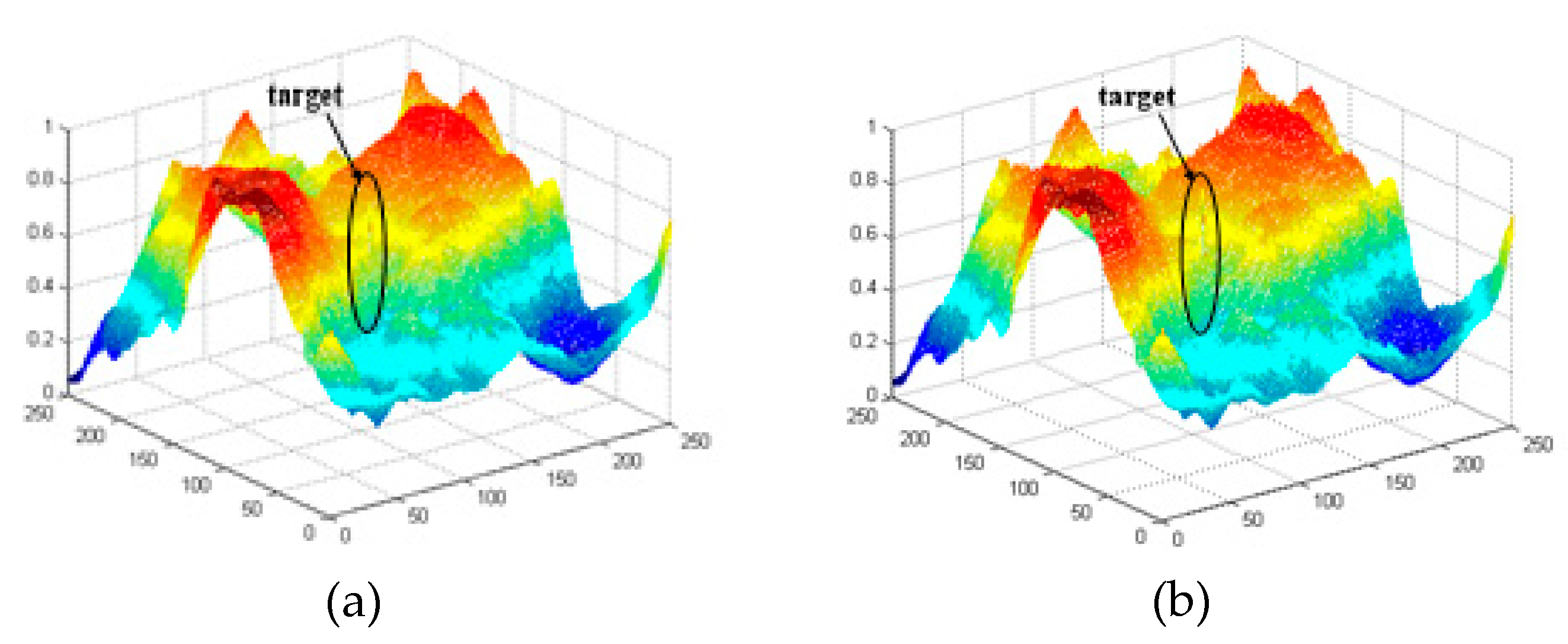
Furthermore, in order to see more clearly the difference between our method and BF-THPF NUC method in scene detail preservation, Figure 13 shows 3D views of the images in Figure 12c2,f2, which were corrected via BF-THPF and the proposed NUC method. The proposed method outperforms BF-THPF NUC in terms of detail preservation (see the moving small target). It can be clearly seen from the 3D image that in the corrected image by our method, the intensity of moving dim and small targets is greater, and it is easier to distinguish from the surrounding scenes.
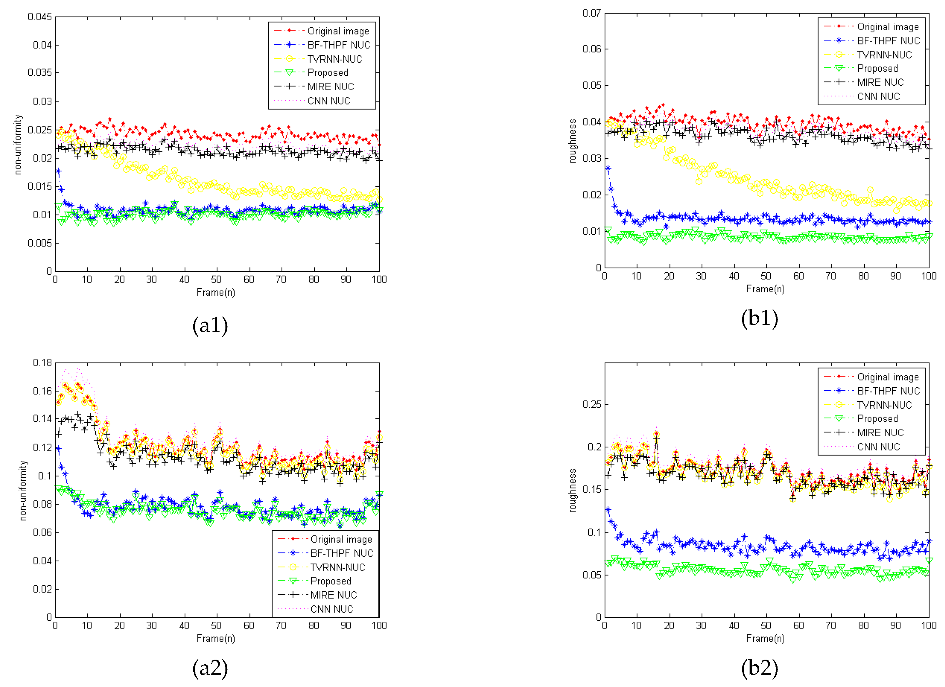
In addition, an objective performance evaluation is also reported in this paper. Two objective metrics, namely, U and are used to quantitatively compare various NUC methods in terms of correction performance. Table 2 lists the values on various tested IR image sequences, in which the bold values indicate the best performance. According to the figures, our method yields smaller values of U and . For example, in Sequence 1, the values of U and are 38.9% and 71.6% lower, respectively, compared to the original image.
To evaluate the robustness of the proposed method, we selected 100 frames of Sequence 1 and Sequence 2 for experiments. From these two objective metrics curves in Figure 14, our method and BF-THPF NUC method have a more excellent performance than the other three methods in 100 frames. By comparing the curves of the two methods, it is obvious that our method has a good correction effect from the first frame, while the bilateral filtering method needs a convergence process to achieve a good correction effect. Combining with the visual effect of the corrected results in Figure 12, the corrected results of our method not only guarantee the lower objective index but also preserve the edge details in the image, which also confirms the superiority of our method. Overall, it is concluded that the proposed method realizes better correction performance than the previous methods according to both visual comparison and objective assessment.
6. Conclusions
We have proposed a temporal-spatial nonlinear filtering-based stripe nonuniformity correction method. The method utilizes our newly designed weighted guided image filter to produce a coarse nonuniformity that contains all the nonuniformity, in addition to scene information. Moreover, our temporal-spatial module uses a diffusion equation for removing the scene information. Once the nonuniformity has been accurately identified, we can easily remove it from the source infrared video by subtracting each corresponding frame from the input video. With this framework, we realized substantial performance gains over four representative NUC methods on three truthful infrared image sequences. Moreover, we demonstrated that the proposed method performs well on only a few frame images.
Author Contributions
Formal analysis, L.J. and Y.X.; funding acquisition, Q.H.; methodology, L.J.; software, L.J. and Z.Q.; supervision, Q.H. and Y.T.; writing—original draft, L.J.; writing—review and editing, Q.H., Y.X. and Z.Q.
Funding
The work was supported by National Natural Science Foundation of China (No. 61401343), the Fund for Foreign Scholars in University Research and Teaching Programs (the 111 Project) (No. B17035), Natural Science Basic Research Plan in Shaanxi Province of China (No. 2017JM6079) and Research Fund Department of Basic Sciences at Air Force Engineering University (JK201910).
Conflicts of Interest
The authors declare no conflict of interest.
References
- Scribner, D.A.; Kruer, M.R.; Killiany, J.M. Infrared focal plane array technology. Proc. IEEE 1991, 79, 66–85. [Google Scholar] [CrossRef]
- Friedenberg, A.; Goldblatt, I. Nonuniformity two-point linear correction errors in infrared focal plane arrays. Opt. Eng. 1998, 37, 1251–1253. [Google Scholar] [CrossRef]
- Sungho, K. Two-point correction and minimum filter-based nonuniformity correction for scan-based aerial infrared cameras. Opt. Eng. 2012, 51, 106401. [Google Scholar]
- Scribner, D.A. Nonuniformity correction for staring IR focal plane arrays using scene-based techniques. In Proceedings of the International Society for Optics and Photonics (SPIE), Washington, DC, USA, 1 September 1990; pp. 225–233. [Google Scholar]
- Scribner, D.A. Adaptive nonuniformity correction for IR focal-plane arrays using neural networks. In Proceedings of the International Society for Optics and Photonics (SPIE), San Diego, CA, USA, 1 November 1991; pp. 100–109. [Google Scholar]
- Guan, J.; Lai, R.; Xiong, A. Wavelet Deep Neural Network for Stripe Noise Removal. IEEE Access 2019, 7, 44544–44554. [Google Scholar] [CrossRef]
- Liu, C.W.; Sui, X.B.; Liu, Y. FPN estimation based nonuniformity correction for infrared imaging system. Infrared Phys. Technol. 2019, 96, 22–29. [Google Scholar] [CrossRef]
- Lai, R.; Guan, J.; Yang, Y. Spatiotemporal Adaptive Nonuniformity Correction Based on BTV Regularization. IEEE Access 2019, 7, 753–762. [Google Scholar] [CrossRef]
- Jian, X.Z.; Lu, R.Z.; Guo, Q.; Wang, G.P. Single image non-uniformity correction using compressive sensing. Infrared Phys. Technol. 2016, 76, 360–364. [Google Scholar] [CrossRef]
- Harris, J.G.; Chiang, Y.M. Nonuniformity correction of infrared image sequences using the constant-statistics constraint. IEEE Trans. Image Process. 1999, 8, 1148–1151. [Google Scholar] [CrossRef]
- Qian, W.; Chen, Q.; Gu, G. Space low-pass and temporal high-pass nonuniformity correction algorithm. Opt. Rev. 2010, 17, 24–29. [Google Scholar] [CrossRef]
- Zuo, C.; Chen, Q.; Gu, G.; Qian, W. New Temporal High-Pass Filter Nonuniformity Correction Based on Bilateral Filter. Opt. Rev. 2011, 18, 197–202. [Google Scholar] [CrossRef]
- Li, Z.; Shen, T.; Lou, S. Scene-based nonuniformity correction based on bilateral filter with reduced ghosting. Infrared Phys. Technol. 2016, 77, 360–365. [Google Scholar] [CrossRef]
- Zhang, T.X.; et al. PDE-based deghosting algorithm for correction of non-uniformity in infrared focal plane array. J. Infrared Millim. Waves 2012, 31, 177–182. [Google Scholar] [CrossRef]
- Lai, R.; Yue, G.; Zhang, G. Total Variation Based Neural Network Regression for Nonuniformity Correction of Infrared Images. Symmetry 2018, 10, 157. [Google Scholar] [CrossRef]
- Hardie, R.C.; Baxley, F.; Brys, B.; Hytla, P. Scene-Based Nonuniformity Correction with Reduced Ghosting Using a Gated LMS Algorithm. Opt. Express 2009, 17, 14918–14933. [Google Scholar] [CrossRef]
- Zhou, D.; Wang, D.; Huo, L.; Liu, R.; Jia, P. Scene-based nonuniformity correction for airborne point target detection systems. Opt. Express 2017, 25, 14210–14226. [Google Scholar] [CrossRef]
- Hardie, R.C.; Hayat, M.M.; Armstrong, E.; Yasuda, B. Armstrong. Scene-Based Nonuniformity Correction with Video Sequences and Registration. Appl. Opt. 2000, 39, 1241–1250. [Google Scholar] [CrossRef]
- Zeng, J.; Sui, X.; Gao, H. Adaptive Image-Registration-Based Nonuniformity Correction Algorithm with Ghost Artifacts Eliminating for Infrared Focal Plane Arrays. IEEE Photonic J. 2015, 7, 1–16. [Google Scholar] [CrossRef]
- Rong, S.H.; Zhou, H.X.; Qin, H.L. Nonuniformity correction for an infrared focal plane array based on diamond search block matching. JOSA A 2016, 33, 938–946. [Google Scholar]
- Tendero, Y.; Landeau, S.; Gilles, J. Non-Uniformity Correction of Infrared Images by Midway Equalization. Image Process. Line 2012, 2, 134–146. [Google Scholar] [CrossRef]
- Kuang, X.; Sui, X.; Chen, Q.; Gu, G. Single infrared image stripe noise removal using deep convolutional networks. IEEE Photonics J. 2017, 9, 1–13. [Google Scholar] [CrossRef]
- He, Z.; Cao, Y.; Dong, Y.; Yang, J.; Cao, Y.; Tisse, C.L. Single-image-based nonuniformity correction of uncooled long-wave infrared detectors: a deep-learning approach. Appl. Opt. 2018, 57, D155–D164. [Google Scholar] [CrossRef]
- Zeng, Q.; Qin, H.; Yan, X.; Yang, S.; Yang, T. Single Infrared Image-Based Stripe Nonuniformity Correction via a Two-Stage Filtering Method. Sensors 2018, 18, 4299. [Google Scholar] [CrossRef]
- Black, W.T.; Tyo, J.S. Feedback-integrated scene cancellation scene-based nonuniformity correction algorithm. J. Electron. Imaging 2014, 23, 023005. [Google Scholar] [CrossRef]
- Li, Z.; Zheng, J.; Zhu, Z.; Yao, W.; Wu, S. Weighted Guided Image Filtering. IEEE Trans. Image Process. 2015, 24, 120–129. [Google Scholar]
- He, K.; Sun, J.; Tang, X. Guided Image Filtering. IEEE Trans. Pattern Anal. Mach. Intell. 2013, 35, 1397–1409. [Google Scholar] [CrossRef]
- Li, Z.; Zheng, J. Edge-preserving decomposition-based single image haze removal. IEEE Trans. Image Process. 2015, 24, 5432–5441. [Google Scholar] [CrossRef]
- Li, Z.; Zheng, J. Detail-Enhanced Multi-Scale Exposure Fusion. IEEE Trans. Image Process. 2017, 26, 1243–1252. [Google Scholar] [CrossRef]
- Kou, F.; Chen, W.; Wen, C.; Li, Z. Gradient Domain Guided Image Filtering. IEEE Trans. Image Process. 2015, 24, 4528–4539. [Google Scholar] [CrossRef]
- Zhao, J.; Zhou, Q.; Chen, Y.; Liu, T.; Feng, H.; Xu, Z.; Li, Q. Single image stripe nonuniformity correction with gradient-constrained optimization model for infrared focal plane arrays. Opt. Commun. 2013, 296, 47–52. [Google Scholar] [CrossRef]
Figure 1.
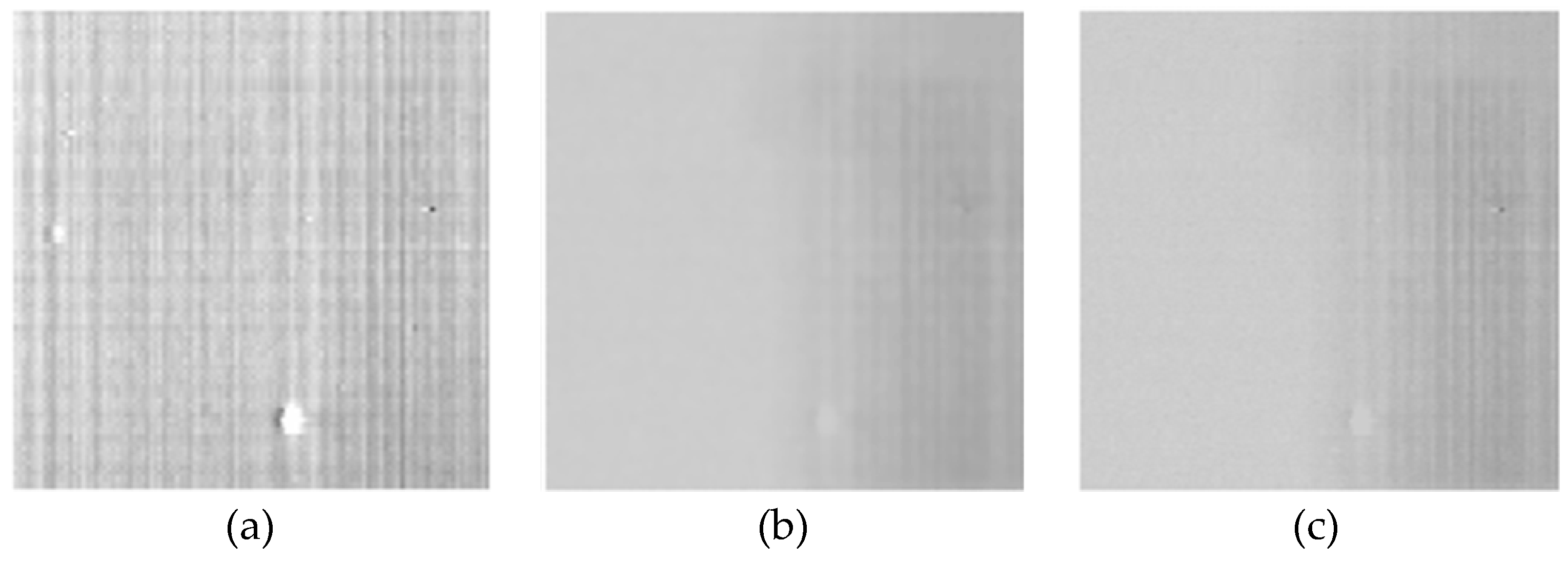
Example of nonuniformity with the two-point method (this image is of size 320 × 240 and was obtained by an uncooled infrared detector): (a) The source image, (b) the corrected image that was obtained via the two-point method, and (c) the corrected result that was obtained via the two-point method after 0.5 hours.
Figure 1.
Example of nonuniformity with the two-point method (this image is of size 320 × 240 and was obtained by an uncooled infrared detector): (a) The source image, (b) the corrected image that was obtained via the two-point method, and (c) the corrected result that was obtained via the two-point method after 0.5 hours.

Figure 2.
Gradient map and weighted map. (a1–a3) IR images with stripe nonuniformity. (b1–b3) Gradient maps of the original images. (c1–c3) 3D gradient maps of the original images. (d1–d3) Weighted maps of the original images that were obtained using the kernel function.
Figure 2.
Gradient map and weighted map. (a1–a3) IR images with stripe nonuniformity. (b1–b3) Gradient maps of the original images. (c1–c3) 3D gradient maps of the original images. (d1–d3) Weighted maps of the original images that were obtained using the kernel function.

Figure 3.
The curves of Kernel function.

Figure 4.
Results that were obtained by various filters. (a) The original image, (b) WGIF using our proposed weight map, (c) WGIF using the Sobel gradient operator weight (d) WGIF using the weight in [26] (e) GIF (f) GGIF.
Figure 4.
Results that were obtained by various filters. (a) The original image, (b) WGIF using our proposed weight map, (c) WGIF using the Sobel gradient operator weight (d) WGIF using the weight in [26] (e) GIF (f) GGIF.

Figure 5.
Schematic diagram of the proposed nonuniformity correction (NUC) method.

Figure 6.
Results of stripe nonuniformity estimation. (a1–a2) The original image, (b1–b2) the ideal image, and (c1–c2) the stripe nonuniformity image.
Figure 6.
Results of stripe nonuniformity estimation. (a1–a2) The original image, (b1–b2) the ideal image, and (c1–c2) the stripe nonuniformity image.

Figure 7.
Temporal profile of the estimated nonuniformity. (a) The estimated stripe nonuniformity sequence and (b) the temporal profile of two pixels in sequence.
Figure 7.
Temporal profile of the estimated nonuniformity. (a) The estimated stripe nonuniformity sequence and (b) the temporal profile of two pixels in sequence.

Figure 8.
Results of nonlinear diffusion equation filtering. (a) A pixel containing the nonuniformity and (b) a pixel containing the moving scene.
Figure 8.
Results of nonlinear diffusion equation filtering. (a) A pixel containing the nonuniformity and (b) a pixel containing the moving scene.

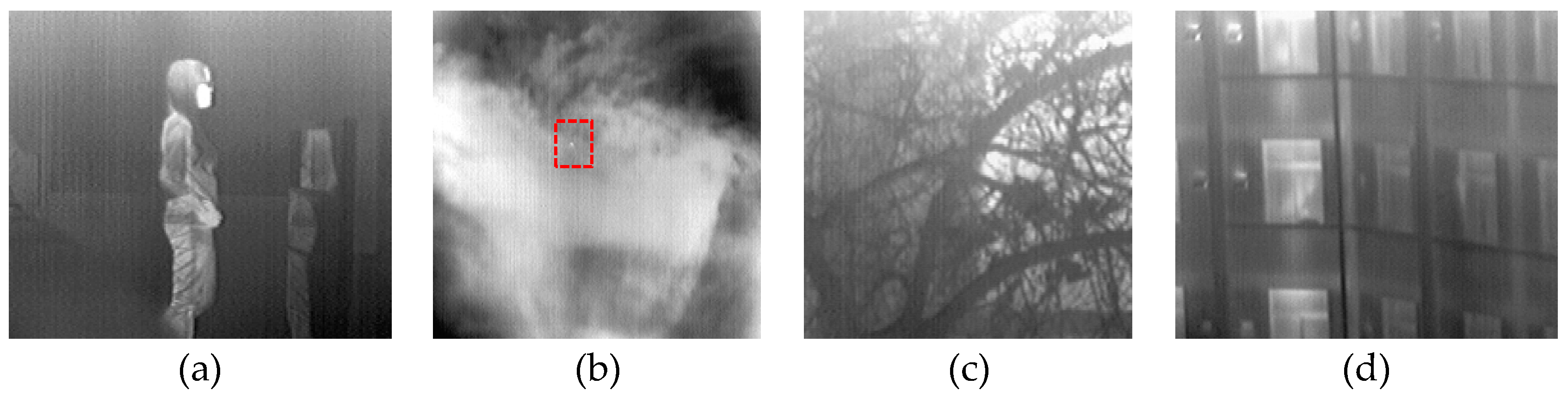
Figure 9.
Four raw IR image sequences for testing. (a) A walking girl, (b) a moving small target against a sky background, (c) a plant, and (d) windows.
Figure 9.
Four raw IR image sequences for testing. (a) A walking girl, (b) a moving small target against a sky background, (c) a plant, and (d) windows.

Figure 10.
NUC results that were obtained using various weights. (a1–a4) The original image, (b1–b4) the proposed weight, (c1–c4) the weight of [26], and (d1–d4) the Sobel weight.
Figure 10.
NUC results that were obtained using various weights. (a1–a4) The original image, (b1–b4) the proposed weight, (c1–c4) the weight of [26], and (d1–d4) the Sobel weight.

Figure 11.
Computing time of the proposed method with different weights.

Figure 12.
NUC results of five methods. (a1–a4) The original image, (b1–b4) the TVRNN NN result, (c1–c4) the BF-THPF result, (d1–d4) the MIRE result, (e1–e4) the CNN result, and (f1–f4) the result of the proposed method.
Figure 12.
NUC results of five methods. (a1–a4) The original image, (b1–b4) the TVRNN NN result, (c1–c4) the BF-THPF result, (d1–d4) the MIRE result, (e1–e4) the CNN result, and (f1–f4) the result of the proposed method.

Figure 13.
3D views of the NUC results. (a) BF-THPF and (b) the proposed method.

Figure 14.
Curves of roughness and nonuniformity for Sequence 1 and Sequence 2. (a1,a2) Nonuniformity and (b1,b2) roughness.
Figure 14.
Curves of roughness and nonuniformity for Sequence 1 and Sequence 2. (a1,a2) Nonuniformity and (b1,b2) roughness.


Table 1.
Parameter settings of different NUC methods.
| Method | Parameter Settings |
|---|---|
| BTHPF-NUC | The size of the filter window: D = 4; the two standard deviation parameters: σd = 7 and σr = 30; the time constant: T = 3 |
| TVRNN NN-NUC | The spatial average kernel size: 9 × 9; iterative step: |
| MIRE NUC | Regulation parameter: s = 1; the window size: 8 × s. |
| CNN NUC | Trained CNN in the literature [23] |
| Proposed method | wd = 5, σ1 = 0.003, σ2 = 10, r = 20, α = −0.8, and m = 10 |
Table 2.
Objective assessment of various methods.
| Method | The 100th Frame of Seq. 1 | The 50th Frame of Seq. 2 | The 50th Frame of Seq. 3 | The 200th Frame of Seq. 4 | ||||
|---|---|---|---|---|---|---|---|---|
| U/% | ρ/% | U/% | ρ/% | U/% | ρ/% | U/% | ρ/% | |
| Original image | 11.12 | 16.94 | 2.36 | 3.88 | 5.66 | 5.34 | 8.48 | 10.61 |
| BTHPF-NUC | 6.95 | 8.52 | 1.11 | 1.33 | 4.11 | 3.73 | 6.06 | 5.61 |
| TVRNN NN-NUC | 10.16 | 15.47 | 1.79 | 2.85 | 5.47 | 5.08 | 7.99 | 9.05 |
| MIRE NUC | 10.34 | 16.56 | 2.11 | 3.68 | 5.52 | 5.41 | 7.87 | 10.37 |
| CNN NUC | 11.47 | 17.62 | 2.25 | 3.87 | 5.58 | 5.33 | 8.51 | 10.83 |
| Proposed method | 6.53 | 3.61 | 0.91 | 0.56 | 3.72 | 1.55 | 5.91 | 1.66 |
© 2019 by the authors. Licensee MDPI, Basel, Switzerland. This article is an open access article distributed under the terms and conditions of the Creative Commons Attribution (CC BY) license (http://creativecommons.org/licenses/by/4.0/).
Share and Cite
MDPI and ACS Style
Li, J.; Qin, H.; Yan, X.; Zeng, Q.; Yang, T. Temporal-Spatial Nonlinear Filtering for Infrared Focal Plane Array Stripe Nonuniformity Correction. Symmetry 2019, 11, 673. https://doi.org/10.3390/sym11050673
AMA Style
Li J, Qin H, Yan X, Zeng Q, Yang T. Temporal-Spatial Nonlinear Filtering for Infrared Focal Plane Array Stripe Nonuniformity Correction. Symmetry. 2019; 11(5):673. https://doi.org/10.3390/sym11050673
Chicago/Turabian StyleLi, Jia, Hanlin Qin, Xiang Yan, Qingjie Zeng, and Tingwu Yang. 2019. "Temporal-Spatial Nonlinear Filtering for Infrared Focal Plane Array Stripe Nonuniformity Correction" Symmetry 11, no. 5: 673. https://doi.org/10.3390/sym11050673
Note that from the first issue of 2016, this journal uses article numbers instead of page numbers. See further details here.