A New Hybrid MCDM Model: Sustainable Supplier Selection in a Construction Company

Abstract

Sustainable development is one of the most important preconditions for preserving resources and balanced functioning of a complete supply chain in different areas. Taking into account the complexity of sustainable development and a supply chain, different decisions have to be made day-to-day, requiring the consideration of different parameters. One of the most important decisions in a sustainable supply chain is the selection of a sustainable supplier and, often the applied methodology is multi-criteria decision-making (MCDM). In this paper, a new hybrid MCDM model for evaluating and selecting suppliers in a sustainable supply chain for a construction company has been developed. The evaluation and selection of suppliers have been carried out on the basis of 21 criteria that belong to all aspects of sustainability. The determination of the weight values of criteria has been performed applying the full consistency method (FUCOM), while a new rough complex proportional assessment (COPRAS) method has been developed to evaluate the alternatives. The rough Dombi aggregator has been used for averaging in group decision-making while evaluating the significance of criteria and assessing the alternatives. The obtained results have been checked and confirmed using a sensitivity analysis that implies a four-phase procedure. In the first phase, the change of criteria weight was performed, while, in the second phase, rough additive ratio assessment (ARAS), rough weighted aggregated sum product assessment (WASPAS), rough simple additive weighting (SAW), and rough multi-attributive border approximation area comparison (MABAC) have been applied. The third phase involves changing the parameter ρ in the modeling of rough Dombi aggregator, and the fourth phase includes the calculation of Spearman’s correlation coefficient (SCC) that shows a high correlation of ranks.

1. Introduction

Sustainable engineering implies the execution of all processes and activities respecting all aspects of sustainability: economic, social, and environmental aspects. In addition, it is necessary to take into account the interactions and symmetry between them. This is confirmed by Hutchins et al. [1] according to whom it is necessary to define and understand the relationships that exist among aspects of sustainability and how they influence each other. In the last two decades, according to Vanalle et al. [2], companies around the world have been showing increasing concern about the impact of their operations on the environment, which arises as a result of pressure by legal regulations, customers, and competitors. Taking this into account, construction companies operate under great pressure due to their potentially negative impact on the environment and a complete, sustainable supply chain. In line with sustainability—that has become inevitability—and urgent need, supply chains are also changing, and their focus is no longer just on rationalizing costs, but also on environmental concerns. On this basis, sustainable supply chain management (SSCM) and green supply chain management (GSCM) have been established. The SSCM concept, according to Sen et al. [3], is an integrated approach that links economic and social thinking together with environmental awareness in traditional supply chain management. SSCM is based on the idea that in addition to constant monitoring of economic values, companies must consider environmental and social aspects, too. This implies that, in order to achieve sustainability, companies should solve environmental issues together with meeting social standards at all levels of supply chain [4], and at the same time, achieving certain economic effects. In order to achieve the effects of SSCM, according to Rabbani et al. [5], a large number of individual participants in a supply chain, starting from suppliers to top managers, have to take into account sustainable aspects. At the very beginning of the sustainability concept, according to Singh and Trivedi [6], the focus was mainly on environmental issues, and much less on social aspects, as it was thought that by managing and reducing negative impacts on the environment, companies would achieve competitive advantages. Nowadays, it is a different situation and, therefore, the evaluation and selection of suppliers based on an equal number of criteria by all aspects of sustainability has been performed in this paper.

This paper has several interrelated objectives. The first aim of this research refers to the development and detailed description of the algorithm of a new rough complex proportional assessment (COPRAS) method. The second aim that appears as a causal link to the previous one refers to the development of a new hybrid model which implies the integration of full consistency method (FUCOM), rough Dombi aggregator, and rough COPRAS method. The third aim of the paper is to popularize the FUCOM method, which contributes to the objective determination of weight criteria values, as well as to popularize the application of MCDM methods in integration with rough numbers.

After the introductory part, which explains the aims and motivation for this research, the paper consists of five more sections. The second section presents a two-phase procedure for reviewing the situation in the field. A review of MCDM methods in sustainable civil engineering and a review of MCDM methods for sustainable supplier selection are presented. The third part includes the developed methodology of this paper. At the beginning of the section, the process of research is presented with the contributions and advantages of this paper. Then, the FUCOM method is briefly explained in the first part, while the algorithm of the developed rough COPRAS method is elaborated and explained, in detail, in the second part. The fourth section describes a complete procedure for the selection of a sustainable supplier in a construction company. A detailed calculation for each step of the developed methodology is presented in order to make the model much more understandable to readers. The fifth section is a sensitivity analysis and discussion. The sensitivity analysis implies the already described four-phase procedure, followed by a discussion of the results obtained. In the sixth section, concluding observations with paper contributions and guidelines for future research are provided.

2. Literature Review

2.1. Review of MCDM Methods in Sustainable Civil Engineering

Formal decision-making methods can be used to help improve the overall sustainability of industries and organizations [7]. According to Zavadskas et al. [8], as sustainable development is becoming more relevant, more and more articles are being published related to sustainability in the field of construction. According to same authors, sustainable decision-making in civil engineering, construction, and building technology can be supported by fundamental scientific achievements and multi-criteria decision-making (MCDM) theories that, according to Mardani et al. [9], are widely used. In the field of construction, increasing attention is being paid to energy efficiency and smart buildings, and therefore it is necessary to go towards sustainability in the design and construction of facilities and infrastructure.

Construction is an area that interacts enormously with the natural environment. A large percentage of raw materials are obtained from the earth, and in their treatment, processing, and the construction of buildings, certain environmental pollution is inevitable. Lombera and Rojo [10] use the Spanish MIVES (in English, integrated value model for sustainable assessment) methodology to define criteria for the sustainability of industrial buildings and to select the optimum solution with regard to them. A similar study is presented in [11], where authors also use the MIVES method but in combination with Monte Carlo simulation, in order to assess the sustainability of concrete structures. De la Fuente et al. [12] also apply the MIVES methodology together with the analytic hierarchy process (AHP) method in order to reduce subjective human impact on the selection of sewage pipe material. The MIVES methodology is also used in [13] in assessing the sustainability of alternatives—the types of concrete and their reinforcement for application in tunnels. The problem of monitoring, repairing, and returning to the function of steel bridge structures is a major challenge for engineers, especially because it is necessary to make key decisions, and wrongly made decisions can be very costly. In order to exclude subjectivity in selecting alternatives, Rashidi et al. [14] presented the decision support system (DSS), within which the simplified AHP (S-AHP) method was used. S-AHP combines simple multi-attribute rating technique (SMART) and AHP method. The aim is to help engineers in planning the safety, functionality, and sustainability of steel bridge structures. Jia et al. [15] present a framework for the selection of bridge construction between the ABC (Accelerated Bridge Construction) method and conventional alternatives, using the technique for order of preference by similarity to ideal solution (TOPSIS) and fuzzy TOPSIS methods.

Formisano and Mazzolani [16] present a new procedure for the selection of the optimum solution for seismic retrofitting of existing buildings which involves the application of three MCDM methods: TOPSIS, elimination and choice expressing reality (ELECTRE), and VlšeKriterijumska Optimizacija i Kompromisno Rešenje (VIKOR). Terracciano et al. [17] selected cold-formed thin-walled steel structures for vertical reinforcement and energy retrofitting systems of existing masonry constructions using TOPSIS method. Šiožinytė et al. [18] apply the AHP and TOPSIS grey MCDM methods to select an optimum solution for modernizing traditional buildings. Khoshnava et al. [19] apply MCDM methods to select energy efficient, ecological, recyclable materials for building, with respect to the three pillars of sustainability. In order to evaluate 23 criteria in the selection of materials, they use the decision-making trial and evaluation laboratory (DEMATEL) hybrid MCDM method together with the fuzzy analytic network process (FANP). Akadiri et al. [20] use fuzzy extended AHP (FEAHP) in order to select sustainable building materials. In [21], the ANP method is used to select an environmentally friendly method for the construction of a highway, since it can have a great impact on the environment. Most systems for evaluating the sustainability of facilities take into account only the environmental aspect and the environmental impact. However, it is necessary to take into account all three basic principles of sustainability, and thus Raslanas et al. [22], in their work, develop a system for evaluating the sustainability of recreational facilities using the AHP method. MCDM tool, according to Kumar et al. [23], is becoming popular in the field of energy planning due to the flexibility it provides to the decision-makers to take decisions while considering all the criteria and objectives simultaneously. MULTIMOORA and TOPSIS are used in [24] for sustainable decision-making in the energy planning. The authors have concluded that hydro and solar power systems were identified as the most sustainable. A study performed in [25] deals with developing a sustainability assessment framework for assessing technologies for the treatment of urban sewage sludge based on the logarithmic fuzzy preference programming-based fuzzy analytic hierarchy process (LFPPFAHP) and extension theory. Salabun et al. [26] developed an MCDM model with COMET method for offshore wind farm localization. This method is also used in [27] for sustainable manufacturing and for solving the problem of the sustainable ammonium nitrate transport in [28].

2.2. Review of MCDM Methods for Sustainable Supplier Selection

The selection of suppliers is a constant process that requires the consideration of a certain number of criteria needed to make a decision on the selection of the most suitable suppliers [29,30,31]. According to Yazdani et al. [32], supplier evaluation and selection is a significant strategic decision for reducing operating costs and improving organizational competitiveness to develop business opportunities. Therefore, it is necessary to pay special attention to the selection of suppliers, including all aspects of sustainability.

The supplier selection, according to many authors, is one of the most demanding problems of sustainable supply chain management [33]. Fuzzy approach in combination with TOPSIS method is applied in [34] for assessing the sustainable performance of suppliers. In order to select suppliers in terms of sustainability, Dai and Blackhurst [35] present an integrated approach based on AHP and the quality function deployment (QFD) method. For the sustainable supplier selection, Azadnia et al. [36] propose an integrated approach that, in addition to the Fuzzy AHP method, is based on multi-objective mathematical programming, as well as on rule-based weighted fuzzy method. In [37], the assessment of sustainable supply chain management and the selection of suppliers are performed using grey theory in combination with the DEMATEL method, while Luthra et al. [38] present an integrated approach consisting of a combination of AHP and VIKOR method based on 22 criteria for all three aspects of sustainability. Sustainable supplier selection of raw materials in order to achieve sustainable development of the company is performed in [39], based on the fuzzy entropy–TOPSIS method. Hsu et al. [40] present a hybrid approach based on several MCDM methods in order to select suppliers in terms of carbon emissions. The evaluation of the supplier performance in the field of electronic industry in order to implement green supply chains is a topic of research in [41]. The authors use rough DEMATEL–ANP (R’AMATEL) in combination with rough multi-attribute ideal real comparative analysis (R’MAIRCA) method. Liu et al. [42] select the suppliers of fresh products using best worst method (BWM) and multi-objective optimization on the basis of the ratio analysis (MULTIMOORA) method. Kusi-Sarpong et al. [43] present a framework for ranking and selecting the criteria for sustainable innovations in supply chain management based on the BWM method. A quantitative assessment of the performance of a sustainable supply chain is presented in [44] based on fuzzy entropy and fuzzy Multi-Attribute Utility Theory (MAUT) methods. Das and Shaw [45] propose a model based on AHP and fuzzy TOPSIS method for selecting a sustainable supply chain, taking into account carbon emissions and various social factors. Luthra et al. [46] propose the application of Delphi and fuzzy DEMATEL methods for identifying and evaluating guidelines for the application information and communication technologies in sustainable initiatives in supply chains. In [47], a framework that identifies sustainable processes in supply chains for individual industries in India is presented. The ranking of industry branches is carried out using six fuzzy MCDM methods. Liou et al. [48] are proposed hybrid model consists of DEMATEL, ANP, and COPRAS-G methods for improving green supply chain management. They have used 12 criteria for supplier selection in the electronic industry, and provided a systemic analytical model for the improvement of parts of the supply chain management.

3. Methods

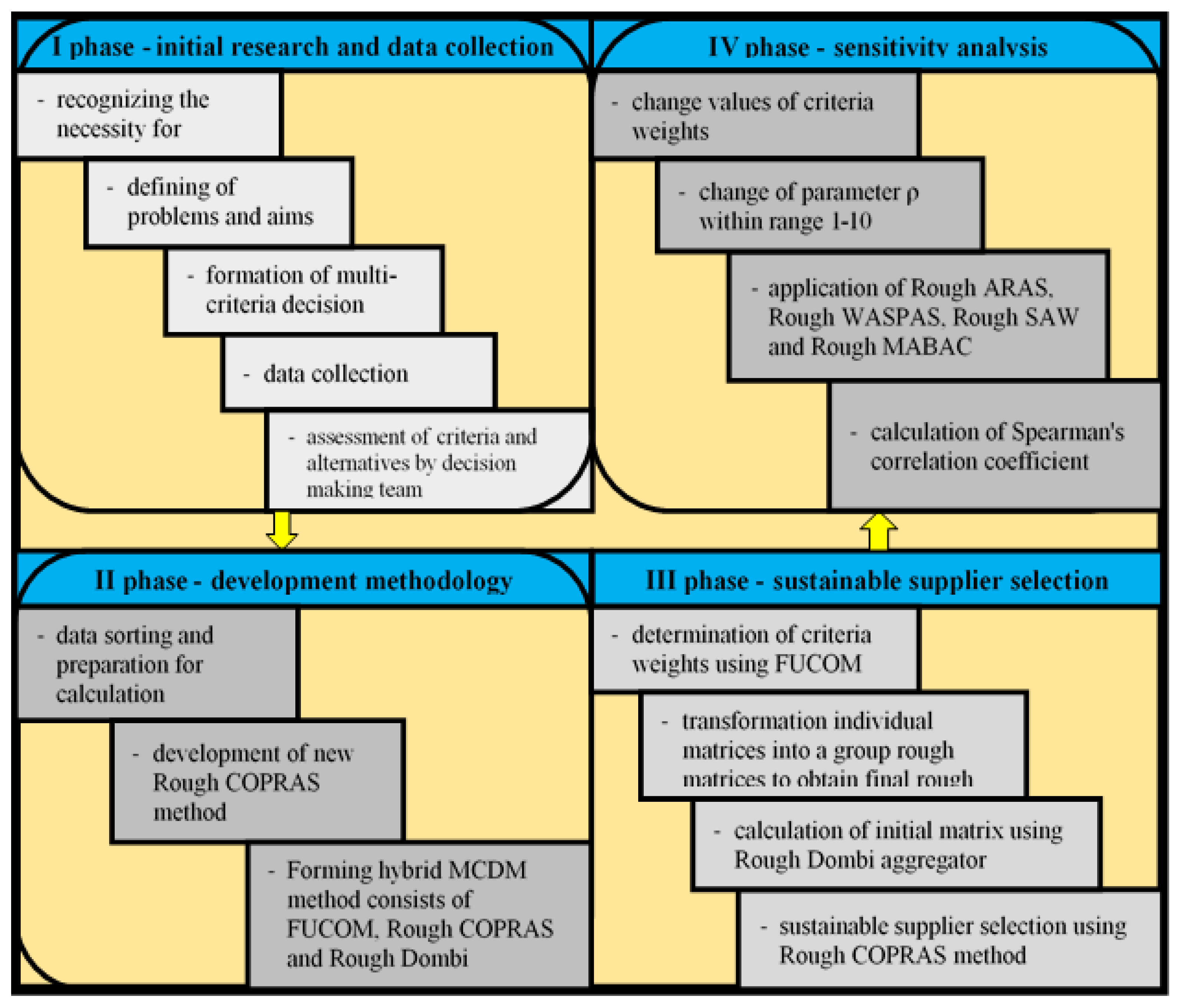
Figure 1 presents the methodology used in this paper, which consists of four phases:

• I—initial research and data collection
• II—developing methodology
• III—sustainable supplier selection
• IV—sensitivity analysis

The first phase consists of five steps. First, recognition of the need for this research and definition of the problems and aims of the research are performed in the first two steps, and the MCDM model is formed in the third step. After forming the model and defining all elements, the criteria, the alternatives, and the team of experts, the processes of data collection begins, which is the fourth step of the first phase. In the last step, the evaluation of the mutual significance of the criteria and evaluation of the alternatives by the formed team of experts are carried out. The second phase consists of three steps, where the first one is collected data sorting and preparation for their insertion into the developed model. The second step is the development and detailed description of the rough COPRAS method, and the creation of a hybrid MCDM model in the last step of this phase.

The third phase provides a detailed calculation for the evaluation and selection of a sustainable supplier, which consists of four steps. First, the determination of the criteria values using the FUCOM method is carried out, and then the transformation of the obtained values into rough numbers, in order to perform averaging using the rough Dombi aggregator and obtain the final values of the criteria. Subsequently, in the third step, the rough Dombi aggregator is again used to obtain an initial rough matrix, in order to make a decision on the selection of a sustainable supplier using the rough COPRAS method in the fourth step. The final phase is the sensitivity analysis already explained in the previous section.

We have decided to extent the COPRAS method with rough numbers from following reasons. Rough set theory is vague, subjective, and imprecise, while the COPRAS method, according to Mulliner et al. [49], allows for both benefit and cost criteria to be incorporated with one analysis without difficulty or question. The main advantage of COPRAS method compared with other MCDM methods is to be able to show utility degree. Also, COPRAS method has a simple procedure to use.

The following is a brief summary of the FUCOM method algorithm in the first part and the detailed algorithm description of rough COPRAS method in the second part.

3.1. Full Consistency Method (FUCOM)

The FUCOM method has been developed by Pamučar et al. [50] for determining the weights of criteria. It is a new method that, according to authors, represents a better method than AHP (analytical hierarchy process) and BWM (best worst method). So far, it has been applied in studies [51,52,53,54]. It consists of the following three steps:

Step 1. In the first step, the criteria from the predefined set of evaluation criteria $C=\left\{C_1,C_2,\dots ,C_n\right\}$ are ranked. The ranking is performed according to the significance of the criteria, i.e., starting from the criterion which is expected to have the highest weight coefficient to the criterion of the least significance.

$$C_{j\left(1\right)}>C_{j\left(2\right)}>\dots >C_{j\left(k\right)}$$

(1)

Step 2. In the second step, a comparison of the ranked criteria is carried out and the comparative priority (${\phi }_{k/\left(k+1\right)}$, $k=1,2,\dots ,n$, where k represents the rank of the criteria) of the evaluation criteria is determined.

$$\Phi =\left({\phi }_{1/2},{\phi }_{2/3},\dots ,{\phi }_{k/\left(k+1\right)}\right)$$

(2)

Step 3. In the third step, the final values of the weight coefficients of the evaluation criteria ${\left(w_1,w_2,\dots ,w_n\right)}^T$ are calculated. The final values of the weight coefficients should satisfy the two conditions:

(1)

that the ratio of the weight coefficients is equal to the comparative priority among the observed criteria (${\phi }_{k/\left(k+1\right)}$) defined in Step 2, i.e., that the following condition is met:

$$\frac{w_k}{w_{k+1}}={\phi }_{k/\left(k+1\right)}.$$

(3)

(2)

In addition to Condition (3), the final values of the weight coefficients should satisfy the condition of mathematical transitivity, i.e., that ${\phi }_{k/\left(k+1\right)}\otimes {\phi }_{\left(k+1\right)/\left(k+2\right)}={\phi }_{k/\left(k+2\right)}$.

Since ${\phi }_{k/\left(k+1\right)}=\frac{w_k}{w_{k+1}}$ and ${\phi }_{\left(k+1\right)/\left(k+2\right)}=\frac{w_{k+1}}{w_{k+2}}$, $\frac{w_k}{w_{k+1}}\otimes \frac{w_{k+1}}{w_{k+2}}=\frac{w_k}{w_{k+2}}$ is obtained.

Thus, another condition that the final values of the weight coefficients of the evaluation criteria need to meet is obtained, namely

$$\frac{w_k}{w_{k+2}}={\phi }_{k/\left(k+1\right)}\otimes {\phi }_{\left(k+1\right)/\left(k+2\right)}.$$

(4)

Based on the defined settings, the final model for determining the final values of the weight coefficients of the evaluation criteria can be defined.

$$\begin{array}{l}\begin{array}{cc}\min \chi & s.t.\end{array}\\ \begin{array}{cc}\left|\frac{w_{j\left(k\right)}}{w_{j\left(k+1\right)}}-{\phi }_{k/\left(k+1\right)}\right|\le \chi ,& \forall j\end{array}\\ \begin{array}{cc}\left|\frac{w_{j\left(k\right)}}{w_{j\left(k+2\right)}}-{\phi }_{k/\left(k+1\right)}\otimes {\phi }_{\left(k+1\right)/\left(k+2\right)}\right|\le \chi ,& \forall j\end{array}\\ \begin{array}{cc}{\displaystyle \sum _{j=1}^n{w}_j=1},& \forall j\end{array}\\ \begin{array}{cc}{w}_j\ge 0,& \forall j\end{array}.\end{array}$$

(5)

3.2. A Novel Rough COPRAS Method

The COPRAS method was expanded with rough numbers as part of a sensitivity analysis in the research [55]. So far, a complete algorithm that can enrich the theoretical field of multi-criteria decision-making has not been demonstrated. From this aspect, the algorithm presented below represents a significant contribution to the literature that addresses the problems of multi-criteria decision-making. It should be pointed out that the COPRAS method with interval rough numbers has been developed in [56], which differs from the proposed algorithm in this paper.

Rough COPRAS consists of the following steps:

Step 1: Forming a multi-criteria model. In the initial step, it is necessary to create a multi-criteria model with all necessary elements. Create a set of n alternatives that will be evaluated based on m criteria assessed by e experts.

Step 2: Forming an initial matrix for group decision-making (6). In this step, it is necessary to transform the individual matrices formed by experts’ evaluations into an initial group rough matrix. In order to achieve this, it is necessary to apply basic operations with rough numbers.

$$X={\begin{array}{cc}& \begin{array}{cccc}{C}_1& C_2& \dots & C_m\end{array}\\ \begin{array}{c}{A}_1\\ A_2\\ \dots \\ A_n\end{array}& \left[\begin{array}{cccc}RN\left(x_{11}\right)& RN\left(x_{12}\right)& \dots & RN\left(x_{1n}\right)\\ RN\left(x_{21}\right)& RN\left(x_{22}\right)& \dots & RN\left(x_{2n}\right)\\ \dots & \dots & \dots & \dots \\ RN\left(x_{m1}\right)& RN\left(x_{m2}\right)& \dots & RN\left(x_{mm}\right)\end{array}\right]\end{array}}_{m\times n},$$

(6)

where RN(x_ij) is an estimated value of the ith alternative in relation to the jth criterion, n is the number of alternatives, and m is the number of criteria.

Step 3: Normalization of the initial rough decision-making matrix applying the linear normalization procedure (7).

$$r_{ij}=\frac{x_{ij}^L;x_{ij}^U}{{\displaystyle \sum x_{ij}^l};x_{ij}^U}=\left[\frac{x_{ij}^L}{{\displaystyle \sum x_{ij}^U}};\frac{x_{ij}^U}{{\displaystyle \sum x_{ij}^L}}\right]$$

(7)

Step 4: Forming a weighted normalized matrix using the following Formula (8):

$$D=\left[d_{ij}^L;d_{ij}^U\right]=\left[w_J^L\times r_{ij}^L;w_J^U\times r_{ij}^U\right],$$

(8)

where $\left[r_{ij}^L;r_{ij}^U\right]$ is the normalized rough value of the ith alternative in relation to the jth criterion and w_j is the weight or significance of the jth criterion.

Step 5: In this step, it is necessary to calculate the sum of the weighted normalized values for both types of criteria, for benefit criteria using Equation (9):

$$S_{+i}={\left[s_{ij}^{+L};s_{ij}^{+U}\right]}_{1\times n},$$

(9)

and for cost criteria using Equation (10):

$$S_{-i}={\left[s_{ij}^{-L};s_{ij}^{-U}\right]}_{1\times n}.$$

(10)

Step 6: Determining the inverse summarized matrix for cost criteria (11):

$${\left(S_i^{-}\right)}^{-1}=\left[\frac{1}{s_{ij}^{-U}};\frac{1}{s_{ij}^{-L}}\right].$$

(11)

Step 7: Determining the sum of the matrix for cost criteria (12) and the sum of its inverse matrix (13) so that two matrices 1 × 1 are obtained:

$$\left(\overline{S_i^{-}}\right)={\displaystyle \sum {\left[s_i^{-L};s_i^{-U}\right]}_{1\times 1}},$$

(12)

$${\left(\overline{S_i^{-}}\right)}^{-1}={\displaystyle \sum {\left[\frac{1}{s_{ij}^{-U}};\frac{1}{s_{ij}^{-L}}\right]}_{1\times 1}}.$$

(13)

Step 8: Determining the relative significance for each alternative. The relative weight $Q_i$ for the ith alternative is calculated applying Equation (14):

$$Q_i=S_{+i}\times \frac{\left(\overline{S_i^{-}}\right)}{S_{-i}\times {\left(\overline{S_i^{-}}\right)}^{-1}}.$$

(14)

Step 9: Determining the priorities of alternatives. The priority in comparing the alternatives is identified on the basis of their relative weight, where the alternative with a higher relative weight value is given a higher priority or a rank, and the alternative with a maximum value represents the most acceptable alternative.

$$A^{*}=\left\{A_i|\underset{i}{\max Q_i}\right\}.$$

(15)

4. Case Study

Sustainable supplier selection in the construction company was carried out on the basis of 21 criteria shown and explained in

Table 1. Criteria for sustainable supplier selection.

Id	Criteria	References
C1	Economic criteria
C11	Costs/prices	The final cost to purchase a unit of raw or semi-finished product
C12	Quality	Quality is the degree to which a set of product characteristics meets customer requirements
C13	Delivery	The capability of transporting goods from a source location to a predefined destination
C14	Flexibility	Demand that can be profitably sustained, and time or cost required to add new products to existing production operations
C15	Technology capability	The sum of all the knowledge of an enterprise in support of technological innovation
C16	Financial ability	The capital needed to maintain normal business activities for an enterprise during a certain period of time
C17	Partnership relations	Determining the willingness to establish long-term and close business relations with suppliers to jointly develop the market
C2	Social criteria
C21	Reputation	Reputation marks the general opinion of the supplier, which relates to his reputation
C22	Safety and health at work	Concerned with the safety, health, and welfare of people at work
C23	Employees’ rights	A group of legal rights and claimed human rights having to do with labor relations between workers and their employers
C24	Local community influence	Neighboring relations between the company and the local government, the community, and all residents, representing the public image of the organization
C25	Training of employees	The process of enhancing the skills, capabilities, and knowledge of employees for a particular job
C26	Respect of rights and policies	Enterprises comply with all laws and regulations of the country, assume legal obligations, and promote good social public morals
C27	Disclosing information	Providing information to stakeholders about the materials used, carbon emissions, toxins released during production, etc.
C3	Environmental criteria
C31	Green image	The identity that consumers prioritize environmental conservation and sustainable business practices
C32	Environmental protection management system	A system that comprehensively evaluates the internal and external environmental performance of an organization
C33	Pollution control	The control of pollutants that are released into air, water, or soil
C34	Green products	Environmentally conscious products which are pollution-free, resource-saving, or renewable and recyclable
C35	ECO design	An approach to designing products with special consideration for the environmental impacts of the product during its whole lifecycle
C36	Consumption of resources	The use of non-renewable or, less often, renewable resources
C37	Green competences	The capacity to balance the containment relationships between economic and environmental performance

: economic, social, and environmental criteria. Each of these main criteria consists of seven subcriteria. The set of criteria used in this study was selected according to relevant literature, and based on interviews with authorized and managerial persons in the construction company. The first subcriterion that belongs to economic criteria C₁₁ (costs/prices) and the sixth subcriterion (consumption of resources) are the cost criteria, while the others are the benefit criteria.

In this study, the team of five experts took part in the process of determination of weight coefficients of criteria and assessment of alternatives. Experts with a minimum of six years’ experience in civil engineering were chosen. After interviewing the experts, the collected data were processed, and the aggregation of expert opinion was obtained. The collecting of data was carried out in the period from November 2018 until January 2019.

4.1. Determining Criteria Weights Using the FUCOM Method

In the following section, a detailed overview is provided of determining weight coefficients of the first-level criteria.

Step 1. In the first step, the decision-makers (DMs) ranked the criteria: DM₁: C₁ > C₃ > C₂; DM₂: C₁ > C₂ > C₃; DM₃: C₁ > C₃ > C₂; DM₄: C₃ > C₁ > C₂; and DM₅: C₁ > C₃ > C₂.

Step 2. In the second step, the decision-makers compared, in pairs, the ranked criteria from step 1. The comparison is made according to the first-ranked criterion, based on the above scale $\left[1,7\right]$. This is how the importance of the criteria is obtained (${\varpi }_{C_{j\left(k\right)}}$) for all the criteria ranked in step 1 (

Table 2. Significance of criteria.

DM1
Criteria	C1	C3	C2
$\mathrm{Significance}({\varpi }_{C_{j\left(k\right)}}$)	1	2.2	2.8
DM2
Criteria	C1	C2	C3
$\mathrm{Significance}({\varpi }_{C_{j\left(k\right)}}$)	1	2.7	2.7
DM3
Criteria	C1	C3	C2
$\mathrm{Significance}({\varpi }_{C_{j\left(k\right)}}$)	1	3.1	3.4
DM4
Criteria	C3	C1	C2
$\mathrm{Significance}({\varpi }_{C_{j\left(k\right)}}$)	1	1.7	2
DM5
Criteria	C1	C3	C2
$\mathrm{Significance}({\varpi }_{C_{j\left(k\right)}}$)	1	1.6	1.9

).

Based on the obtained significance of criteria, comparative significance values of criteria for each expert are calculated as follows:

$${\mathrm{DM}}_1:{\phi }_{C_1/C_3}=2.2/1=2.2,{\phi }_{C_3/C_2}=2.8/2.2=1.27;$$

$${\mathrm{DM}}_2:{\phi }_{C_1/C_2}=2.7/1=2.7,{\phi }_{C_2/C_3}=2.7/2.7=1;$$

$${\mathrm{DM}}_3:{\phi }_{C_1/C_3}=3.1/1=3.1,{\phi }_{C_3/C_2}=3.4/3.1=1.10;$$

$${\mathrm{DM}}_4:{\phi }_{C_3/C_1}=1.7/1=1.7,{\phi }_{C_1/C_2}=2/1.7=1.18;$$

$${\mathrm{DM}}_5:{\phi }_{C_1/C_3}=1.6/1=1.6,{\phi }_{C_3/C_2}=1.9/1.6=1.19.$$

Step 3. Final values of weight coefficient should satisfy two conditions:

(1)

Final values of weight coefficient should satisfy the condition where

$${\mathrm{DM}}_1:w_1/w_3=2.2,w_3/w_2=1.27;$$

$${\mathrm{DM}}_2:w_1/w_2=2.7,w_2/w_3=1;$$

$${\mathrm{DM}}_3:w_1/w_3=3.1,w_3/w_2=1.10;$$

$${\mathrm{DM}}_4:w_3/w_1=1.7,w_1/w_2=1.18;$$

$${\mathrm{DM}}_5:w_1/w_3=1.6,w_3/w_2=1.19.$$

(2)

In addition to the defined relations, final values of weight coefficients should satisfy also the condition of mathematical transitivity, $w_1/w_2=2.2\cdot 1.27=2.8$, $w_1/w_3=2.7\cdot 1=2.7$, $w_1/w_2=3.1\cdot 1.10=3.4$, $w_3/w_2=1.7\cdot 1.18=2$ and $w_1/w_2=1.6\cdot 1.19=1.9$.

By applying Expression (5), the models for determining weight coefficients of the first-level criteria for each decision-maker can be defined:

$$\begin{array}{l}{\mathrm{DM}}_1\left(\mathrm{First}\mathrm{level}\right)\\ \min \chi \\ s.t.\{\begin{array}{l}\begin{array}{cc}\left|\frac{w_1}{w_3}-2.2\right|=\chi ,& \left|\frac{w_3}{w_2}-1.27\right|=\chi ,\end{array}\\ \left|\frac{w_1}{w_2}-2.8\right|,\\ \begin{array}{cc}{\displaystyle \sum _{j=1}^3{w}_j=1},& \begin{array}{cc}{w}_j\ge 0,& \forall j\end{array}\end{array}\end{array}\end{array}\begin{array}{l}{\mathrm{DM}}_2\left(\mathrm{First}\mathrm{level}\right)\\ \min \chi \\ s.t.\{\begin{array}{l}\begin{array}{cc}\left|\frac{w_1}{w_2}-2.7\right|=\chi ,& \left|\frac{w_2}{w_3}-1\right|=\chi ,\end{array}\\ \left|\frac{w_1}{w_3}-2.7\right|,\\ \begin{array}{cc}{\displaystyle \sum _{j=1}^3{w}_j=1},& \begin{array}{cc}{w}_j\ge 0,& \forall j\end{array}\end{array}\end{array}\end{array}$$

$$\begin{array}{l}{\mathrm{DM}}_3\left(\mathrm{First}\mathrm{level}\right)\\ \min \chi \\ s.t.\{\begin{array}{l}\begin{array}{cc}\left|\frac{w_1}{w_3}-3.1\right|=\chi ,& \left|\frac{w_3}{w_2}-1.10\right|=\chi ,\end{array}\\ \left|\frac{w_1}{w_2}-3.4\right|,\\ \begin{array}{cc}{\displaystyle \sum _{j=1}^3{w}_j=1},& \begin{array}{cc}{w}_j\ge 0,& \forall j\end{array}\end{array}\end{array}\end{array}\begin{array}{l}{\mathrm{DM}}_4\left(\mathrm{First}\mathrm{level}\right)\\ \min \chi \\ s.t.\{\begin{array}{l}\begin{array}{cc}\left|\frac{w_3}{w_1}-1.7\right|=\chi ,& \left|\frac{w_1}{w_2}-1.18\right|=\chi ,\end{array}\\ \left|\frac{w_3}{w_2}-2\right|,\\ \begin{array}{cc}{\displaystyle \sum _{j=1}^3{w}_j=1},& \begin{array}{cc}{w}_j\ge 0,& \forall j\end{array}\end{array}\end{array}\end{array}$$

$$\begin{array}{l}{\mathrm{DM}}_5\left(\mathrm{First}\mathrm{level}\right)\\ \min \chi \\ s.t.\{\begin{array}{l}\begin{array}{cc}\left|\frac{w_1}{w_3}-1.6\right|=\chi ,& \left|\frac{w_3}{w_2}-1.19\right|=\chi ,\end{array}\\ \left|\frac{w_1}{w_2}-1.9\right|,\\ \begin{array}{cc}{\displaystyle \sum _{j=1}^3{w}_j=1},& \begin{array}{cc}{w}_j\ge 0,& \forall j\end{array}\end{array}\end{array}\end{array}$$

By solving the models presented, the values of weight coefficients for the first-level criteria for every decision-maker are obtained, as shown in

Table 3. Values of weight coefficients for the first level of decision-making according to each DM.

Id	DM1	DM2	DM3	DM4	DM5	Final Rough Values
C1	0.552	0.574	0.618	0.282	0.465	[0.394, 0.566]
C2	0.197	0.213	0.182	0.239	0.244	[0.199, 0.230]
C3	0.251	0.213	0.200	0.479	0.291	[0.228, 0.350]
DFC	0.0013	0.0000	0.0020	0.0015	0.0011	-

.

The final values shown in the last column of Table 3 are obtained by rough operations and the rough Dombi aggregator. First, the transformation of individual matrices into a group rough matrix is performed as follows:

$${\tilde{c}}_1=\left\{0.552,0.574,0.618,0.282,0.465\right\},$$

$$\begin{gathered} \underset{\_}{Lim}\left(0.552\right)=\frac{1}{3}\left(0.552+0.282+0.465\right)=0.433, \\ \overline{Lim}\left(0.552\right)=\frac{1}{3}\left(0.552+0.574+0.618\right)=0.581, \end{gathered}$$

$$\begin{gathered} \underset{\_}{Lim}\left(0.574\right)=\frac{1}{4}\left(0.552+0.574+0.282+0.465\right)=0.468, \\ \overline{Lim}\left(0.574\right)=\frac{1}{2}\left(0.574+0.618\right)=0.596, \end{gathered}$$

$$\begin{gathered} \underset{\_}{Lim}\left(0.618\right)=\frac{1}{5}\left(0.552+0.574+0.618+0.282+0.465\right)=0.498, \\ \overline{Lim}\left(0.618\right)=0.618, \end{gathered}$$

$$\begin{gathered} \underset{\_}{Lim}\left(0.282\right)=0.282, \\ \overline{Lim}\left(0.282\right)=\frac{1}{5}\left(0.552+0.574+0.618+0.282+0.465\right)=0.498, \end{gathered}$$

$$\begin{gathered} \underset{\_}{Lim}\left(0.465\right)=\frac{1}{2}\left(0.282+0.465\right)=0.373, \\ \overline{Lim}\left(0.465\right)=\frac{1}{4}\left(0.552+0.574+0.618+0.465\right)=0.552, \end{gathered}$$

$$\begin{gathered} RN\left(c_1^1\right)=\left[0.433,0.581\right];RN\left(c_1^2\right)=\left[0.468,0.596\right];RN\left(c_1^3\right)=\left[0.498,0.618\right]; \\ RN\left(c_1^4\right)=\left[0.282,0.498\right];RN\left(c_1^5\right)=\left[0.373,0.552\right]. \end{gathered}$$

Subsequently, the rough Dombi aggregator is applied and final rough values of the criteria at the first decision-making level are obtained. The aggregation is performed as follows.

After the transformation has been completed, five rough matrices, to which the operations of the rough Dombi aggregator is applied, are obtained. As mentioned in the previous part of the paper, the research has involved five experts who are assigned the same weight values of 0.200. Based on the presented values, Expression (8) from [56], and assuming that $\rho =1$ is at the position of C₁, the aggregation of values is performed as follows:

$$RNDWGA\left(c_1\right)=\{\begin{array}{l}\underset{\_}{Lim}\left(c_1\right)=\frac{{\displaystyle {\sum }_{j=1}^5\underset{\_}{Lim}\left({\phi }_j\right)}}{1+{\left\{{\displaystyle \sum _{j=1}^5{w}_j{\left(\frac{1-f\left(\underset{\_}{Lim}\left({\phi }_j\right)\right)}{f\left(\underset{\_}{Lim}\left({\phi }_j\right)\right)}\right)}^{\rho }}\right\}}^{1/\rho }}=\frac{2.052}{1+\left(0.200\times \left(\frac{1-0.210}{0.210}\right)+0.200\times \left(\frac{1-0.229}{0.229}\right)+\dots +0.200\times \left(\frac{1-0.180}{0.180}\right)\right)}=0.394\\ \overline{Lim}\left(c_1\right)=\frac{{\displaystyle {\sum }_{j=1}^5\overline{Lim}\left({\phi }_j\right)}}{1+{\left\{{\displaystyle \sum _{j=1}^5{w}_j{\left(\frac{1-f\left(\overline{Lim}\left({\phi }_j\right)\right)}{f\left(\overline{Lim}\left({\phi }_j\right)\right)}\right)}^{\rho }}\right\}}^{1/\rho }}=\frac{2.848}{1+\left(0.200\times \left(\frac{1-0.204}{0.204}\right)+0.200\times \left(\frac{1-0.211}{0.211}\right)+\dots +0.200\times \left(\frac{1-0.193}{0.193}\right)\right)}=0.567\end{array}.$$

Similarly, the decision-makers have ranked the criteria of the second level and the significance of criteria is obtained (

Table 4. The ranking and significance of the second-level criteria for a group of economic factors.

DM1
Economic factors	C11	C12	C13	C16	C14	C17	C15
${\varpi }_{C_{j\left(k\right)}}$	1	1.25	1.6	2.1	2.2	2.8	3.6
DM2
Economic factors	C12	C11	C16	C13	C14	C17	C15
${\varpi }_{C_{j\left(k\right)}}$	1	1.1	2.1	2.3	3.1	3.3	3.8
DM3
Economic factors	C11	C12	C13	C16	C14	C15	C17
${\varpi }_{C_{j\left(k\right)}}$	1	1	1.5	1.9	2.6	3.3	3.5
DM4
Economic factors	C12	C11	C13	C14	C16	C17	C15
${\varpi }_{C_{j\left(k\right)}}$	1	1.05	1.9	2.3	2.4	2.8	3.7
DM5
Economic factors	C12	C16	C11	C13	C14	C15	C17
${\varpi }_{C_{j\left(k\right)}}$	1	1.3	1.35	1.45	2	2.3	2.4

).

Based on the calculation, in the same way as with the criteria on the first level of decision-making, the calculation for the second decision-making level is made, and the values are shown in

Table 5. Values of weight coefficients for the second decision-making level according to each decision-maker for a group of economic criteria.

Id	DM1	DM2	DM3	DM4	DM5	Final Rough Values
C11	0.250	0.245	0.242	0.241	0.163	[0.203, 0.244]
C12	0.200	0.269	0.242	0.252	0.219	[0.219, 0.253]
C13	0.157	0.118	0.161	0.133	0.152	[0.131, 0.154]
C14	0.114	0.087	0.093	0.110	0.110	[0.095, 0.109]
C15	0.070	0.071	0.073	0.068	0.096	[0.071, 0.083]
C16	0.119	0.128	0.127	0.106	0.169	[0.117, 0.145]
C17	0.089	0.082	0.063	0.091	0.092	[0.074, 0.088]
DFC	0.0045	0.0005	0.0013	0.0017	0.0015	-

for a group of economic criteria, in

Table 6. The ranking and significance of the second-level criteria for a group of social factors.

DM1
Social factors	C22	C21	C26	C23	C27	C24	C25
${\varpi }_{C_{j\left(k\right)}}$	1	1.3	1.5	1.9	2.3	2.4	3
DM2
Social factors	C22	C21	C26	C24	C23	C27	C25
${\varpi }_{C_{j\left(k\right)}}$	1	1.15	1.8	2.1	2.6	2.85	3.2
DM3
Social factors	C21	C22	C26	C23	C24	C27	C25
${\varpi }_{C_{j\left(k\right)}}$	1	1	1.4	2.2	2.3	2.9	3.8
DM4
Social factors	C21	C22	C26	C23	C27	C24	C25
${\varpi }_{C_{j\left(k\right)}}$	1	1.2	1.55	2	2	2.1	2.7
DM5
Social factors	C22	C21	C26	C23	C27	C24	C25
${\varpi }_{C_{j\left(k\right)}}$	1	1.15	1.7	1.8	2.35	2.65	2.95

and

Table 7. Values of weight coefficients for the second decision-making level according to each decision-maker for a group of social criteria.

Id	DM1	DM2	DM3	DM4	DM5	Final Rough Values
C21	0.185	0.220	0.237	0.233	0.210	[0.204, 0.231]
C22	0.241	0.253	0.237	0.189	0.241	[0.216, 0.244]
C23	0.127	0.097	0.108	0.115	0.134	[0.107, 0.127]
C24	0.101	0.121	0.104	0.112	0.090	[0.100, 0.114]
C25	0.081	0.079	0.063	0.086	0.081	[0.074, 0.081]
C26	0.161	0.141	0.169	0.149	0.142	[0.144, 0.161]
C27	0.105	0.089	0.082	0.115	0.102	[0.090, 0.107]
DFC	0.0016	0.0022	0.0001	0.020	0.0013	-

for a group of social criteria, and in

Table 8. The ranking and significance of the second-level criteria for a group of environmental factors.

DM1
Environmental factors	C33	C35	C32	C31	C34	C36	C37
${\varpi }_{C_{j\left(k\right)}}$	1	1.2	1.3	1.75	2.2	2.7	3.6
DM2
Environmental factors	C33	C35	C31	C32	C36	C34	C37
${\varpi }_{C_{j\left(k\right)}}$	1	1.1	1.2	2.3	2.4	3.15	3.45
DM3
Environmental factors	C33	C35	C32	C31	C34	C36	C37
${\varpi }_{C_{j\left(k\right)}}$	1	1.4	1.7	2.1	2.2	2.7	2.8
DM4
Environmental factors	C35	C33	C32	C34	C36	C31	C37
${\varpi }_{C_{j\left(k\right)}}$	1	1.3	1.4	1.8	2.2	2.3	2.6
DM5
Environmental factors	C33	C35	C32	C31	C34	C36	C37
${\varpi }_{C_{j\left(k\right)}}$	1	1.2	1.5	1.6	2.4	2.7	3.2

and

Table 9. Values of weight coefficients for the second decision-making level according to each decision-maker for a group of environmental criteria.

Id	DM1	DM2	DM3	DM4	DM5	Final Rough Values
C31	0.134	0.198	0.121	0.101	0.147	[0.119, 0.161]
C32	0.180	0.103	0.148	0.165	0.158	[0.130, 0.165]
C33	0.234	0.238	0.252	0.178	0.237	[0.210, 0.242]
C34	0.106	0.076	0.115	0.128	0.098	[0.090, 0.115]
C35	0.195	0.216	0.180	0.231	0.197	[0.192, 0.214]
C36	0.086	0.099	0.094	0.105	0.088	[0.089, 0.099]
C37	0.065	0.069	0.090	0.091	0.074	[0.071, 0.086]
DFC	0.0012	0.0014	0.0017	0.0020	0.0014	-

for a group of environmental criteria.

Based on the significance of the groups of criteria (economic, social, and environmental) and applying Equation (5), the models for each decision-maker are formed. Solving these models, we obtain the values of weight coefficients per decision-makers (

Table 10. Final values of criteria.

Main criteria	Values of Main Criteria	Subcriteria	Values of Subcriteria	Final Weights
Economic	[0.203, 0.244]	w11	[0.203, 0.244]	[0.080, 0.138]
		w12	[0.219, 0.253]	[0.086, 0.144]
		w13	[0.131, 0.154]	[0.052, 0.087]
		w14	[0.095, 0.109]	[0.037, 0.062]
		w15	[0.071, 0.083]	[0.028, 0.047]
		w16	[0.117, 0.145]	[0.046, 0.082]
		w17	[0.074, 0.088]	[0.029, 0.050]
Social	[0.199, 0.230]	w21	[0.204, 0.231]	[0.041, 0.053]
		w22	[0.216, 0.244]	[0.043, 0.056]
		w23	[0.107, 0.127]	[0.021, 0.029]
		w24	[0.100, 0.114]	[0.020, 0.026]
		w25	[0.074, 0.081]	[0.015, 0.019]
		w26	[0.144, 0.161]	[0.029, 0.037]
		w27	[0.090, 0.107]	[0.018, 0.025]
Environmental	[0.228, 0.350]	w31	[0.119, 0.161]	[0.027, 0.057]
		w32	[0.130, 0.165]	[0.030, 0.058]
		w33	[0.210, 0.242]	[0.048, 0.085]
		w34	[0.090, 0.115]	[0.021, 0.040]
		w35	[0.192, 0.214]	[0.044, 0.075]
		w36	[0.089, 0.099]	[0.020, 0.035]
		w37	[0.071, 0.086]	[0.016, 0.030]

).

The final values of weight coefficients by all criteria are obtained by multiplying the weight coefficients of the main criteria with the subcriteria of the group to which they belong. As can be seen from Table 10, the most important criteria belong to the group of economic and then environmental criteria, which is understandable with regard to the area of existence of the company in which the research has been carried out.

4.2. Ranking Alternatives Using a New Rough COPRAS Method

Table 11. Comparison of alternatives by five decision-makers.

Id	A1					A2					A3					A4					A5
	E1	E2	E3	E4	E5	E1	E2	E3	E4	E5	E1	E2	E3	E4	E5	E1	E2	E3	E4	E5	E1	E2	E3	E4	E5
C11	3	2	3	2	3	4	3	2	3	2	3	3	1	2	2	5	4	3	4	4	6	3	3	4	3
C12	4	4	5	4	4	5	6	4	4	4	5	7	6	5	6	4	4	5	4	4	4	3	6	3	5
C13	5	5	4	4	4	3	5	5	3	3	5	5	6	5	5	3	4	4	4	4	6	4	4	4	4
C14	4	3	3	3	4	5	6	7	5	7	4	6	7	6	7	7	5	6	6	5	6	5	7	5	6
C15	4	6	4	5	3	5	6	5	5	5	5	6	6	5	6	6	5	5	6	5	7	5	5	5	5
C16	6	6	7	6	6	5	6	7	4	7	5	5	6	5	6	4	4	5	4	4	4	4	5	4	7
C17	5	4	4	3	5	5	7	6	5	6	5	6	6	6	6	6	4	6	6	4	7	4	6	4	6
C21	5	4	4	4	5	4	7	7	4	7	4	6	5	6	5	4	4	5	4	6	4	4	5	4	5
C22	5	3	3	3	5	5	6	6	4	7	5	6	5	7	5	4	4	6	4	4	4	4	5	4	7
C23	4	3	4	3	4	4	5	6	4	6	5	6	6	6	5	4	4	5	4	4	3	4	5	4	5
C24	4	4	4	4	4	5	5	6	5	6	4	5	6	5	6	6	4	5	5	4	5	4	5	4	5
C25	5	3	4	3	5	6	6	6	7	6	6	6	6	6	6	5	4	4	7	6	5	6	4	5	4
C26	5	2	2	3	5	5	5	6	5	7	4	5	6	5	6	4	4	4	4	4	5	4	4	4	3
C27	5	4	5	5	5	5	5	6	5	6	6	5	7	6	7	4	4	5	4	4	4	4	5	4	5
C31	5	3	4	3	5	4	6	7	6	7	6	5	7	5	7	5	5	6	3	5	5	5	6	7	6
C32	5	6	5	3	5	5	6	6	5	6	7	5	7	4	5	4	4	5	4	4	4	4	5	4	5
C33	4	3	5	3	4	6	6	7	6	7	7	5	7	5	7	6	5	5	4	5	4	5	5	5	5
C34	3	3	5	2	3	5	5	6	5	7	6	6	6	4	6	4	3	5	4	5	4	3	5	3	5
C35	4	4	5	4	4	5	6	6	5	6	6	6	6	6	6	4	4	5	4	4	4	4	5	3	5
C36	3	5	3	4	3	6	6	5	7	5	5	5	6	5	4	3	4	4	3	4	4	4	4	4	4
C37	5	3	4	4	5	5	5	6	5	5	7	5	6	5	4	6	4	5	6	4	6	4	5	4	5

presents the evaluation of alternatives according to all criteria based on the linguistic scale 1–7. In evaluating the alternatives, five decision-makers participated, whose expertise has already been described in the previous section.

In order to be able to apply the developed methodology, the transformation of individual matrices into a group rough matrix is performed first. An example of calculating the value of the third alternative according to criterion C₁₁ is given below:

$${\tilde{c}}_{11}=\left\{3,3,1,2,2\right\},$$

$$\begin{gathered} \underset{\_}{Lim}\left(3\right)=\frac{1}{5}\left(3+3+1+2+2\right)=2.2,\overline{Lim}\left(3\right)=3,\underset{\_}{Lim}\left(1\right)=1,\overline{Lim}\left(1\right)=\frac{1}{5}\left(3+3+1+2+2\right)=2.2, \\ \underset{\_}{Lim}\left(2\right)=\frac{1}{3}\left(1+2+2\right)=1.67,\overline{Lim}\left(2\right)=\frac{1}{4}\left(3+3+2+2\right)=2.5 \end{gathered}$$

$$RN\left(A_3^1\right)=RN\left(A_3^2\right)=\left[2.2,3\right];RN\left(A_3^3\right)=\left[1,2.2\right];RN\left(A_3^4\right)=RN\left(A_3^5\right)=\left[1.67,2.5\right].$$

Subsequently, the rough Dombi aggregator is applied and the final rough values of alternatives are obtained. The aggregation on the same example of the third alternative for criterion C₁₁ is carried out as follows:

$$RNDWGA\left(A_3\right)=\{\begin{array}{l}\underset{\_}{Lim}\left(A_3\right)=\frac{{\displaystyle {\sum }_{j=1}^5\underset{\_}{Lim}\left({\phi }_j\right)}}{1+{\left\{{\displaystyle \sum _{j=1}^5{w}_j{\left(\frac{1-f\left(\underset{\_}{Lim}\left({\phi }_j\right)\right)}{f\left(\underset{\_}{Lim}\left({\phi }_j\right)\right)}\right)}^{\rho }}\right\}}^{1/\rho }}=\frac{8.74}{1+\left(0.200\times \left(\frac{1-0.252}{0.252}\right)+0.200\times \left(\frac{1-0.252}{0.252}\right)+\dots +0.200\times \left(\frac{1-0.191}{0.191}\right)\right)}=1.609\\ \overline{Lim}\left(A_3\right)=\frac{{\displaystyle {\sum }_{j=1}^5\overline{Lim}\left({\phi }_j\right)}}{1+{\left\{{\displaystyle \sum _{j=1}^5{w}_j{\left(\frac{1-f\left(\overline{Lim}\left({\phi }_j\right)\right)}{f\left(\overline{Lim}\left({\phi }_j\right)\right)}\right)}^{\rho }}\right\}}^{1/\rho }}=\frac{13.2}{1+\left(0.200\times \left(\frac{1-0.227}{0.227}\right)+0.200\times \left(\frac{1-0.227}{0.227}\right)+\dots +0.200\times \left(\frac{1-0.189}{0.189}\right)\right)}=2.603\end{array}.$$

In the same way, other values for all alternatives are obtained according to all the criteria, which creates the initial aggregated matrix shown in

Table 12. Initial aggregated rough matrix.

Id	C11		C12		C21		C22		C23		C31
A1	2.321	2.826	4.038	4.339	4.151	4.622	3.276	4.204	3.333	3.830	3.408	4.488
A2	2.318	3.195	4.157	4.997	4.915	6.465	4.846	6.219	4.421	5.496	5.216	6.578
A3	1.609	2.603	5.342	6.222	4.704	5.623	5.160	6.007	5.344	5.833	5.429	6.502
A4	3.614	4.326	4.038	4.339	4.157	4.997	4.074	4.648	4.038	4.339	4.138	5.283
A5	3.183	4.325	3.397	4.880	4.151	4.622	4.189	5.350	3.691	4.619	5.342	6.222
∑	13.05	17.27	20.97	24.78	22.08	26.33	21.54	26.43	20.83	24.12	23.53	29.07

.

The summarized values for each criterion, which are necessary for the application of normalization in the next step, are shown in the last row of Table 12. Applying Equation (7), the normalized value for the third alternative according to criterion C₁₁ will be

$$r_{31}=\left[\frac{1.609}{17.27};\frac{2.603}{13.05}\right]=\left[0.09,0.20\right].$$

The last row of

Table 13. Normalized rough matrix.

Id	C11		C12		C21		C22		C23		C31
A1	0.13	0.22	0.16	0.21	0.16	0.21	0.12	0.20	0.14	0.18	0.12	0.19
A2	0.13	0.24	0.17	0.24	0.19	0.29	0.18	0.29	0.18	0.26	0.18	0.28
A3	0.09	0.20	0.22	0.30	0.18	0.25	0.20	0.28	0.22	0.28	0.19	0.28
A4	0.21	0.33	0.16	0.21	0.16	0.23	0.15	0.22	0.17	0.21	0.14	0.22
A5	0.18	0.33	0.14	0.23	0.16	0.21	0.16	0.25	0.15	0.22	0.18	0.26
wj	0.080	0.138	0.086	0.144	0.041	0.053	0.043	0.056	0.021	0.029	0.027	0.057

presents the values of the criteria obtained by applying the FUCOM method, which are necessary to create a weighted normalized matrix.

The fourth step is the weighting of normalized rough matrix (

Table 14. Weighted normalized rough matrix.

Id	C11		C12		C21		C22		C23		C31
A1	0.13	0.22	0.16	0.21	0.16	0.21	0.12	0.20	0.14	0.18	0.12	0.19
A2	0.13	0.24	0.17	0.24	0.19	0.29	0.18	0.29	0.18	0.26	0.18	0.28
A3	0.09	0.20	0.22	0.30	0.18	0.25	0.20	0.28	0.22	0.28	0.19	0.28
A4	0.21	0.33	0.16	0.21	0.16	0.23	0.15	0.22	0.17	0.21	0.14	0.22
A5	0.18	0.33	0.14	0.23	0.16	0.21	0.16	0.25	0.15	0.22	0.18	0.26

) by multiplying all the values of the normalized matrix with the weights of the criteria by applying Equation (8).

$$d_{31}=\left[0.09\times 0.08;0.02\times 0.138\right]=\left[0.007,0.028\right]$$

The next step is to summarize the values of the alternatives depending on the type of criteria, and two matrices are obtained. The first matrix refers to the sum of the values of alternatives according to the benefit group of criteria, while another one refers to cost criteria. In this research, cost criteria are C₁₁ and C₃₆.

The matrix for alternatives according to benefit criteria is

$$S_i^{+}=\left[\begin{array}{cc}0.096,& 0.215\\ 0.122,& 0.274\\ 0.131,& 0.285\\ 0.105,& 0.226\\ 0.104,& 0.240\end{array}\right].$$

An example of the calculation for the third alternative is

$$\begin{gathered} S_3^{L+}=\left[\begin{array}{l}0.019+0.011+0.007+0.005+0.008+0.006+0.007+0.008+0.005+0.004\\ +0.003+0.006+0.004+0.005+0.005+0.010+0.004+0.010+0.003\end{array}\right]=\left[0.131\right], \\ {S}_3^{U+}=\left[\begin{array}{l}0.043+0.023+0.017+0.011+0.019+0.012+0.014+0.016+0.008+0.007\\ +0.005+0.010+0.007+0.016+0.016+0.023+0.012+0.019+0.007\end{array}\right]=\left[0.285\right]. \end{gathered}$$

The matrix for alternatives according to cost criteria is

$$S_i^{-}=\left[\begin{array}{cc}0.014,& 0.037\\ 0.015,& 0.044\\ 0.011,& 0.037\\ 0.020,& 0.052\\ 0.018,& 0.053\end{array}\right].$$

An example of calculation is as follows:

$$S_3^{L-}=\left[0.007+0.004\right]=\left[0.011\right],$$

$$S_3^{U-}=\left[0.028+0.009\right]=\left[0.037\right].$$

After that, it is necessary to calculate the inverse values of the matrix $S_i^{-}$ by applying Equation (11), which is

$${\left(S_i^{-}\right)}^{-1}=\left[\begin{array}{cc}27.289,& 74.026\\ 22.553,& 64.948\\ 27.353,& 87.059\\ 19.137,& 50.864\\ 19.035,& 54.824\end{array}\right]$$

In the next step, it is first necessary to calculate the sum by column for cost criteria applying Equation (12), and the following values are obtained:

$$\left(\overline{S_i^{-}}\right)={\displaystyle \sum \left[s_i^{-L};s_i^{-U}\right]=\left[0.078,0.222\right]},$$

and then applying Equation (13) to calculate the sum for the inverse matrix, which will be

$${\left(\overline{S_i^{-}}\right)}^{-1}={\displaystyle \sum \left[\frac{1}{s_{ij}^{-U}};\frac{1}{s_{ij}^{-L}}\right]=\left[115.367,331.722\right]}.$$

In the next step, it is necessary to determine the relative significance for each alternative. The relative weight $Q_i$ by alternatives is

$$Q_i=\left[\begin{array}{cc}0.102,& 0.357\\ 0.127,& 0.399\\ 0.137,& 0.453\\ 0.109,& 0.324\\ 0.108,& 0.346\end{array}\right].$$

The ith alternative is calculated using Equation (14). An example of the calculation for the third alternative is

$$Q_3^L=S_{3+}^L+\frac{\left(\overline{S_3^{-L}}\right)}{S_{3-}^U\times {\left(\overline{S_3^{-U}}\right)}^{-1}}=0.131+\frac{0.078}{0.037\times 331.722}=0.137,$$

$$Q_3^U=S_{3+}^U+\frac{\left(\overline{S_3^{-U}}\right)}{S_{3-}^L\times {\left(\overline{S_3^{-L}}\right)}^{-1}}=0.285+\frac{0.222}{0.011\times 115.367}=0.453.$$

In the last step, the alternatives are ranked from the highest to the lowest value, and the results are as follows: A₃ > A₂ > A₁ > A₅ > A₄.

5. Sensitivity Analysis and Discussion

The sensitivity analysis has been performed throughout four phases, the first of which involves the creation of nine scenarios where the weights of criteria are modeled. The second phase involves the application of different methods, that is, comparative analysis, while the third phase implies the change of the parameter ρ into the values of 1–10. The fourth phase includes the application of Spearman’s correlation coefficient for the ranks of alternatives throughout the first two phases.

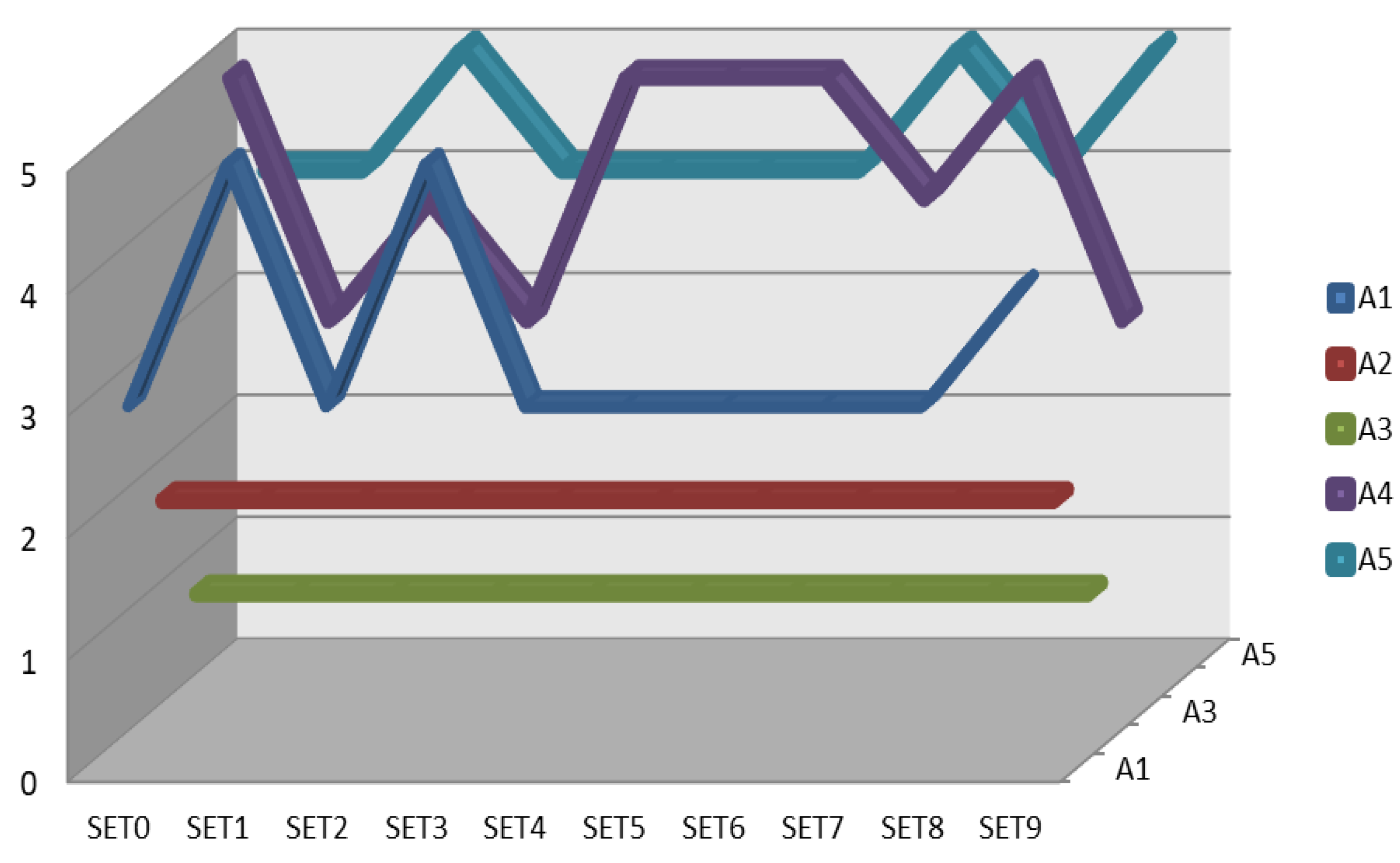
Figure 2 presents the ranks of alternatives throughout nine scenarios. The first scenario implies that all criteria are equally important, while in the second one, the six most important criteria (C₁₁, C₁₂, C₁₃, C₁₆, C₂₂, C₃₃) are reduced by 4%, and others are increased by 2%. In the third set, the six most important criteria are eliminated, and in the fourth one, the most important criteria are increased by 4%, while the rest are reduced by 2%. The fifth scenario involves the elimination of seven least important criteria (C₂₃, C₂₄, C₂₅, C₂₇, C₃₄, C₃₆, and C₃₇). In the sixth set, the criteria that belong to the economic group are reduced by 4%, while the criteria of the social group are proportionally increased. The values of environmental criteria remain unchanged. The seventh set implies a reverse situation from the aspect of economic and social criteria in relation to the sixth set. In the eighth scenario, decision-making is based only on economic criteria, and in the ninth scenario, only on environmental criteria.

The ranks of alternatives do not change in the fourth, fifth, sixth, and eighth criteria, which implies that the most important criteria play a very important role in the decision-making process in this research. This is confirmed by the fact that there are significant changes in the rankings in the first and third sets when all the criteria are equal, i.e., when the six most important ones are eliminated. In other scenarios there are no significant changes. It is important to emphasize that the two alternatives that represent the best solution, A₃ and A₂, do not change ranks in any scenario, which implies that they are insensitive to the changes in the significance of the criteria.

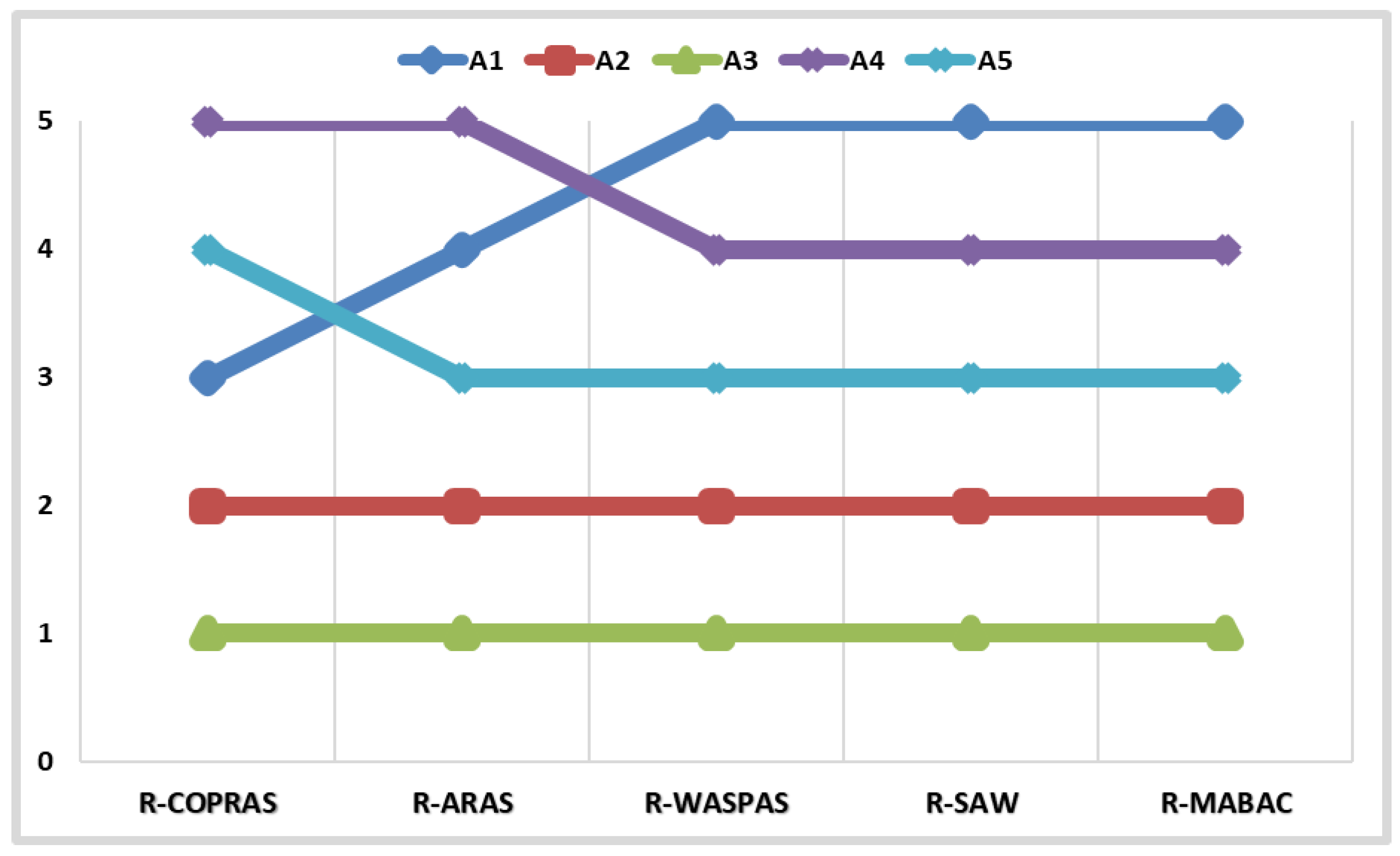
Figure 3 shows the comparison of the proposed model with other approaches developed recently: rough WASPAS [57], rough MABAC [58], rough SAW [59], and rough ARAS [60].

Observing the results obtained by other methods, the stability of the two best alternatives do not come into question, since they continue to take the first two positions using all the methods. The highest similarities of ranks obtained with rough COPRAS have the alternatives obtained with rough ARAS, where only the first and fifth alternatives change their positions. Slightly bigger changes in ranks are found with other methods.

Table 15. Ranks of alternatives depending on the change of parameter ρ.

Parameter ρ	Qi	Rank
ρ = 1	Q1 = 0.141; Q2 = 0.148; Q3 = 0.171; Q4 = 0.130; Q5 = 0.133	A3 > A2 > A1 > A5 > A4
ρ = 2	Q1 = 0.141; Q2 = 0.149; Q3 = 0.174; Q4 = 0.130; Q5 = 0.133	A3 > A2 > A1 > A5 > A4
ρ = 3	Q1 = 0.142; Q2 = 0.150; Q3 = 0.178; Q4 = 0.131; Q5 = 0.133	A3 > A2 > A1 > A5 > A4
ρ = 4	Q1 = 0.143; Q2 = 0.150; Q3 = 0.182; Q4 = 0.132; Q5 = 0.134	A3 > A2 > A1 > A5 > A4
ρ = 5	Q1 = 0.144; Q2 = 0.151; Q3 = 0.185; Q4 = 0.132; Q5 = 0.134	A3 > A2 > A1 > A5 > A4
ρ = 6	Q1 = 0.144; Q2 = 0.151; Q3 = 0.187; Q4 = 0.133; Q5 = 0.134	A3 > A2 > A1 > A5 > A4
ρ = 7	Q1 = 0.145; Q2 = 0.152; Q3 = 0.189; Q4 = 0.134; Q5 = 0.134	A3 > A2 > A1 > A5 = A4
ρ = 8	Q1 = 0.146; Q2 = 0.152; Q3 = 0.191; Q4 = 0.134; Q5 = 0.134	A3 > A2 > A1 > A5 = A4
ρ = 9	Q1 = 0.146; Q2 = 0.153; Q3 = 0.192; Q4 = 0.135; Q5 = 0.134	A3 > A2 > A1 > A5 > A4
ρ = 10	Q1 = 0.147; Q2 = 0.153; Q3 = 0.194; Q4 = 0.135; Q5 = 0.135	A3 > A2 > A1 > A5 = A4

presents the part of the sensitivity analysis that relates to the change of parameter ρ.

Changing the parameter ρ does not change significantly the initial results obtained. For the parameters ρ = 1–6, the same ranks are obtained as with the hybrid FUCOM–rough COPRAS model. The only changes in ranks are for parameters ρ = 7, ρ = 8, and ρ = 10 when the fourth and fifth alternative belongs to the same rank, and when ρ = 9, the fourth and fifth alternative change their positions while others remain unchanged. Based on the overall sensitivity analysis with the change of parameter ρ, it can be concluded that the model is not sensitive to these changes.

At the end of the sensitivity analysis, the calculated Spearman’s correlation coefficient for the first two phases is given (

Table 16. Spearman’s correlation coefficient for the first two phases of sensitivity analysis.

First Phase
SET	SET1	SET2	SET3	SET4	SET5	SET6	SET7	SET8	SET9	Average
SET0	0.600	0.900	0.600	1.000	1.000	1.000	0.900	1.000	0.700	0.856
Second Phase
Methods	R-COPRAS		R-ARAS		R-WASPAS		R-SAW		R-MABAC
R-COPRAS	1.000		0.900		0.700		0.700		0.700
R-ARAS			1.000		0.900		0.900		0.900
R-WASPAS					1.000		1.000		1.000
R-SAW							1.000		1.000
R-MABAC									1.000
Overall average									0.920

). For the third phase, calculation is not performed, since it is obvious that there is almost a complete correlation and, as already mentioned, the change of this parameter does not significantly affect the ranking of the alternatives.

Concerning the first phase of the sensitivity analysis in which the weights of the criteria change in sets, it can be seen that the model is sensitive to their changes. The initial set has a full correlation with four sets (4, 5, 6, and 8), while the smallest correlation SCC = 0.600 is with the first and third set, in which the ranks of two alternatives change for a total of three positions. In the second and seventh sets, the two last alternatives change positions between each other, so SCC = 0.900 with the initial set. In the ninth set, there is a change in the rank of three alternatives with SCC = 0.700. The total average value of SCC is 0.856, which represents a high correlation of ranks, regardless of the changes mentioned.

In the second phase, it can be observed that rough COPRAS has the highest correlation with the rough ARAS method of 0.900, while with other methods, rough WASPAS, rough SAW, and rough MABAC, SCC = 0.700. Taking this into account, it is concluded that rough WASPAS, rough SAW, and rough MABAC have a complete correlation, which ultimately implies that the average SCC = 0.920, which is a very high correlation of ranks.

6. Conclusions

This paper has proposed a new hybrid model that integrates FUCOM with the rough COPRAS method using the rough Dombi aggregator. This is the first time in the literature that this kind of model has been applied, that integrates the positive aspects of FUCOM method, rough set theory, rough Dombi aggregator for group decision-making, and the COPRAS method, which is one of the main contributions of this paper. In addition, the detailed and demonstrated algorithm of the rough COPRAS method also contributes to the overall field of multi-criteria decision-making.

Based on the 21 criteria of sustainability, a total of five suppliers in a construction company were considered, where it was concluded that the third and second suppliers are the best solutions regardless of any change in the model. This has been proven throughout a comprehensive sensitivity analysis in which different scenarios—with a change in the weight of criteria—were formed. The two mentioned alternatives are not sensitive to any changes in the values of the criteria. In addition, neither the change of parameter ρ, which is an integral part of the rough Dombi aggregator, affects the rankings of the third and second supplier, which has been confirmed by comparison with other approaches. The best solution in this model is completely insensitive, i.e., stable, while the ranks of other alternatives vary depending on the method of modeling the sensitivity analysis.

The developed model can be useful in other areas of engineering, but also when making real life decisions, since it adequately treats uncertainties by applying the theory of rough sets and subjectivity by applying the FUCOM method. Thus, it is possible to make more accurate and valid decisions that can have a huge impact on a sustainable supply chain. Future research related to this study will address the development and application of a similar model with the FUCOM method and an uncertainty theory, e.g., grey theory.

References

1. Hutchins, M.J.; Sutherland, J.W. An exploration of measures of social sustainability and their application to supply chain decisions. J. Clean. Prod. 2008, 16, 1688–1698. [Google Scholar] [CrossRef]
2. Vanalle, R.M.; Ganga, G.M.D.; Godinho Filho, M.; Lucato, W.C. Green supply chain management: An investigation of pressures, practices, and performance within the Brazilian automotive supply chain. J. Clean. Prod. 2017, 151, 250–259. [Google Scholar] [CrossRef]
3. Sen, D.K.; Datta, S.; Mahapatra, S.S. Sustainable supplier selection in intuitionistic fuzzy environment: A decision-making perspective. Benchmarking Int. J. 2018, 25, 545–574. [Google Scholar] [CrossRef]
4. Seuring, S. A review of modeling approaches for sustainable supply chain management. Decis. Support Syst. 2013, 54, 1513–1520. [Google Scholar] [CrossRef]
5. Rabbani, M.; Foroozesh, N.; Mousavi, S.M.; Farrokhi-Asl, H. Sustainable supplier selection by a new decision model based on interval-valued fuzzy sets and possibilistic statistical reference point systems under uncertainty. Int. J. Syst. Sci. Oper. Logist. 2017, 1–17. [Google Scholar] [CrossRef]
6. Singh, A.; Trivedi, A. Sustainable green supply chain management: trends and current practices. Compet. Rev. 2016, 26, 265–288. [Google Scholar] [CrossRef]
7. Zavadskas, E.K.; Govindan, K.; Antucheviciene, J.; Turskis, Z. Hybrid multiple criteria decision-making methods: A review of applications for sustainability issues. Econ. Res. Ekon. Istraživanja 2016, 29, 857–887. [Google Scholar] [CrossRef]
8. Zavadskas, E.; Antucheviciene, J.; Vilutiene, T.; Adeli, H. Sustainable decision-making in civil engineering, construction and building technology. Sustainability 2018, 10, 14. [Google Scholar] [CrossRef]
9. Mardani, A.; Jusoh, A.; Halicka, K.; Ejdys, J.; Magruk, A.; Ahmad, U.N. Determining the utility in management by using multi-criteria decision support tools: a review. Econ. Res. Ekon. Istraživanja 2018, 1–51. [Google Scholar] [CrossRef]
10. Lombera, J.T.S.; Rojo, J.C. Industrial building design stage based on a system approach to their environmental sustainability. Constr. Build. Mater. 2010, 24, 438–447. [Google Scholar] [CrossRef]
11. Del Cano, A.; Gomez, D.; de la Cruz, M.P. Uncertainty analysis in the sustainable design of concrete structures: A probabilistic method. Constr. Build. Mater. 2012, 37, 865–873. [Google Scholar] [CrossRef]
12. De la Fuente, A.; Pons, O.; Josa, A.; Aguado, A. Multi-Criteria Decision Making in the sustainability assessment of sewerage pipe systems. J. Clean. Prod. 2016, 112, 4762–4770. [Google Scholar] [CrossRef]
13. De la Fuente, A.; Blanco, A.; Armengou, J.; Aguado, A. Sustainability based-approach to determine the concrete type and reinforcement configuration of TBM tunnels linings. Case study: Extension line to Barcelona Airport T1. Tunn. Undergr. Space Technol. 2017, 61, 179–188. [Google Scholar] [CrossRef]
14. Rashidi, M.; Ghodrat, M.; Samali, B.; Kendall, B.; Zhang, C.W. Remedial Modelling of Steel Bridges through Application of Analytical Hierarchy Process (AHP). Appl. Sci. 2017, 7. [Google Scholar] [CrossRef]
15. Jia, J.M.; Ibrahim, M.; Hadi, M.; Orabi, W.; Xiao, Y. Multi-Criteria Evaluation Framework in Selection of Accelerated Bridge Construction (ABC) Method. Sustainability 2018, 10. [Google Scholar] [CrossRef]
16. Formisano, A.; Mazzolani, F.M. On the selection by MCDM methods of the optimal system for seismic retrofitting and vertical addition of existing buildings. Comput. Struct. 2015, 159, 1–13. [Google Scholar] [CrossRef]
17. Terracciano, G.; Di Lorenzo, G.; Formisano, A.; Landolfo, R. Cold-formed thin-walled steel structures as vertical addition and energetic retrofitting systems of existing masonry buildings. Eur. J. Environ. Civ. Eng. 2015, 19, 850–866. [Google Scholar] [CrossRef]
18. Siozinyte, E.; Antucheviciene, J.; Kutut, V. Upgrading the old vernacular building to contemporary norms: multiple criteria approach. J. Civ. Eng. Manag. 2014, 20, 291–298. [Google Scholar] [CrossRef]
19. Khoshnava, S.M.; Rostami, R.; Valipour, A.; Ismail, M.; Rahmat, A.R. Rank of green building material criteria based on the three pillars of sustainability using the hybrid multi criteria decision making method. J. Clean. Prod. 2018, 173, 82–99. [Google Scholar] [CrossRef]
20. Akadiri, P.O.; Olomolaiye, P.O.; Chinyio, E.A. Multi-criteria evaluation model for the selection of sustainable materials for building projects. Autom. Constr. 2013, 30, 113–125. [Google Scholar] [CrossRef]
21. Ozcan-Deniz, G.; Zhu, Y.M. A multi-objective decision-support model for selecting environmentally conscious highway construction methods. J. Civ. Eng. Manag. 2015, 21, 733–747. [Google Scholar] [CrossRef]
22. Raslanas, S.; Kliukas, R.; Stasiukynas, A. Sustainability assessment for recreational buildings. Civ. Eng. Environ. Syst. 2016, 33, 286–312. [Google Scholar] [CrossRef]
23. Kumar, A.; Sah, B.; Singh, A.R.; Deng, Y.; He, X.; Kumar, P.; Bansal, R.C. A review of multi criteria decision making (MCDM) towards sustainable renewable energy development. Renew. Sustain. Energy Rev. 2017, 69, 596–609. [Google Scholar] [CrossRef]
24. Streimikiene, D.; Balezentis, T.; Krisciukaitienė, I.; Balezentis, A. Prioritizing sustainable electricity production technologies: MCDM approach. Renew. Sustain. Energy Rev. 2012, 16, 3302–3311. [Google Scholar] [CrossRef]
25. An, D.; Xi, B.; Ren, J.; Ren, X.; Zhang, W.; Wang, Y.; Dong, L. Multi-criteria sustainability assessment of urban sludge treatment technologies: Method and case study. Resour. Conserv. Recycl. 2018, 128, 546–554. [Google Scholar] [CrossRef]
26. Sałabun, W.; Wątróbski, J.; Piegat, A. Identification of a multi-criteria model of location assessment for renewable energy sources. In Proceedings of the International Conference on Artificial Intelligence and Soft Computing, Zakopane, Poland, 12–16 June 2016; Springer: Cham, Switzerland, 2016; pp. 321–332. [Google Scholar]
27. Watróbski, J.; Sałabun, W. The characteristic objects method: A new intelligent decision support tool for sustainable manufacturing. In Proceedings of the International Conference on Sustainable Design and Manufacturing, Heraklion, Greece, 4–6 April 2016; pp. 349–359. [Google Scholar]
28. Wątróbski, J.; Sałabun, W.; Karczmarczyk, A.; Wolski, W. Sustainable decision-making using the COMET method: An empirical study of the ammonium nitrate transport management. In Proceedings of the 2017 Federated Conference on Computer Science and Information Systems (FedCSIS), Prague, Czech Republic, 3–6 September 2017; pp. 949–958. [Google Scholar]
29. Stević, Ž.; Vasiljević, M.; Puška, A.; Tanackov, I.; Junevičius, R.; Vesković, S. Evaluation of suppliers under uncertainty: a multiphase approach based on fuzzy AHP and fuzzy EDAS. Transport 2019, 34, 52–66. [Google Scholar] [CrossRef]
30. Badi, I.; Ballem, M. Supplier selection using the rough BWM-MAIRCA model: A case study in pharmaceutical supplying in Libya. Decis. Mak. Appl. Manag. Eng. 2018, 1, 16–33. [Google Scholar] [CrossRef]
31. Badi, I.; Abdulshahed, A.; Shetwan, A. A case study of supplier selection for steelmaking company in Libya by using Combinative Distance-based ASsessemnt (CODAS) model. Decis. Mak. Appl. Manag. Eng. 2018, 1, 1–12. [Google Scholar] [CrossRef]
32. Yazdani, M.; Chatterjee, P.; Zavadskas, E.K.; Zolfani, S.H. Integrated QFD-MCDM framework for green supplier selection. J. Clean. Prod. 2017, 142, 3728–3740. [Google Scholar] [CrossRef]
33. Keshavarz Ghorabaee, M.; Amiri, M.; Zavadskas, E.K.; Antucheviciene, J. Supplier evaluation and selection in fuzzy environments: A review of MADM approaches. Econ. Res. Ekon. Istraživanja 2017, 30, 1073–1118. [Google Scholar] [CrossRef]
34. Govindan, K.; Khodaverdi, R.; Jafarian, A. A fuzzy multi criteria approach for measuring sustainability performance of a supplier based on triple bottom line approach. J. Clean. Prod. 2013, 47, 345–354. [Google Scholar] [CrossRef]
35. Dai, J.; Blackhurst, J. A four-phase AHP-QFD approach for supplier assessment: a sustainability perspective. Int. J. Prod. Res. 2012, 50, 5474–5490. [Google Scholar] [CrossRef]
36. Azadnia, A.H.; Saman, M.Z.M.; Wong, K.Y. Sustainable supplier selection and order lot-sizing: an integrated multi-objective decision-making process. Int. J. Prod. Res. 2015, 53, 383–408. [Google Scholar] [CrossRef]
37. Su, C.M.; Horng, D.J.; Tseng, M.L.; Chiu, A.S.F.; Wu, K.J.; Chen, H.P. Improving sustainable supply chain management using a novel hierarchical grey-DEMATEL approach. J. Clean. Prod. 2016, 134, 469–481. [Google Scholar] [CrossRef]
38. Luthra, S.; Govindan, K.; Kannan, D.; Mangla, S.K.; Garg, C.P. An integrated framework for sustainable supplier selection and evaluation in supply chains. J. Clean. Prod. 2017, 140, 1686–1698. [Google Scholar] [CrossRef]
39. Zhao, H.R.; Guo, S. Selecting Green Supplier of Thermal Power Equipment by Using a Hybrid MCDM Method for Sustainability. Sustainability 2014, 6, 217–235. [Google Scholar] [CrossRef]
40. Hsu, C.W.; Kuo, T.C.; Shyu, G.S.; Chen, P.S. Low Carbon Supplier Selection in the Hotel Industry. Sustainability 2014, 6, 2658–2684. [Google Scholar] [CrossRef]
41. Chatterjee, K.; Pamucar, D.; Zavadskas, E.K. Evaluating the performance of suppliers based on using the R'AMATEL-MAIRCA method for green supply chain implementation in electronics industry. J. Clean. Prod. 2018, 184, 101–129. [Google Scholar] [CrossRef]
42. Liu, A.J.; Xiao, Y.X.; Ji, X.H.; Wang, K.; Tsai, S.B.; Lu, H.; Cheng, J.S.; Lai, X.J.; Wang, J.T. A Novel Two-Stage Integrated Model for Supplier Selection of Green Fresh Product. Sustainability 2018, 10. [Google Scholar] [CrossRef]
43. Kusi-Sarpong, S.; Gupta, H.; Sarkis, J. A supply chain sustainability innovation framework and evaluation methodology. Int. J. Prod. Res. 2018, 6, 1–9. [Google Scholar] [CrossRef]
44. Erol, I.; Sencer, S.; Sari, R. A new fuzzy multi-criteria framework for measuring sustainability performance of a supply chain. Ecol. Econ. 2011, 70, 1088–1100. [Google Scholar] [CrossRef]
45. Das, R.; Shaw, K. Uncertain supply chain network design considering carbon footprint and social factors using two-stage approach. Clean Technol. Environ. Policy 2017, 19, 2491–2519. [Google Scholar] [CrossRef]
46. Luthra, S.; Mangla, S.K.; Chan, F.T.S.; Venkatesh, V.G. Evaluating the Drivers to Information and Communication Technology for Effective Sustainability Initiatives in Supply Chains. Int. J. Inf. Technol. Decis. Mak. 2018, 17, 311–338. [Google Scholar] [CrossRef]
47. Padhi, S.S.; Pati, R.K.; Rajeev, A. Framework for selecting sustainable supply chain processes and industries using an integrated approach. J. Clean. Prod. 2018, 184, 969–984. [Google Scholar] [CrossRef]
48. Liou, J.J.; Tamošaitienė, J.; Zavadskas, E.K.; Tzeng, G.H. New hybrid COPRAS-G MADM Model for improving and selecting suppliers in green supply chain management. Int. J. Prod. Res. 2016, 54, 114–134. [Google Scholar] [CrossRef]
49. Mulliner, E.; Malys, N.; Maliene, V. Comparative analysis of MCDM methods for the assessment of sustainable housing affordability. Omega 2016, 59, 146–156. [Google Scholar] [CrossRef]
50. Pamučar, D.; Stević, Ž.; Sremac, S. A new model for determining weight coefficients of criteria in mcdm models: Full consistency method (fucom). Symmetry 2018, 10, 393. [Google Scholar] [CrossRef]
51. Nunić, Z.B. Evaluation and selection of Manufacturer PVC carpentry using FUCOM-MABAC model. Oper. Res. Eng. Sci. Theory Appl. 2018, 1, 13–28. [Google Scholar] [CrossRef]
52. Zavadskas, E.K.; Nunić, Z.; Stjepanović, Ž.; Prentkovskis, O. A novel rough range of value method (R-ROV) for selecting automatically guided vehicles (AGVs). Stud. Inform. Control 2018, 27, 385–394. [Google Scholar] [CrossRef]
53. Pamučar, D.; Lukovac, V.; Božanić, D.; Komazec, N. Multi-criteria FUCOM-MAIRCA model for the evaluation of level crossings: case study in the Republic of Serbia. Oper. Res. Eng. Sci. Theory Appl. 2018, 1, 108–129. [Google Scholar] [CrossRef]
54. Prentkovskis, O.; Erceg, Ž.; Stević, Ž.; Tanackov, I.; Vasiljević, M.; Gavranović, M. A New Methodology for Improving Service Quality Measurement: Delphi-FUCOM-SERVQUAL Model. Symmetry 2018, 10, 757. [Google Scholar] [CrossRef]
55. Stević, Ž.; Pamučar, D.; Vasiljević, M.; Stojić, G.; Korica, S. Novel integrated multi-criteria model for supplier selection: Case study construction company. Symmetry 2017, 9, 279. [Google Scholar] [CrossRef]
56. Pamučar, D.; Božanić, D.; Lukovac, V.; Komazec, N. Normalized weighted geometric bonferroni mean operator of interval rough numbers-application in interval rough DEMATEL-COPRAS model. Facta Univ. Ser. Mech. Eng. 2018, 16. [Google Scholar] [CrossRef]
57. Stojić, G.; Stević, Ž.; Antuchevičienė, J.; Pamučar, D.; Vasiljević, M. A Novel Rough WASPAS Approach for Supplier Selection in a Company Manufacturing PVC Carpentry Products. Information 2018, 9, 121. [Google Scholar] [CrossRef]
58. Roy, J.; Chatterjee, K.; Bandhopadhyay, A.; Kar, S. Evaluation and selection of Medical Tourism sites: A rough AHP based MABAC approach. arXiv 2016, arXiv:1606.08962. [Google Scholar]
59. Stević, Ž.; Pamučar, D.; Zavadskas, E.K.; Ćirović, G.; Prentkovskis, O. The Selection of Wagons for the Internal Transport of a Logistics Company: A Novel Approach Based on Rough BWM and Rough SAW Methods. Symmetry 2017, 9, 264. [Google Scholar] [CrossRef]
60. Radović, D.; Stević, Ž.; Pamučar, D.; Zavadskas, E.; Badi, I.; Antuchevičiene, J.; Turskis, Z. Measuring performance in transportation companies in developing countries: a novel rough ARAS model. Symmetry 2018, 10, 434. [Google Scholar] [CrossRef]
Figure 1. Research flow with proposed model.
Symmetry 11 00353 g001
Figure 2. Sensitivity analysis by changing the weight values of criteria.
Symmetry 11 00353 g002
Figure 3. Comparison of the results of the developed model with other methods.
Symmetry 11 00353 g003