Adaptive Sub-Nyquist Spectrum Sensing for Ultra-Wideband Communication Systems ^†

Abstract

With the ever-increasing demand for high-speed wireless data transmission, ultra-wideband spectrum sensing is critical to support the cognitive communication over an ultra-wide frequency band for ultra-wideband communication systems. However, it is challenging for the analog-to-digital converter design to fulfill the Nyquist rate for an ultra-wideband frequency band. Therefore, we explore the spectrum sensing mechanism based on the sub-Nyquist sampling and conduct extensive experiments to investigate the influence of sampling rate, bandwidth resolution and the signal-to-noise ratio on the accuracy of sub-Nyquist spectrum sensing. Afterward, an adaptive policy is proposed to determine the optimal sampling rate, and bandwidth resolution when the spectrum occupation or the strength of the existing signals is changed. The performance of the policy is verified by simulations.

1. Introduction

After decades of rapid development, wireless technologies have been intensively applied to almost every field from daily communications to mobile medical and battlefield communications. Whether you admit it or not, wireless communication technologies have become an essential part of our daily life. According to the global mobile data traffic forecast report [1] by Cisco, the expected overall mobile data traffic will be 77 exabytes per month by 2022, almost a 4-fold increase over that in 2018. As a result of the ever-increasing demand for higher speed wireless communication, more and more spectrum will be consumed in the near future.

In terms of the Shannon theorem: $C=Wlog(1+\frac{S}{N})$ (where C refers to communication capacity, S stands for signal, N refers to noise.), the communication capacity depends on the bandwidth and the signal-to-noise ratio (SNR).

The required bandwidth increases in pace with the growth of wireless transmission rate. For example, from 802.11ac to 802.11ad, though the transmission rate increases from 1.35 Gbps to 7 Gbps, the corresponding bandwidth consumed also increases from 160 MHz to 2160 MHz. In 2013, Koenig achieved 100 Gbps wireless transmission rate with a 35 GHz band at the sub-THz frequency [2] using their customized communication system. The fact that advances in wireless technologies rely on the spectrum resource makes spectrum very scarce and precious.

Despite the fact that we can use a wide range of wireless spectrum from 3 Hz to 3000 GHz, most of the spectrum has been already allocated to specific organization. However, in terms of current licensed users, the spectrum utilization remains low and a large mount of spectrum is still underutilized [3]. To handle this man-made spectrum scarcity [4], cognitive radio (CR) technology is proposed. In a cognitive network, when the licensed spectrum is underutilized by the licensed users (primary users, PUs), unlicensed users (secondary users, SUs) can utilize the licensed spectrum. With cognitive radio technologies, we can expand current transmission to unoccupied frequency bands to get a broader transmission bandwidth. In fact, Qualcomm and many other companies have already proposed such a solution to 4G LTE, which is called LTE-U (LTE in unlicensed spectrum) [5]. LTE-U can use the 4G LTE radio communication technology in unlicensed spectrum, for example, the 5 GHz band used by dual-band Wi-Fi equipment. LTE-U can not only greatly increase the LTE transmission rate but also highly improve the spectrum efficiency.

With the purpose of finding more available spectrum resource, SUs take advantages of the spectrum sensing process to detect the occupation condition of a spectrum segment. As with cognitive networks, spectrum sensing is fundamental and crucial. Many algorithms, including matched filtering [6], energy detection [7], and cyclostationary feature detection [8], are proposed to deal with spectrum sensing. However, most of the researchers pay attention to the sensing of a narrowband frequency range. To satisfy the ever-increasing transmission demand, only when we search across an ultra-wideband spectrum range can we find out enough available spectrum for communication. As a result, traditional narrow band spectrum sensing technologies are incapable of sensing in an ultra-wideband communication system. The ability to perform ultra-wideband spectrum sensing is essential to future communication systems.

However, there are many challenges to conduct the ultra-wideband spectrum sensing with the Nyquist sampling rate, i.e., the sampling rates are at least twice the bandwidth of the signal. In ultra-wideband communication systems, several GHz or an even larger spectrum is utilized to handle high transmission rate. For example, in Koenig’s [2] system, the related sampling rate should be 70 GHz or higher, which is arduous to carry out. On one hand, it is almost impossible to implement such a high speed analog-to-digital converter (ADC). On the other hand, even if we can produce such a high speed ADC, the fact that it is expensive and energy-consuming makes it unable to deploy on mobile devices.

Can we just deal with the ultra-wideband spectrum sensing using undersampled data whose sampling rate is less than the Nyquist rate? In fact, as early as 20 years ago, Xia [9] proposed an algorithm to recover a high frequency from its undersampled data. During the past several years, many researchers devoted themselves to it. In 2014, Hassanieh et al. [10] propose a wideband spectrum sensing method using a sparse FFT algorithm with sub-Nyquist sampling rates. Though sub-Nyquist sensing technologies are promising, there are more challenges.

Main Challenges. The main challenge to handle ultra-wideband spectrum sensing with sub-Nyquist sampling rates is the information loss resulting from the sub-Nyquist sampling, which makes us unable to recover the frequency information from the sampled data. That is, we cannot infer the frequency occupancy status from the undersampled data. There are two main reasons that cause information loss.

Spectrum Leakage. We usually use a finite set of samples to compute the energy of the signal. However, to the discrete Fourier transformation (DFT) process, the sampled signals are treated as periodic in time. Consequently, the signals we use for DFT are actually:

$$x_N\left(n\right)=x\left(n\right)w\left(n\right),$$

(1)

where $x_N\left(n\right)$ is truncated from $x\left(n\right)$. $w\left(n\right)$ is a windowing function. Since only the finite N points are used, $w\left(n\right)$ can be regarded as a rectangular window.

We can evaluate the consequence of truncating by transforming $x_N\left(n\right)$ into the frequency domain:

$$X_N\left(\omega \right)=X\left(\omega \right)\ast W\left(\omega \right).$$

(2)

$W\left(\omega \right)$ is a $sinc$ function. Its sidelobes result in non-zero values in the vicinity frequencies of $X_N\left(\omega \right)$, thus making spectrum leakage happen.

Aliasing Effect. When the sampling rate is lower than the Nyquist rate, i.e.: $f_s<2W$ ($f_s$ is the sampling rate and W is the bandwidth of the signal), aliasing happens. Just as Figure 1 shows, high frequencies and lower frequencies overlap when aliasing occurs.

Previous study on sub-Nyquist sensing, including compressed sensing and several other works, mainly focuses on designing different sampling modes, which allow frequencies to be recovered from the undersampled data. However, most of the systems are very complex and are strict with time synchronization. They try to reconstruct the whole signal and then detect the spectrum occupancy, thus leading to huge computation and energy-consuming. Actually, in terms of spectrum sensing, there is little need to recover the whole signal. We only need to reconstruct the frequencies we are interested in.

Based on these considerations, this paper introduces SNSS (Sub-Nyquist Spectrum Sensing) to address this problem. SNSS makes full use of the Chinese Remainder Theorem (CRT) to recover all the frequency information that we are interested in from the undersampled data, thus making it possible to sense the ultra-wideband spectrum with relatively low sampling rates and computing resources. Unlike the previous algorithm, SNSS conducts energy detection directly on the aliased data and then reconstruct the frequency occupancy status. SNSS can simplify the system architecture and reduce the computation amount.

Additionally, the spectrum usage in a modern wireless communication system is time-varying in practice, i.e., an idle spectrum segment becomes unavailable immediately when the PU is active. To provide efficient cognitive communication, spectrum sensing should be sensitive to the change of spectrum occupancy. Besides, the signal strength at a given frequency band is time-varying. For example, when the PU is mobile, the signal observed at a static position varies persistently. It is critical to keep tracking the PU’s behavior even when the signal from the PU is weak. However, the implementation of most sub-Nyquist spectrum sensing methods do not take into account the effects of network dynamics. In fact, when the behaviors of PUs change, they cannot adjust the runtime parameters to adapt to the varying conditions. Based on these observations, this paper proposes ASNSS (Adaptive Sub-Nyquist Spectrum Sensing) to deal with the dynamics.

The contributions of this paper are as below.

• We propose SNSS, which can determine the occupancy status of the spectrum from multiple sub-sampled data. Taking advantage of CRT, SNSS not only simplifies the system architecture but also reduces the computation amount.
• We make comprehensive experiments to characterize the effect on the accuracy of undersampled sensing of sampling rate, bandwidth resolution and the SNR of the original signal.
• We design an adaptive policy ASNSS that can determine the optimal sampling rate and bandwidth resolution when the spectrum occupancy or the strength of the existing signals is changed. It is shown that, with the adaptive policy, far better performance is achieved for the sub-Nyquist spectrum sensing.

The paper is structured as follows. We introduced the related work in Section 2. The problem of ultra-wideband spectrum sensing is stated in Section 3. The basic idea of sub-Nyquist spectrum sensing are discussed in Section 4. We discuss the impact of critical parameters in Section 5. In Section 6, an adaptive policy is proposed. The performance of proposed algorithms is evaluated in Section 7. Finally, we conclude our research in Section 8.

2. Related Work

Since it is very crucial to cognitive networks, wideband spectrum sensing has drawn a lot of attention in the last several years. On the basis of the sampling rates, wideband spectrum sensing can be categorized as Nyquist wideband sensing and sub-Nyquist wideband sensing.

2.1. Nyquist Wideband Sensing

To carry out Nyquist wideband spectrum sensing, an intuitive method is to improve the sampling rate of the ADC. In 2009, a multiband joint detection algorithm is put forward to sense the signal of PUs in multiple channels by Quan [11]. In addition, with a high speed ADC, Tian introduces the wavelet transform methods to wideband spectrum sensing [12]. All of these works are with Nyquist rate, i.e., the required sampling rate should be at least twice the sensed frequency band. Since the sampling rate of a single ADC is limited, to achieve ultra-wideband sensing, we should first divide the whole spectrum into multiple narrowband channels. Afterwards, the channels can be sensed separately using different ADCs. In 2013, a novel scanning scheme was proposed by Yoon to accelerate the wideband spectrum sensing [13].

2.2. Sub-Nyquist Wideband Sensing

Sub-Nyquist sampling is introduced to break through the ADC sampling speed constraint in recent years. A device array is utilized to realize wideband spectrum sensing with sub-Nyquist sampling rates in [9]. Later, in 2007, Tian [14] comes up with compressive sensing based method to deal with wideband spectrum sensing at an extremely low sampling rate. In 2012, Sun leverages the sub-Nyquist method to achieve synchronization of multiple sampling devices. With the sparse Fourier transform, Hassanieh et al. [10] propose Bigband, which is capable of sensing a GHz spectrum with sub-Nyquist rates.

3. Problem Definition

The purpose of spectrum sensing is to explore the occupation status of a frequency channel. This problem can be illustrated with two hypotheses [15]

$$\begin{array}{c}{H}_0:\mathbf{y}\left(n\right)=\mathbf{w}\left(n\right),n=0,1,\cdots ,N-1,\hfill \\ H_1:\mathbf{y}\left(n\right)=\mathbf{x}\left(n\right)+\mathbf{w}\left(n\right),n=0,1,\cdots ,N-1,\hfill \end{array}$$

(3)

where $\mathbf{x}\left(n\right)$ represents a PU’s signal. w(n) stands for the noise and n the time. As for spectrum sensing, we need to determine whether the observation y was gotten under the hypothesis $H_0$ or $H_1$. To handle this, firstly, we should calculate a statistic Y from the sampled data. Then, we need to compare it with a threshold $\lambda$

$$\mathbf{Y}\stackrel{H_0}{\underset{H_1}{\gtrless }}\lambda .$$

(4)

There are several kinds of statistics that can be used for comparison. The most common and effective one is the energy of the signal:

$$\mathbf{Y}=\sum _0^{N-1}{\left|x\left(n\right)\right|}^2.$$

(5)

In this paper, the signal energy represented by Equation (6) is in frequency domain form. The two forms of the energy of the signal is equal. It is proved by the Parseval theorem:

$$\mathbf{Y}=\frac{1}{N}\sum _{n=0}^{N-1}{\left|X\left(k\right)\right|}^2.$$

(6)

4. Basic Idea

In this part, we first introduce the basic idea of sub-Nyquist spectrum sensing. Then, we give out our sub-Nyquist sensing algorithm SNSS. Finally, we’ll provide an example showing how our algorithm works.

As discussed in Section 1, the main challenge in sub-Nyquist sensing is that the aliasing effect prevents us from recovering the right frequency information. Traditionally, aliasing effects are eliminated by high sampling rates to guarantee high accuracy. However, aliasing happens with regularity. Assume that

$$f_s\left(t\right)=f\left(t\right)s\left(t\right).$$

(7)

$f_s\left(t\right)$ represents the sampled data. $f\left(t\right)$ stands for the original signal, and $s\left(t\right)$ for the sampling function. We use impulse-train sampling here, so $s\left(t\right)$ can be expressed by

$$s\left(t\right)={\delta }_{T_s}\left(t\right)=\sum _{n=-\infty }^{+\infty }\delta (t-n{T}_s).$$

(8)

Then, we can get:

$$\begin{array}{cc}\hfill f_s\left(t\right)& =f\left(t\right)\sum _{n=-\infty }^{+\infty }\delta (t-n{T}_s),\hfill \\ & =\sum _{n=-\infty }^{+\infty }x\left(n{T}_s\right)\delta (t-n{T}_s).\hfill \end{array}$$

(9)

As for frequency domain, we get:

$$\begin{array}{c}\hfill F_s\left(j\omega \right)=\frac{1}{T_s}\sum _{n=-\infty }^{+\infty }X\left(j(\omega -k{\omega }_s)\right).\end{array}$$

(10)

Just as the equation shows, frequencies $\omega +k\omega$ will alias at frequency $\omega$. In fact, for a complicated signal, when the sampling rate $f_s$ is less than $2f_{max}$, frequencies $k\omega +\omega$ will alias at frequency $\omega$, frequencies $k\omega -\omega$ will alias at frequency $-\omega$.

As shown in Figure 2a, for a signal with six frequency channels (channel 0 → 5) whose Nyquist rate is 12, when we sample the signal with a sub-Nyquist rate, for example $f_s=2$. Then, we can only get two frequency components from the recovery. Frequencies 0, 2, 4 are aliased together.

Obviously, we can’t recover all the frequencies from one undersampled data. However, when we change the sampling rate, for example, if we make the sampling rate be $f_s=3$ (shown in Figure 2b), the aliasing result becomes different, frequency 1, 4 are aliased together. Then, compared to Figure 2a, we can easily learn that frequency channel 4 is occupied. By merging all the information from multiple sampling branches, we can finally reconstruct all the frequencies from the undersampled data. This is our basic idea of sub-Nyquist spectrum sensing.

4.1. SNSS: System Architecture

The architecture of SNSS is shown in Figure 3. First of all, multiple devices with different sampling rates are deployed to sample the ultra-wideband signal. Then, we conduct energy detection directly on each group of the undersampled data to decide the channel occupation status. At this time, the occupancy status we get is aliased. Afterwards, with the Chinese Remainder Theorem (CRT), we can reconstruct the spectrum occupancy status by fusion of all sampling branches.

Assume that there are multiple frequencies in $x\left(t\right)$. Their values are $f_1=N_1$ Hz, $f_2=N_2$ Hz, ⋯, $f_{\rho }=N_{\rho }$ Hz. $N_1$, $N_2$, ⋯, $N_{\rho }$ are all nonnegative integers. Sample $x\left(t\right)$ at rate $f_s$ Hz. Then,

$$x_{f_s}\left[\frac{n}{f_s}\right]=\sum _{l=1}^{\rho }{A}_l{e}^{2\pi j{N}_{l}n/f_s}.$$

(11)

$A_l$, $1\le l\le \rho$ are $\rho$ nonzero coefficients. $\rho$ is assumed to be known before the reconstruction.

As shown in Figure 1, we are incapable of reconstructing frequencies directly from DFT transform due to the alias effect of undersampled data. We can’t recover multiple frequencies from one single undersampled signal. However, we can carry out it with multiple undersampled data in (11). By taking the multiple DFTs of $x_{m_r}\left[n\right]$, $0<n<m_r-1$, we can get

$$DF{T}_{m_r}\left(x_{m_r}\left[n\right]\right)=\sum _{l=1}^{\rho }{A}_l\delta (k-k_{l,r}),$$

(12)

where $0\le k\le m_r-1$, $k_{l,r}=N_{l}mod{m}_r$, $1\le l\le \rho$, $1\le l\le \gamma$. Then, we are able to uniquely reconstruct the frequencies from the moduli sets whit the CRT theorem stated as bellow:

Chinese Remainder Theorem (CRT) [16] Let r and s be positive integers which are relatively prime and let a and b be any two integers. Then, there is an integer N such that $N\equiv amodr$ and $N\equiv bmods$. In addition, N is uniquely determined by modulo $r,s$.

The number of sampling branches and the corresponding sampling rates are defined by Theorem 1.

Theorem 1.

Assume that a complex valued waveform $x\left(t\right)$ contains ρ different frequencies $f_l=N_l\ge 0$ for $1\le l\le \rho$. Let $m_r,1\le r\le \rho$ be γ sampling rates in the undersampled versions $x_{m_r}\left[n\right]$ of $x\left(t\right)$ in (11). Let

$$\gamma =\eta \rho +\theta , 0\le \theta <\rho ,$$

(13)

where η is a nonnegative integer. Then, the ρ frequencies $f_l=N_l\ge 0$ for $1\le l\le \rho$ can be uniquely determined by using the $m_r$-point DFT of $x_{m_r}\left[n\right]$ for $1\le r\le \gamma$ if

$$max\{N_1,N_2,\cdots ,N_{\rho }\}<max\{m,m_1,m_2,\cdots ,m_{\gamma }\}.$$

(14)

4.2. SNSS: Algorithm

The whole process of SNSS can be divided into several steps as below:

Step1

Initialize all the variables.

Initialize all the variables including signal bandwidth (BW), spectrum occupancy ($\rho$), channel number (N) and spectrum occupancy vector. Then, calculate the number of sampling branches and their corresponding sampling rates.

Step2

For all the branches, sample the signal using its corresponding sampling rates.

All the rates are set as what is discussed in Section 4.

Step3

Calculate the FFT transformation of the undersampled data.

Step4

Energy detection and Frequency reconstruction.

Conduct energy detection directly on the undersampled data and reconstruct the frequencies from the result. The DETECT function calculate the aliased frequency band energy and output the aliased channel occupation sequence. The REPROJECT algorithm is to get the possible occupation status from the aliased sequences using the CRT theorem.

Step5

Information fusion.

Make a fusion of all the information from each branch. As shown in Figure 4, when we get all the reproject sequences from all the channels, we can easily get the final results by making a union operation on all the sequences.

The SNSS algorithm is shown in Algorithm 1.

Algorithm 1: SNSS Algorithm

Data: Input: Signal Bandwidth $WB$, Spectrum Occupancy $\rho$, Channels N  Data: Output: Spectrum Occupancy Vector(SOV) $\mathbf{F}$   1 Initialize SOV $\mathbf{F}\leftarrow (0,0,0,\cdots ,0)$;   2 Initialize the number of sampling branches: $\gamma \leftarrow \eta \rho +\theta$;   3 their value are defined in Equation (13);   4 Initialize sampling rates: ${\mathbf{F}}_{\mathbf{s}}\leftarrow (f_1,f_2,f_3,\cdots ,f_{\gamma })$;

4.3. SNSS: Example

Generally, ultra-wideband spectrum fragments are separated into several sub-channels. Undersampled data from the sub-channels are calculated to generate a series of moduli of the occupied channels. Despite the fact that we can not get the final results from each sub-channels individually, we can make a fusion of the results from all the sub-channels and reconstruct the occupancy status.

An illustration of the work flow of SNSS is shown in Figure 4. There are two frequencies $f_1=3$ Hz, $f_2=11$ Hz in the signal. We deploy four different sub-Nyquist sampling equipments with respective sampling rates 4 Hz, 7 Hz, 9 Hz and 11 Hz to sample the signal. Obviously, the FFT transformation of the sampled data is aliased. For each branch, we recover the frequency information using CRT. Finally, we combine the results of all the four branches and get the occupied frequencies. It is shown that the algorithm can represent all the frequencies correctly and effectively.

5. Further Study

Extensive studies are conducted to explore the influence of some critical parameters, for example, the sampling rate, bandwidth resolution and the signal SNR, for the sake of understanding the performance of sub-Nyquist spectrum sensing under various conditions.

In this section, we’ll find out what on earth happened when we sample the signal using sub-Nyquist rates. As discussed in Section 1, sub-Nyquist sampling can result in many consequences. Next, we’ll discuss in detail how such factors, including sampling rate, bandwidth resolution, and signal SNR affect the detection.

5.1. The Impact of Sampling Rate

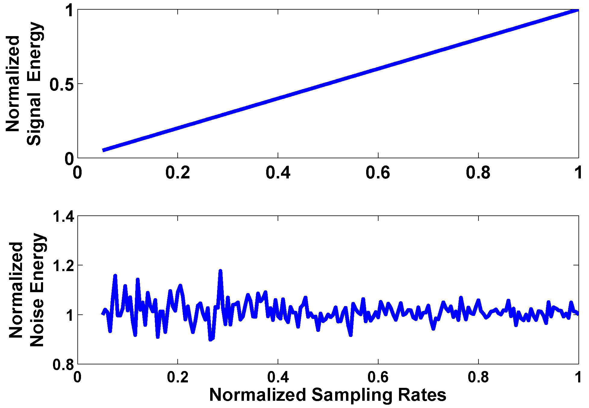
The detected signal energy level plays an important role in sub-Nyquist sampling. With sub-Nyquist sampling, we get lower signal SNR. Meanwhile, the energy detection results will be worse. What is shown in Figure 5 represents the relationship between the sampling rates and the detected signal energy.

The image appears to show that the detected signal energy is proportional to the sampling rates. However, the energy of noise changes randomly.

Inspired by Figure 5, we plot the sampling rates and related SNR of subsampled signal in Figure 6 to figure out how the sampling rates affect the signal SNR.

According to the figure, we can learn that the SNR of sub-sampled signal decreases along with the sampling rates. Furthermore, when the sampling rates decreases to half the Nyquist rate, the SNR decreases even more heavily. In other words, despite the fact that we can sense the spectrum with sub-Nyquist sampling rates, and we should use a higher sampling rate considering the correctness and effectiveness.

5.2. The Impact of Bandwidth Resolution

Assume that frequencies $f_1$ and $f_2$ are adjacent, let $\Delta f=|f_1-f_2|$. We define that bandwidth resolution is the minimum $\Delta f$ that we can distinguish from the detection. Bandwidth resolution is related to the observation time of FFT transformation. Long observation time gets better resolution. However, at the same time, the detection delay will increase. Otherwise, short observation time results in coarse resolution. For this section, we’ll investigate the influence on sub-Nyquist sensing of different bandwidth resolutionss.

The relationship between the bandwidth resolution and the detected energy is shown in Figure 7. We can easily figure out that both the energy of the signal and the noise is inversely proportional to the bandwidth resolution. If we increase the bandwidth resolution, the detected energy will decrease heavily.

5.3. The Impact of the SNR of the Original Signal

By original signal, we mean the signal before the ADC process here. The detection results are affected by the SNR of the original signal. Later, we’ll investigate the relationship between the original signal and the the signal SNR with sub-Nyquist rate.

We can learn from Figure 8 that, with sub-Nyquist sampling, we’ll get much lower SNR. Since sub-Nyquist sampling will worsen the SNR of the signal, we should carry out sub-Nyquist sensing under a relatively high SNR. The SNR of sub-Nyquist sampled signal is proportional to that of the original one and is much lower in value.

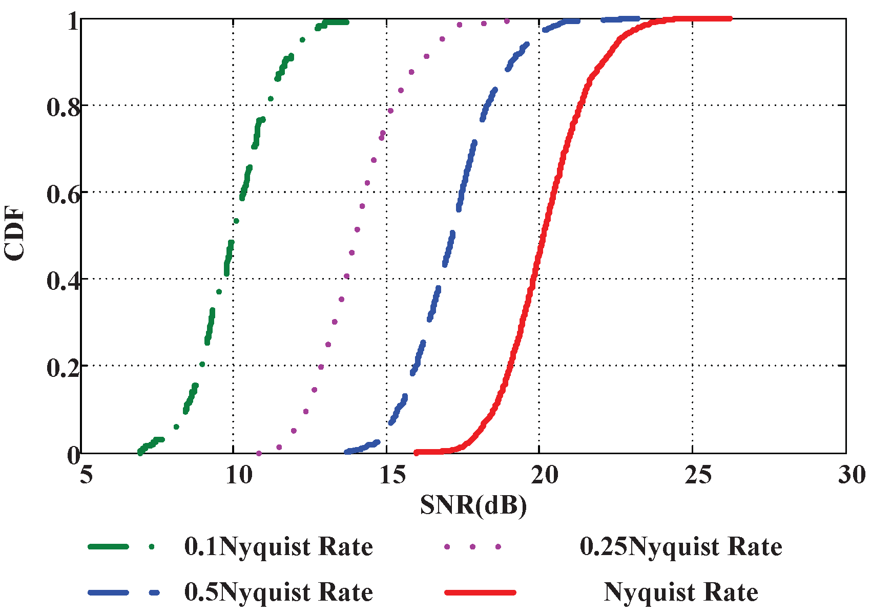
Figure 9 shows the Cumulative Distribution Function (CDF) of the SNR under different sampling rates. It is obvious that the lower the sampling rate is, the lower the SNR we get.

In short, the detection accuracy is mainly determined by the sampling rate and the signal SNR. We need to increase the sampling rate or improve the signal SNR if we want to get a better detection rate. Via these series of experiments, we can get a criteria on improvement of detection rate under different scenarios.

6. ASNSS: Adaptive Algorithm for SNSS

Despite the fact that ultra-wideband systems can correctly and effectively detect the spectrum occupancy, most of them have a fatal drawback. Wireless channel conditions are always dynamic, but their number of measurements are predetermined, so they can’t adjust to the circumstance changes. Due to the uncertainty of SNR and sparsity, most of the sub-Nyquist spectrum sensing systems suffer a great decrease of detection correctness. In consideration of the channel dynamic, we proposed adaptive sub-Nyquist spectrum sensing (ASNSS).

Currently, we consider two types of dynamics: (1) when the SNR of the PU’s signal becomes worse, a device may fail to determine the usage status accurately of a given channel. It is necessary to adopt a higher sampling rate and use a large FFT window to provide more processing gain, which can mitigate the effect of low SNR. (2) When more spectrum fragments are occupied, the percentage of uncertain channels will grow up when the bandwidth resolution is not changed.

6.1. Strength of PU’s Signal Changes

The detection probability of sub-Nyquist systems is greatly affected by the SNR. When the original SNR is reduced, the SNR condition of the sampled data also becomes worse. At this time, we need to adopt a higher sampling rate and larger FFT window to provide more processing gain.

• Detection. We set a threshold of the detected SNR of the signal, $SN{R}_{TH}$, when the SNR of the sampled data is lower than $SN{R}_{TH}$, i.e., $SN{R}_{DT}<SN{R}_{TH}$, the adaptive process is triggered.
• Adaptive policy. To improve the detected SNR, it is feasible to adopt a higher sampling rate and use more points in FFT.

Let $S_O$ be the current sampling rate, a factor $\beta$ is used to adjust the sampling rate. Usually, $\beta \in (0,1)$ is a function of the SNR, that is, $\beta =f(SN{R}_{sub},SN{R}_{Ny})$. Let $S_{max}$ be the highest sampling rate a device can support, we have

$$\begin{array}{cc}\hfill S_{New}& =\left\{\begin{array}{cc}{S}_O\ast (1+\beta ),\hfill & \hfill S_O\ast (1+\beta )<S_{max};\\ S_{max},\hfill & \hfill \mathrm{otherwise}.\end{array}\right.\hfill \end{array}$$

(15)

The adjustment is executed until the SNR returns back to a desired range or the sampling rate reaches the maximum one.

Similarly, when an increase of the SNR of sampled data is observed, the sampling rate can be returned to a low one. Let $S_{min}$ be a predefined minimum sampling rate, we have

$$\begin{array}{cc}\hfill S_{New}& =\left\{\begin{array}{cc}{S}_O\ast (1-\beta ),\hfill & \hfill S_O\ast (1-\beta )>S_{min};\\ S_{min},\hfill & \hfill \mathrm{otherwise}.\end{array}\right.\hfill \end{array}$$

(16)

6.2. Spectrum Occupancy Change

When more frequencies are utilized, to determine the spectrum usage, more devices are required to maintain the same bandwidth resolution.If the number of devices is fixed, we need to increase the bandwidth resolution in order to maintain the detection accuracy.

• Detection. We use the uncertain level to trigger the adaptive process. When the number of devices is too low, there will be some channels whose status cannot be determined uniquely.
• Adaptive policy. Let E be the number of the uncertain channels and $\theta$ be a predefined threshold, if $E>\theta$, which means that the status of a lot of channels cannot be determined. We set $\theta$ to be 0.1 in our simulations. At this time, it is necessary to increase the bandwidth resolution. Otherwise, the set of devices is not sufficient to monitor the spectrum. At this time, we try to decrease the resolution to obtain a more accurate view of the spectrum usage.

Note that, to increase the bandwidth resolution, one can either increase the sampling rate or decrease the FFT window size. Here, we prefer to increase the sampling rate first. Only when the sampling rate reaches the upper bound, we switch to decrease the FFT window size. In fact, after the increase of the bandwidth resolution, the detection accuracy is affected negatively if the FFT window is not increased accordingly. To maintain the same detection accuracy, the decrease of FFT window should be triggered cautiously.

6.3. ASNSS System

Based on the discussions above, we add a control unit that can change the number of sampling branches and corresponding sampling rates automatically to the SNSS system. The system is shown in Figure 10.

The control unit not only controls the number of sampling branches and its corresponding sampling rates, but also controls the window size of FFT transformation. The controller monitors the SNR of the signal and the occupancy of the frequency band in real time. Once it detects changes of SNR or occupancy, it will automatically adjust the sampling rates and FFT window size.

6.4. ASNSS Algorithm

The whole process of ASNSS is shown in Algorithm 2. First of all, the algorithm initializes all the variables, including signal bandwidth, spectrum occupancy and channel number.

During the sensing process, the algorithm monitors the SNR of the signal and the occupancy in real time. Once the SNR or the occupancy changes, the algorithm will adjust the sampling rates and the FFT window size immediately.

Algorithm 2: Adaptive Algorithm for SNSS

Data: Input: Signal Bandwidth $WB$, Spectrum Occupancy $\rho$, Channel Number N  Data: Output: Spectrum Occupancy Vector $\mathbf{F}$   1 ${\mathbf{F}}_{{\mathbf{s}}_{max}}\leftarrow (f_{1_{max}},f_{2_{max}},f_{3_{max}},\cdots ,f_{{\gamma }_{max}})$;   2 Set the maximum sampling rate of each device;   3 ${\mathbf{F}}_{{\mathbf{s}}_{min}}\leftarrow (f_{1_{min}},f_{2_{min}},f_{3_{min}},\cdots ,f_{{\gamma }_{min}})$;   4 Set the minimum sampling rate of each device;   5 $\mathbf{FFTWINDOW}\leftarrow (FF{T}_1,FF{T}_2,FF{T}_3,\cdots ,FF{T}_{\gamma })$;   6 Initialize the window size of FFT transformation;   7 $\alpha \leftarrow f(SN{R}_{Sub},SN{R}_{Ny})$;   8 β is the sampling rate adjustment factor, $\alpha \in (0,1)$;   9 INITIALIZE $\beta$; 10 INITIALIZE $Occupanc{y}_{low},Occupanc{y}_{high}$; 11 $\mathbf{F}\leftarrow (0,0,0,\cdots ,0)$; 12 Initialize Spectrum Occupancy Vector; 13 $\gamma \leftarrow \eta \rho +\theta$; 14 Initialize the number of sampling Branches, their value are defined in Equation (13); 15 ${\mathbf{F}}_{\mathbf{s}}\leftarrow (f_1,f_2,f_3,\cdots ,f_{\gamma })$; 16 Initialize sampling rates; 17 INITIALIZE $SN{R}_{low}$, $SN{R}_{high}$; 18 When $SNR<SN{R}_{low}$, increase the sampling rates; or when $SNR>SN{R}_{high}$ decrease the sampling rates; 19 $Occupancy\leftarrow \rho$;

7. Performance Evaluation

In this part, we’ll evaluate the performance of our algorithm. The performance of the algorithm is evaluated by simulations. We make all the simulations on MATLAB R2014b software platform. We set the signal bandwidth to be 1 G, and the maximum sampling rate of each equipment is 100 MHz (the same as USRP N210). Channels are abstracted to a set of sequences. We set the channel to be “1” when the channel is occupied. Otherwise, we set the channel to be “0”.

7.1. SNSS Performance

First of all, we evaluate the performance of SNSS under different occupancies. As we all know, the occupancy is directly related to the detection accuracy. Figure 11 shows the detection rate of SNSS under different occupancies. From the figure, we can learn that, under low SNR, the detection rate is severely affected by the occupancy. When the occupancy increases, the detection rate decreases quickly, while, under high SNR, there is little difference in performance under different occupancies. We can get a high accuracy under each occupancy from $5\%$ to $40\%$.

The detection rate under different SNRs is shown in Figure 12. Obviously, the higher the SNR, the higher the detection rate. In consideration of the spectrum occupancy, in reality (about 7%), our algorithm can get an average accuracy of 99% when SNR is 15 dB. When the SNR is 10 dB, SNSS can still reach an accuracy of 85%.

Figure 13 and Figure 14 show the detection rate with different bandwidth resolutions under different occupancies and different SNRs. As the figure shows, both under different occupancies and under different SNRs, we can get a higher accuracy with larger bandwidth resolution. That is to say, when we encounter worse accuracy, we can properly lower the bandwidth resolution. Though we may get a coarse result, but it is accurate.

7.2. ASNSS Performance

The probability of detection with time-varying SNR is shown in Figure 15. As we can learn from the figure, the SNR value has a deep influence on the detection accuracy. As long as the SNR value is high, we’ll get a high detection accuracy even if the sampling rate is relatively low. However, when the SNR value becomes lower, the performance decreases significantly at a low sampling rate. In addition, when the sampling rate is high, the detection accuracy is high but at the cost of more energy consumption and higher computation complexity. By use of an adaptive policy, one can maintain the same high accuracy by using a reasonable sampling rate at different SNRs conditions.

The detection accuracies under different spectrum utilization ratios are shown in Figure 16. With low utilization ratio, we can get a fine-grained resolution of the spectrum usage. However, with a high utilization ratio, we can hardly maintain the accuracy with the same granularity. We need to add more devices or just adopt the resolution to a coarse one to get a high accuracy. By the adaptive policy, one can automatically provide an accurate usage view at low utilization ratio and a coarse-grained usage view with the same high accuracy.

8. Conclusions and Future Work

Ultra-wideband spectrum sensing is quite important to the future high speed cognitive communication. In terms of the limit to manufacture high speed ADCs, sub-Nyquist sampling methods show a great potential to future ultra-wideband spectrum sensing. We first propose a sub-Nyquist spectrum sensing algorithm SNSS which can simplify the system architecture and reduce the computation amount. When the signal SNR is 15 dB, the average detection rate of SNSS reaches 99% under the occupancy of 7%. Even if the SNR is as low as 10 dB, SNSS can still get an accuracy of 85%. Then, we conduct an extensive study to investigate the influence on the performance of sub-Nyquist sensing of several factors such as sampling rate, bandwidth resolution and the signal SNR. Afterwards, an adaptive policy is discussed to determine the optimal parameters to track the PU’s behaviors.

For future work, we plan to study the optimal setting where the spectrum occupation ratio is high.

References

- Cisco. Cisco Visual Networking Index: Global Mobile Data Traffic Forecast Update, 2017–2022; Technical Report; Cisco: San Jose, CA, USA, 2018. [Google Scholar]
- Koenig, S.; Lopez-Diaz, D.; Antes, J.; Boes, F.; Henneberger, R.; Leuther, A.; Tessmann, A.; Schmogrow, R.; Hillerkuss, D.; Palmer, R.; et al. Wireless sub-THz communication system with high data rate. Nat. Photonics 2013, 7, 977–981. [Google Scholar] [CrossRef]
- McHenry, M. NSF Spectrum Occupancy Measurements Project Summary; Shared Spectrum Company: Vienna, VA, USA, 2005. [Google Scholar]
- Mitola, J. Cognitive Radio—An Integrated Agent Architecture for Software Defined Radio. Ph.D. Thesis, Royal Institute of Technology, Stockholm, Sweden, 2000. [Google Scholar]
- Cavalcante, A.M.; Almeida, E.; Vieira, R.D.; Chaves, F.; Paiva, R.C.; Abinader, F.; Choudhury, S.; Tuomaala, E.; Doppler, K. Performance evaluation of LTE and Wi-Fi coexistence in unlicensed bands. In Proceedings of the 2013 IEEE 77th Vehicular Technology Conference (VTC Spring), Dresden, Germany, 2–5 June 2013; pp. 1–6. [Google Scholar]
- Tandra, R.; Sahai, A. Fundamental limits on detection in low SNR under noise uncertainty. In Proceedings of the 2005 International Conference on Wireless Networks, Communications and Mobile Computing, Maui, HI, USA, 13–16 June 2005; Volume 1, pp. 464–469. [Google Scholar] [CrossRef]
- Urkowitz, H. Energy detection of unknown deterministic signals. Proc. IEEE 1967, 55, 523–531. [Google Scholar] [CrossRef]
- Shankar, N.; Cordeiro, C.; Challapali, K. Spectrum agile radios: Utilization and sensing architectures. In Proceedings of the First IEEE International Symposium on New Frontiers in Dynamic Spectrum Access Networks, DySPAN 2005, Baltimore, MD, USA, 8–11 November 2005; pp. 160–169. [Google Scholar] [CrossRef]
- Xia, X.G. On estimation of multiple frequencies in undersampled complex valued waveforms. IEEE Trans. Signal Proc. 1999, 47, 3417–3419. [Google Scholar] [CrossRef]
- Hassanieh, H.; Shi, L.; Abari, O.; Hamed, E.; Katabi, D. GHz-Wide Sensing and Decoding Using the Sparse Fourier Transform. In Proceedings of the 33rd Annual IEEE International Conference on Computer Communications (INFOCOM’14), Toronto, ON, Canada, 27 April–2 May 2014. [Google Scholar]
- Quan, Z.; Cui, S.; Sayed, A.H.; Poor, H.V. Optimal multiband joint detection for spectrum sensing in cognitive radio networks. IEEE Trans. Signal Process. 2009, 57, 1128–1140. [Google Scholar] [CrossRef]
- Tian, Z.; Giannakis, G.B. A wavelet approach to wideband spectrum sensing for cognitive radios. In Proceedings of the 1st International Conference on Cognitive Radio Oriented Wireless Networks and Communications, Mykonos Island, Greece, 8–10 June 2006; pp. 1–5. [Google Scholar]
- Yoon, S.; Li, L.E.; Liew, S.C.; Choudhury, R.R.; Rhee, I.; Tan, K. QuickSense: Fast and energy-efficient channel sensing for dynamic spectrum access networks. In IEEE INFOCOM; Institute of Electrical and Electronics Engineers Inc.: Turin, Italy, 2013; pp. 2247–2255. [Google Scholar]
- Tian, Z.; Giannakis, G.B. Compressed sensing for wideband cognitive radios. In ICASSP, IEEE International Conference on Acoustics, Speech and Signal Processing; Institute of Electrical and Electronics Engineers Inc.: Honolulu, HI, USA, 2007; Volume 4, pp. IV1357–IV1360. [Google Scholar]
- Axell, E.; Leus, G.; Larsson, E.G.; Poor, H.V. Spectrum sensing for cognitive radio: State-of-the-art and recent advances. IEEE Signal Process. Mag. 2012, 29, 101–116. [Google Scholar] [CrossRef]
- Ding, C. Chinese Remainder Theorem; World Scientific: Singapore, 1996. [Google Scholar]
Figure 1.
Illustration of aliasing.
Figure 2.
Illustration of the basic idea of sub-Nyquist sensing. (a) Sampling result with ; (b) Sampling result with .
Figure 3.
System view of SNSS.
Figure 4.
Illustration of the work process of sub-Nyquist wideband spectrum sensing.
Figure 5.
The relationship between the sampling rate and the detected signal energy. The sampling rates are normalized with respect to the Nyquist rate.
Figure 6.
The signal SNR for different sampling rates. The vertical dash line stands for the Nyquist rate and the horizonal one represents the SNR detected under Nyquist sampling rate.
Figure 7.
The impact of bandwidth resolution. The x-axis stands for the actual bandwidth resolution.
Figure 8.
The signal SNR before and after sub-Nyquist sampling.
Figure 9.
The CDF of SNR under different sampling rates.
Figure 10.
The ASNSS system.
Figure 11.
Detection rate under different occupancies.
Figure 12.
Detection rate under different SNRs.
Figure 13.
Detection rate under different occupancies with different bandwidth resolutions.
Figure 14.
Detection rate under different SNRs with different bandwidth resolutions.
Figure 15.
Detection probability under different SNRs.
Figure 16.
Detection accuracy under different spectrum utilization levels.
© 2019 by the authors. Licensee MDPI, Basel, Switzerland. This article is an open access article distributed under the terms and conditions of the Creative Commons Attribution (CC BY) license (http://creativecommons.org/licenses/by/4.0/).
Share and Cite
MDPI and ACS Style
Lu, Y.; Lv, S.; Wang, X. Adaptive Sub-Nyquist Spectrum Sensing for Ultra-Wideband Communication Systems. Symmetry 2019, 11, 342. https://doi.org/10.3390/sym11030342
AMA Style
Lu Y, Lv S, Wang X. Adaptive Sub-Nyquist Spectrum Sensing for Ultra-Wideband Communication Systems. Symmetry. 2019; 11(3):342. https://doi.org/10.3390/sym11030342
Chicago/Turabian StyleLu, Yong, Shaohe Lv, and Xiaodong Wang. 2019. "Adaptive Sub-Nyquist Spectrum Sensing for Ultra-Wideband Communication Systems" Symmetry 11, no. 3: 342. https://doi.org/10.3390/sym11030342
Note that from the first issue of 2016, this journal uses article numbers instead of page numbers. See further details here.