Hysteretic Loops in Correlation with the Maximum Dissipated Energy, for Linear Dynamic Systems

Research Institute for Construction Equipment and Technology—ICECON S.A., 021652 București, Romania
Symmetry 2019, 11(3), 315; https://doi.org/10.3390/sym11030315
Submission received: 17 December 2018
/
Revised: 21 February 2019
/
Accepted: 21 February 2019
/
Published: 2 March 2019
Abstract
:This paper presents the outcomes of the theoretical and experimental research carried out on a real model at natural scale using Voigt–Kelvin linear viscoelastic type m, c, and k models excited by a harmonic force F(t) = F0 sinωt, where F0 is the amplitude of the harmonic force and ω is the excitation angular frequency. The linear viscous-elastic rheological system (m, c, k) is characterized by the fact that the c linear viscous damping—and, consequently, the fraction of the critical damping ζ—may be changed so that the dissipated energy can reach maximum values. The optimization condition between the maximum dissipated energy and the amortization modifies the structure of the relation F = F(x), which describes the elliptical hysteresis loop F–x in the sense that it has its large axis making an angle less than 90° with respect to the x-axis in ante-resonance, and an angle greater than 90° in post-resonance for . The elliptical Q–x hysteretic loops are tilted with their large axis only at angles below 90°. It can be noticed that the equality between the arias of the hysteretic loop, in the two representations systems Q–x and F–x, is verified, both being equal with the maximum dissipated energy .
1. Introduction
For the vibration-driven technological processes with excitation harmonic forces, Voigt–Kelvin linear rheological models are adopted with the discretionary variation of the amortization or of the fraction of the critical amortization .
The functional optimization of the vibration-driven processes consists of reaching a maximum dissipated energy for in direct correlation with the area of the elliptical hysteretic loop. By locating suitable transducers on the physical system, the elliptical hysteretic loops can be determined in such a manner that allows the assessment of their areas, respectively the maximum dissipated energy for a dynamic system may be assessed with rigidity k and amplitude A of the instantaneous displacement , where φ is the phase angle.
Depending on the optimization requirement, in order to achieve a maximum dissipation, i.e., , can be determined the pairs of values for which are established the calculus relations of the significant parameters. Thus, the functional relations were established for A = A(ω), amplitude, the dissipated energy, the viscoelastic force , and the excitation force F = F(x). The correlations between the maximum dissipated energy and the areas of the elliptical hysteretic loops are reflected in the graphical representations for the case of operation in ante-resonance at and respectively for the case of post-resonance at [1,2,3].
Experimental research carried out so far has mainly highlighted the positioning of hysteretic loops as an ante-resonance regime for testing elastomeric devices. The results highlighted in this field, both linearly and nonlinearly, are presented in papers published by various researchers from Italy, France, USA, and Romania [4,5,6,7,8,9,10]. Interpretation of experimental results and behavioral modeling of elastomeric device behavior are addressed in published reference works [11,12,13,14,15,16,17,18]. To highlight the post-resonance regime, interesting and useful research is contained in some published papers cited in the literature [19,20,21,22,23].
In this paper are highlighted the hysteretic loops families of the elastomeric devices that were designed, manufactured and tested, for a viaduct on the “Transilvania” Motorway, in Romania. Thus, based on dynamic testing devices and realized within ICECON Bucharest (Romania), there were determined the characeristic shapes of the hysteretic loops for the three dynamic regimmes, namely: ante-resonance, resonance, and post-resonance.
The characteristic function for dissipated energy was also established, highlighting its modification in relation to the fraction of critical damping ζ as a system parameter.
The novelty of the approach consists of the fact that for the elastomeric isolator system/device are highlighted the dissipative characteristics, the hysteretic loop orientation, as well as the dissipated energy variation depending on the parameter ζ, which can take different values in relation to mass m, elasticity k, and linear dissipation c. The graphical representation of the hysteretic loop in accordance with the dissipated energy allowed a clearer, more operational and efficient highlighting of the dynamic behavior during the tests, with meaningful and eloquent conclusions.
2. Parameter Analysis
The dynamic linear models m, c, and k, produced by the harmonic force F(t) = F0 sinωt and with the reaction force Q(t) in the liniar viscoelastic system, c, k, is presented in Figure 1.
The movement equation at the dynamic balance is
The solution of Equation (1) is
where A is the amplitude of the instantaneous displacement x = x(t), is the phase shift between the instantaneous displacement x(t) and the excitation force F(t).
It is introduced the notation: , where , so that the variable to be used as excitation relative pulsation.
2.1. Amplitude of Displacement
An amplitude of the instantaneous displacement x = x(t) may be expressed by the A(ω) or A(Ω) relation, as follows:
or
2.2. De-Phasing between Force and Displacement
The de-phasing φ between the excitation force F = F(t) and the instantaneous displacement x = x(t) may be calculated as follows:
or
2.3. Dissipated Energy
The dissipated energy Wd may be expressed according to and as follows:
where .
From the condition of maximum Wd, which is , it emerges that , so that the maximum dissipated energy becomes
It can be noticed that for certain values of it correspond the values of for which the dissipated energy is at maximum. The representation of , so that the variation domain of to be included , leads to a curve with a maximum point, having the coordinates at . For the discrete values of , a family of parametrical curves of can be obtained.
2.4. Equation of the F–x Elliptic Hysteretic Loop
Phase is eliminated between x = x(t) and F = F(t) as follows:
where , , resulting
If we note the dimensionless sizes and , then relation (10) becomes
From of equation (11) emerges as
where and .
By replacing , , , and in relation (12), the expression of force F emerges according to pulsation , rigidity k, and amortization c as follows:
or in terms of and measures we have
For the condition that the dissipated energy to be maximum, at .
- (a)
- For the ante-resonance regime at , obtainingor
- (b)
- For the post-resonance regime at the following is obtained:orwhereor
2.5. Equation of the Hysteretic Loop Q–x
The instantaneous viscous-elastic force may be expressed from the dynamic equilibrium equation. Thus, it can be expressed or
from where Q(t) emerges as , or in relation with x = x(t), it is obtained
In Equation (22) we insert the expression of force from (13) and have
and in relation with Equation (23) becomes
It is found that the family of ellipses according to Equation (24) is characterized by the fact that all ellipses have their major axis in the quadrant (0, π/2) with positive angular coefficient for any value , where is the angle between the ellipse axis and the Ox axis [24].
3. Elliptic Hysteretic Loops for the Ante-Resonance Regime ()
For a dynamic system where m = 104 kg, k = 2⋅107 N/m at the relative pulses Ω1 = 0.8 with ; Ω2 = 0.6 with ; and Ω3 = 0.5 with , the representation of the elliptical hysteretic loops Q–x and F–x, according to the graph of function Wd = W(ζ), as shown in Figure 2, Figure 3 and Figure 4. In each figure functions F(x) and Q(x) are represented based on Equations (16) and (24), respectively, corresponding to the representation of function Wdmax = W(ζ), given by Equation (8). Thus, it is found that for the maximum value of the dissipated energy Wdmax according to and , i = 1, 2, 3, the areas of the ellipses F–x and Q–x are maximum and equal [25,26,27,28,29]
We specify the fact that the fraction of the critical amortization , in this case for Wd max, may be defined as follows:
and taking into account Equations (8) and (20), we have
It can be observed that only at a resonance, when , it results .
4. Elliptic Hysteretic Loops for the Post-Resonance Regime ()
5. Conclusions
The dynamic linear system m, c, and k excited by a harmonic perturbatory force is assessed dynamic regimes of ante-resonance and and post-resonance for values of the viscous dumping , for which the dissipated energy is maximum: .
- (a)
- For this, there are established the functional relations of the perturbatory force F = F(x) in relation with the instantaneous displacement x = x(t), of the viscoelastic force Q = Q(t) in relation with x = x(t), of the viscoelastic force Q = Q(x) in relation with x = x(t), and of the dissipated energy in relation with the variation of the viscous dumping , namely Wd = W(ζ);
- (b)
- In this context, based on the graphical representations, it was possible to emphasize the fact that the ellipses F–x are rotating in relation to the origin of the axis system, according to the dynamic regime or . The axis of the ellipse F–x rotation is caused by the inertial effect that is produced by the presence of the factor in the expression of the function F = F(x);
- (c)
- The representation of the function Q = Q(x) highlights the that it constantly maintains an angle of inclination of the ellipse Q–x, axis, with a positive slope;
- (d)
- It can be noticed that the areas of the hysteretic loops F–x and Q–x are equal between them and equal with the maximum value of the dissipated energy Wmax () for .
- (e)
- The effective critical dumping depends both on the value of as well as on the relative pulsation , for ante-resonance or , for post-resonance. In the case of the resonance regime, for , then is a sole situation that enables the assessment of the fraction from the optimal critical amortization .
The concordant graphical representations eloquently demonstrated the fact that for the dynamic regimes defined by the relative pulsation , the dissipative effects of the linear viscous-elastic systems may be analyzed, in experimental conditions defined by specific requirements.
The obtained results are based on the experimental tests performed on dynamic testing systems using real manufactured products. The tests were carried out in laboratories specialized in the testing of anti-vibration and anti-seismic devices, and the devices, belonging to recognized laboratories or manufacturing companies such as SISMALAB (Italy), EUCENTRE (Italy), DIS (Reno, USA), ALGA (Italy), and ICECON (Romania).
Based on the researches and the results presented in this paper, were designed and manufactured the elastomeric anti-seismic devices used for a viaduct with a length of 200 m, on the “Transilvania” Motorway, constructed by the Bechtel company (USA), in Romania.
The experimental tests performed in order to determine the hysterical loop families were conducted within the ICECON Romanian Research Institute for Construction Equipment and Technology – ICECON, using both anti-vibration and anti-seismic devices.
The assessment system using specialized tests was based on the Romanian Patent No. 80484/1982 “Stand for the measurement of the mechanical characteristics of rubber”, whose owner is the author of this paper.
Funding
This research received no external funding.
Conflicts of Interest
The authors declare no conflict of interest.
References
- Dobrescu, C. The Rheological Behaviour of Stabilized Bioactive Soils During the Vibration Compaction Process for Road Structures. In Proceedings of the 22th International Congress on Sound and Vibration, Florence, Italy, 12–16 July 2015. [Google Scholar]
- Mitu, A.M.; Sireteanu, T.; Ghita, G. Passive and semi-active bracing systems for seismic protection: A comparative study. Rom. J. Acoust. Vib. 2015, 12, 49–56. [Google Scholar]
- Sireteanu, T. Smart suspension systems. Rom. J. Acoust. Vib. 2016, 13, 2. [Google Scholar]
- Conveney, V.V.; Johnson, D.E.; Kulak, R.F. Modelling the Free Oscillation of Building Suported on High Damping Rubber Isolators. In Proceedings of the Seismic Engineering 2000, The 2000 ASME Pressure Vessels and Piping Conference, Seattle, WA, USA, 23–27 July 2000; Volume 1. [Google Scholar]
- Lin, S.B. Theoretical and Experimental Study of High Damping Rubber Bearing and Lead Extrusion Damper. Master’s Thesis, Feng Chia University, Taichung, Taiwan, 2000. [Google Scholar]
- Chen, B.J.; Lin, S.B.; Tsai, C.S. Theoretical and Experimental Study of High Damping Rubber Bearings. In Proceedings of the Seismic Engineering 2001, The 2000 ASME Pressure Vessels and Piping Conference, Seattle, WA, USA, 23–27 July; Volume 2.
- Dolce, M.; Ponzo, F.C.; Di Cesare, A.; Arlego, G. Progetto di Edifici con Isolamento Sismico; IUSS Press: Pavia, Italy, 2010. [Google Scholar]
- Marioni, A. Sisitemi di Isplamento Sismico Innovetivi Prodotti dalla Societa ALGA. In Moderni Sistemi e Tecnologie Antisismici. Una Guida per il Progettista; 21mo Secolo: Milano, Italy, 2008. [Google Scholar]
- Bratu, P. Vibration Transmissivity in Mechanical Systems with Rubber Elements Using Viscoelastic Models. In Proceedings of the 5th European Rheology Conference, Ljubljana, Slovenia, 6–11 September 1998. [Google Scholar]
- Delfosse, C.G. Étude des vibrations linéaires d’un systeme mecanique complexe par méthode des mates normaux. Ann. l’ITBTP 1976, 336, 122–136. [Google Scholar]
- Giacchetti, R. Fondamente di Dinamica delle Strutture e di Ingineria Sismica; EPC Libri: Roma, Italy, 2004. [Google Scholar]
- Bratu, P. Analyze Insulator Rubber Elements Subjected to Actual Dynamic Regime. In Proceedings of the 9th International Congress Sound and Vibration, Orlando, FL, USA, 8–11 July 2002. [Google Scholar]
- Bratu, P. Experimental evaluation of the antivibrating damping capacity in case of elastomers used for tram railway supportins. Mater. Plast. 2009, 46, 127–130. [Google Scholar]
- Bratu, P. Rheological model of the neopren elements used for base isolation against seismic actions. Mater. Plast. 2009, 46, 288–294. [Google Scholar]
- Jennings, P. Equivalent viscous damping for yelding structures. J. Eng. Mech. Division 1968, 94, 103–116. [Google Scholar]
- Rao, M. Mechanical Vibrations; Addison-Wesley Pub. Co.: Boston, MA, USA, 2011. [Google Scholar]
- Sireteanu, T.; Giuclea, M.; Mitu, A.M. An analitical approach for approximation of exxperimental hysteretic by Bouc.-Wen model. Procc. Rom. Acad. Ser. A 2009, 10, 4354. [Google Scholar]
- Sireteanu, T.; Giuclea, M.; Mitu, A.M. Identification of an extended Bouc.-Wen model with application to seismic protection through hysteretic devices. Comput. Mech. 2010, 45, 5. [Google Scholar] [CrossRef]
- Le Tallec, P. Introduction à la Dynamique des Structures; Cépaduès: Toulouse, France, 2000. [Google Scholar]
- Trigili, G. Introduzione alla Dinamica delle Strutture e Spettri di Progeto; Laccorio: Palermo, Italy, 2010. [Google Scholar]
- Dolce, M.; Mortelli, A.; Panza, G. Proteggersi dal Terremoto; 21/mo Secolo: Milano, Italy, 2004. [Google Scholar]
- Mortelli, A.; Sannino, U.; Parducci, A.; Braga, F. Moderni Sistemi e Tecnologie Antisismici Una Guida per il Progettista; 21mo Secolo: Milano, Italy, 2008. [Google Scholar]
- Radeș, M. Mechanical Vibrationes; Ed. Printech: București, Romania, 2006. [Google Scholar]
- Johnson, E.A.; Ramallo, J.C.; Spencer, B.F., Jr.; Sain, M.K. Intelligent Base Isolation Systems. In Proceedings of the 2nd World Conference on Structural Control, Kyoto, Japan, 28 June–1 July 1998. [Google Scholar]
- Wang, Y.-P. Fundamentals of Seismic Base Isolation. In International Training Programs for Seismic Design of Building Structures; National Certer of Research on Earthquake Engineering: Taipei, Taiwan, 2016. [Google Scholar]
- Stanescu, N.D. Vibrations of a shell with clearances, neo-Hookean stiffness, and harmonic excitations. Rom. J. Acoust. Vib. 2016, 13, 104–111. [Google Scholar]
- Vasile, O. Active vibration control for viscoelastic damping systems under the action of inertial forces. Rom. J. Acoust. Vib. 2017, 14, 54–58. [Google Scholar]
- Inman, D. Vibration with Control; John Wiley & Sons Ltd.: London, UK, 2007. [Google Scholar]
- Najari, S. Identification par Analyse Harmonique des Structures en Géniè Civil; INSA: Toulouse, France, 1981. [Google Scholar]
Figure 1.
Linear dynamic model m, c, and k.
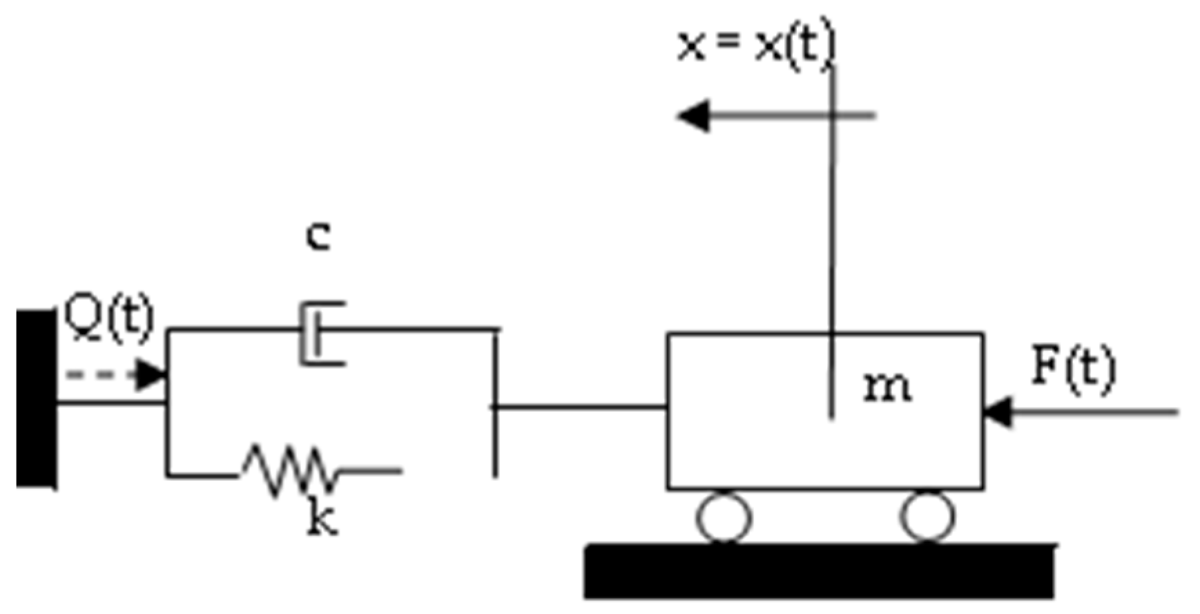
Figure 2.
Variation curves in ante-resonance for W1max at Ω1 = 0.8 and ζ1 = 0.225. (a) Variation of W1 according to ζ. (b) Elliptic hysteretic loop F1–x. (c) Elliptic hysteretic loop Q1–x. x = [−0.08701 ÷ +0.08701].
Figure 2.
Variation curves in ante-resonance for W1max at Ω1 = 0.8 and ζ1 = 0.225. (a) Variation of W1 according to ζ. (b) Elliptic hysteretic loop F1–x. (c) Elliptic hysteretic loop Q1–x. x = [−0.08701 ÷ +0.08701].
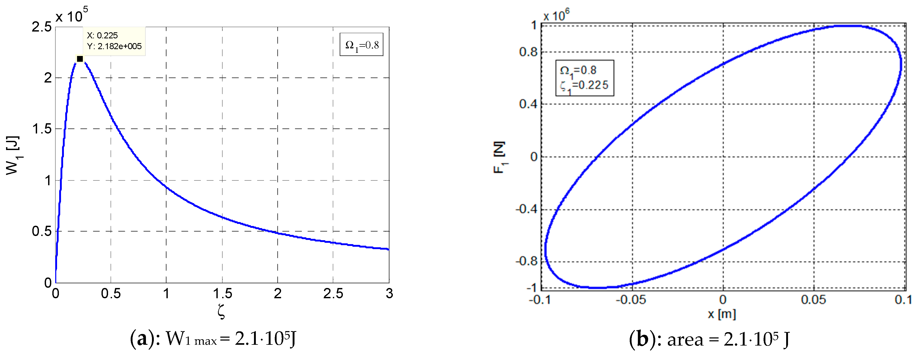
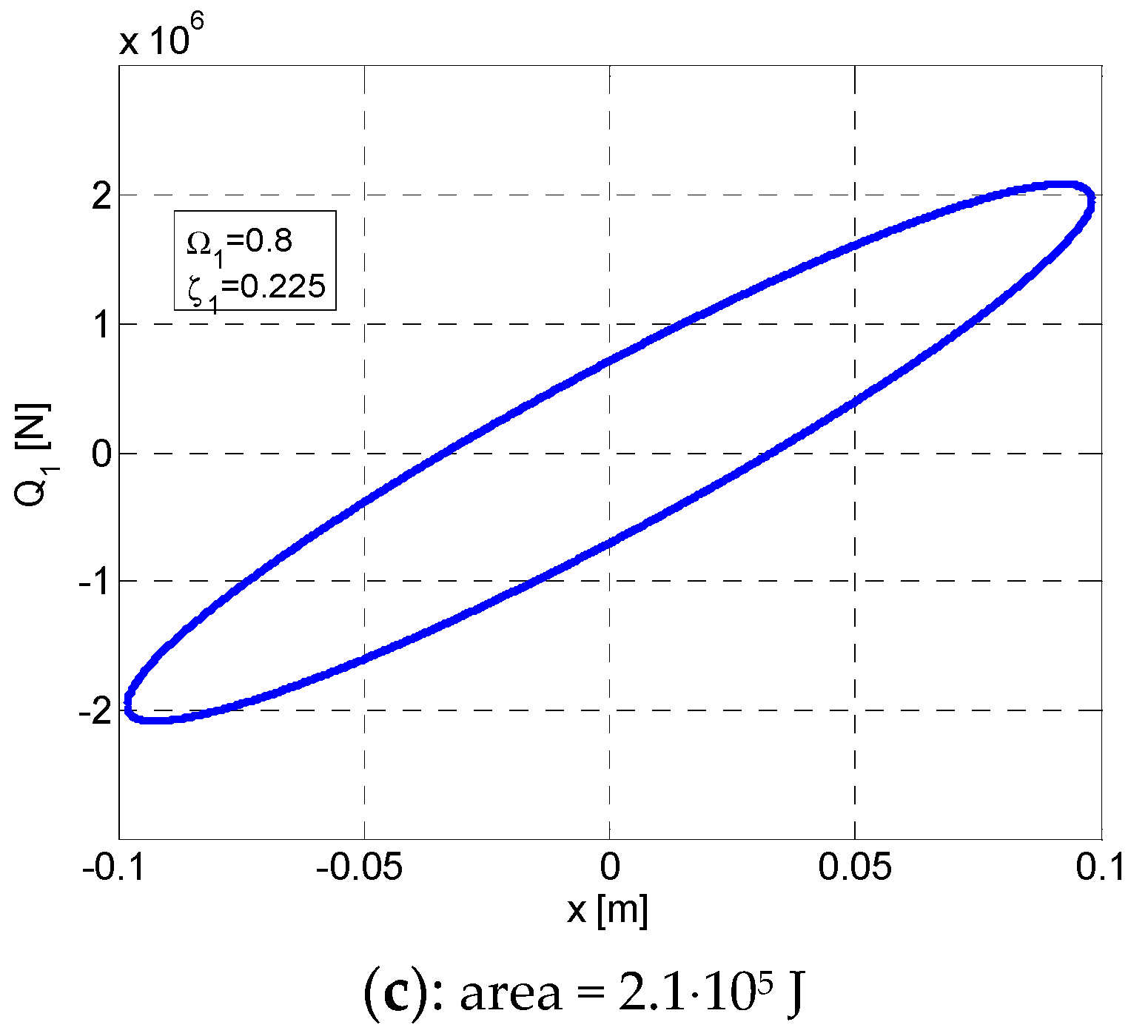
Figure 3.
Variation curves in ante-resonance for W2max at Ω2 = 0.6 and ζ2 = 0.53. (a) Variation of W2 according to ζ. (b) Elliptic hysteretic loop F2–x. (c) Elliptic hysteretic loop Q2–x. x = [−0.05542 ÷ +0.05542].
Figure 3.
Variation curves in ante-resonance for W2max at Ω2 = 0.6 and ζ2 = 0.53. (a) Variation of W2 according to ζ. (b) Elliptic hysteretic loop F2–x. (c) Elliptic hysteretic loop Q2–x. x = [−0.05542 ÷ +0.05542].

Figure 4.
Variation curves in ante-resonance for W3max at Ω3 = 0.5 and ζ3 = 0.75. (a) Variation of W3 according to ζ. (b) Elliptic hysteretic loop F3–x. (c) Elliptic hysteretic loop Q3–x. x = [−0.04715 ÷ +0.04715].
Figure 4.
Variation curves in ante-resonance for W3max at Ω3 = 0.5 and ζ3 = 0.75. (a) Variation of W3 according to ζ. (b) Elliptic hysteretic loop F3–x. (c) Elliptic hysteretic loop Q3–x. x = [−0.04715 ÷ +0.04715].
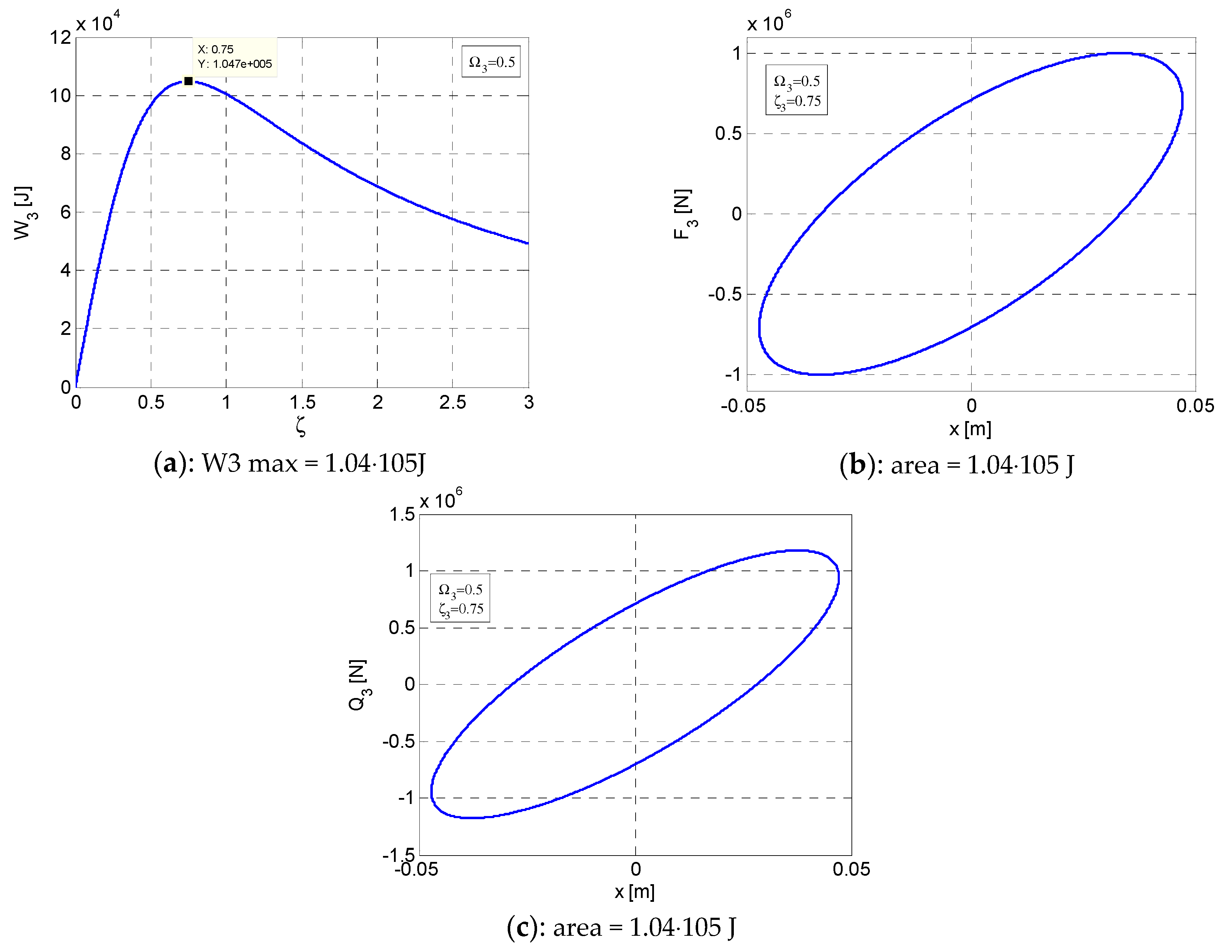
Figure 5.
Families of curves in ante-resonance for W1max, W2max, and W3max. (a) Families of curves W according to the current variable ζ and the discreet variable Ω. (b) The family of elliptical hysteretic loops F–x according to the current variable x and the pair of discreet variables Ω, ζ. (c) The family of elliptical hysteretic loops Q–x according to the current variable x and the pair of discreet variables Ω, ζ.
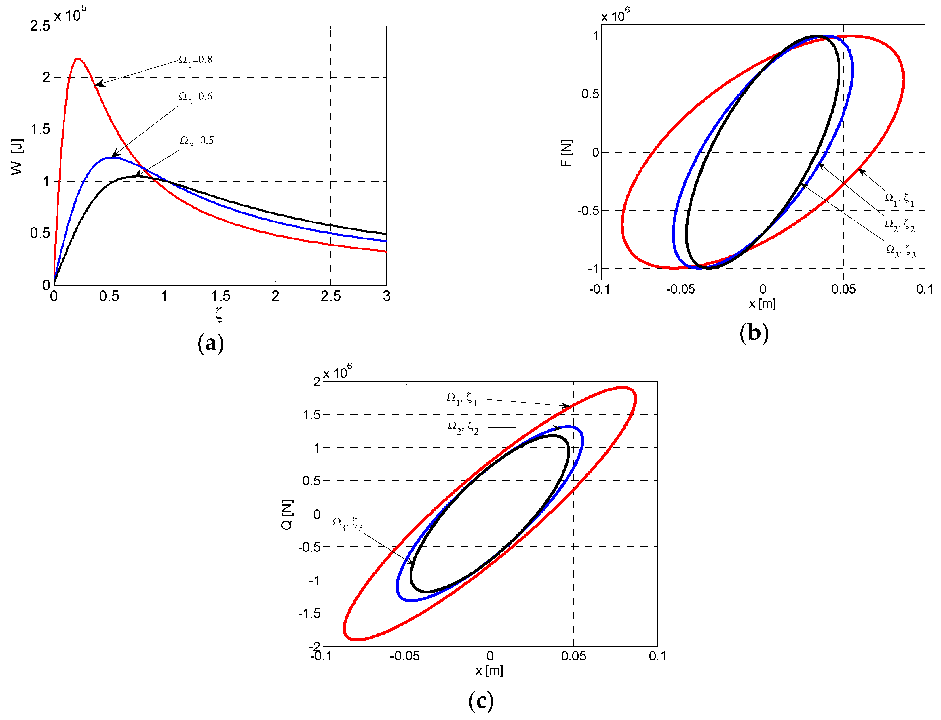
Figure 6.
Variation curves in post-resonance for W4max at Ω4 = 1.31 and ζ4 = 0.28. (a) Variation of W4 according to ζ. (b) Elliptic hysteretic loop F4–x. (c) Elliptic hysteretic loop Q4–x. x = [−0.04878 ÷ +0.04878].
Figure 6.
Variation curves in post-resonance for W4max at Ω4 = 1.31 and ζ4 = 0.28. (a) Variation of W4 according to ζ. (b) Elliptic hysteretic loop F4–x. (c) Elliptic hysteretic loop Q4–x. x = [−0.04878 ÷ +0.04878].
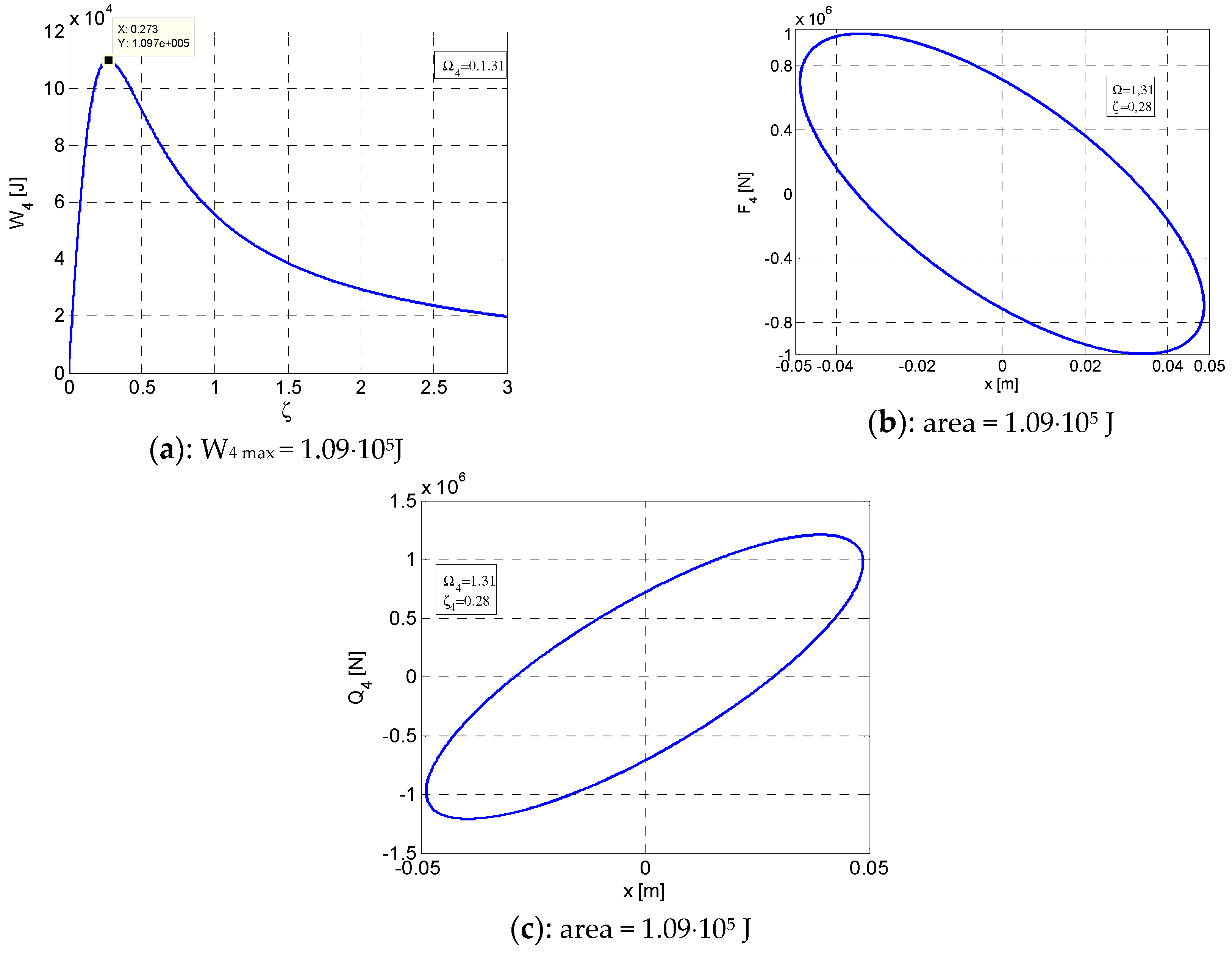
Figure 7.
Variation curves in post-resonance for W5max at Ω5 = 1.66 and ζ5 = 0.53. (a) Variation of W5 according to ζ. (b) Elliptic hysteretic loop F5–x. (c) Elliptic hysteretic loop Q5–x. x = [−0.02012 ÷ +0.02012].
Figure 7.
Variation curves in post-resonance for W5max at Ω5 = 1.66 and ζ5 = 0.53. (a) Variation of W5 according to ζ. (b) Elliptic hysteretic loop F5–x. (c) Elliptic hysteretic loop Q5–x. x = [−0.02012 ÷ +0.02012].
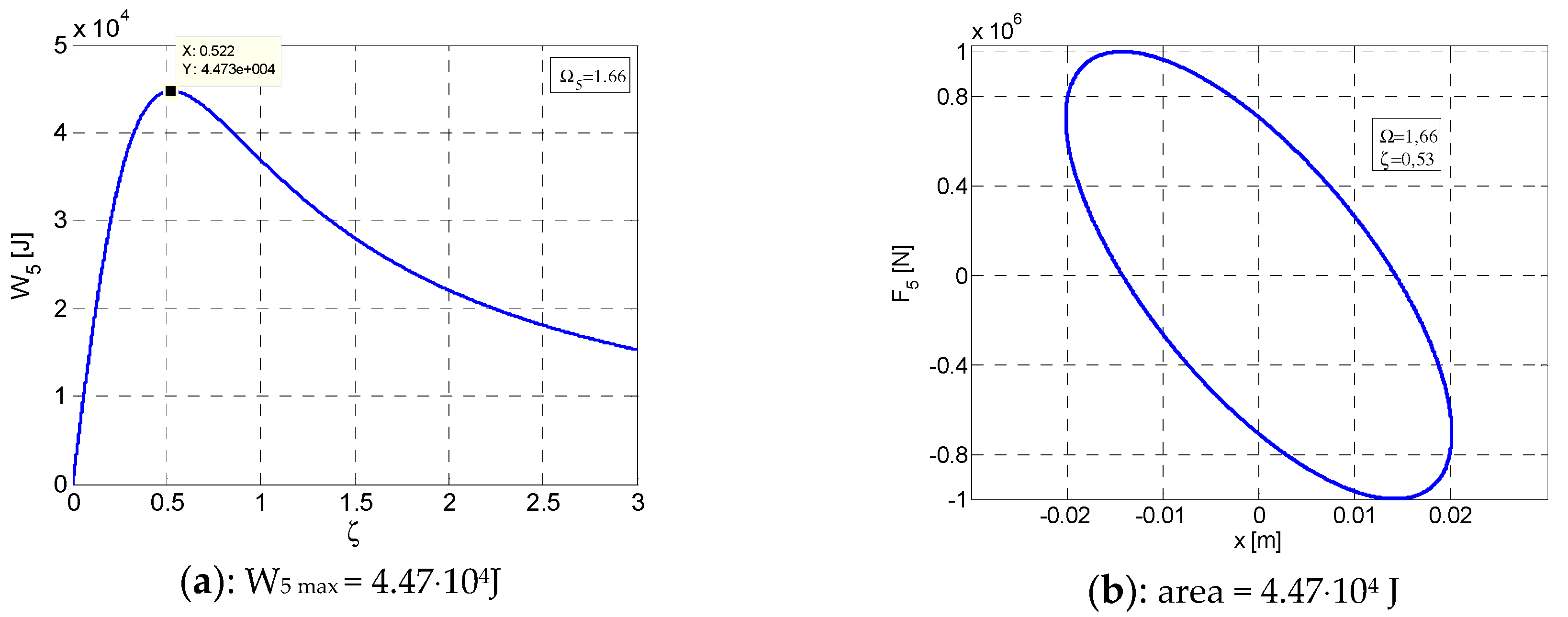

Figure 8.
Variation curves in post-resonance for W6max at Ω6 = 2 and ζ6 = 0.75. (a) Variation of W6 according to ζ. (b) Elliptic hysteretic loop F6–x. (c) Elliptic hysteretic loop Q6–x. x = [−0.01179 ÷ +0.01179].
Figure 8.
Variation curves in post-resonance for W6max at Ω6 = 2 and ζ6 = 0.75. (a) Variation of W6 according to ζ. (b) Elliptic hysteretic loop F6–x. (c) Elliptic hysteretic loop Q6–x. x = [−0.01179 ÷ +0.01179].
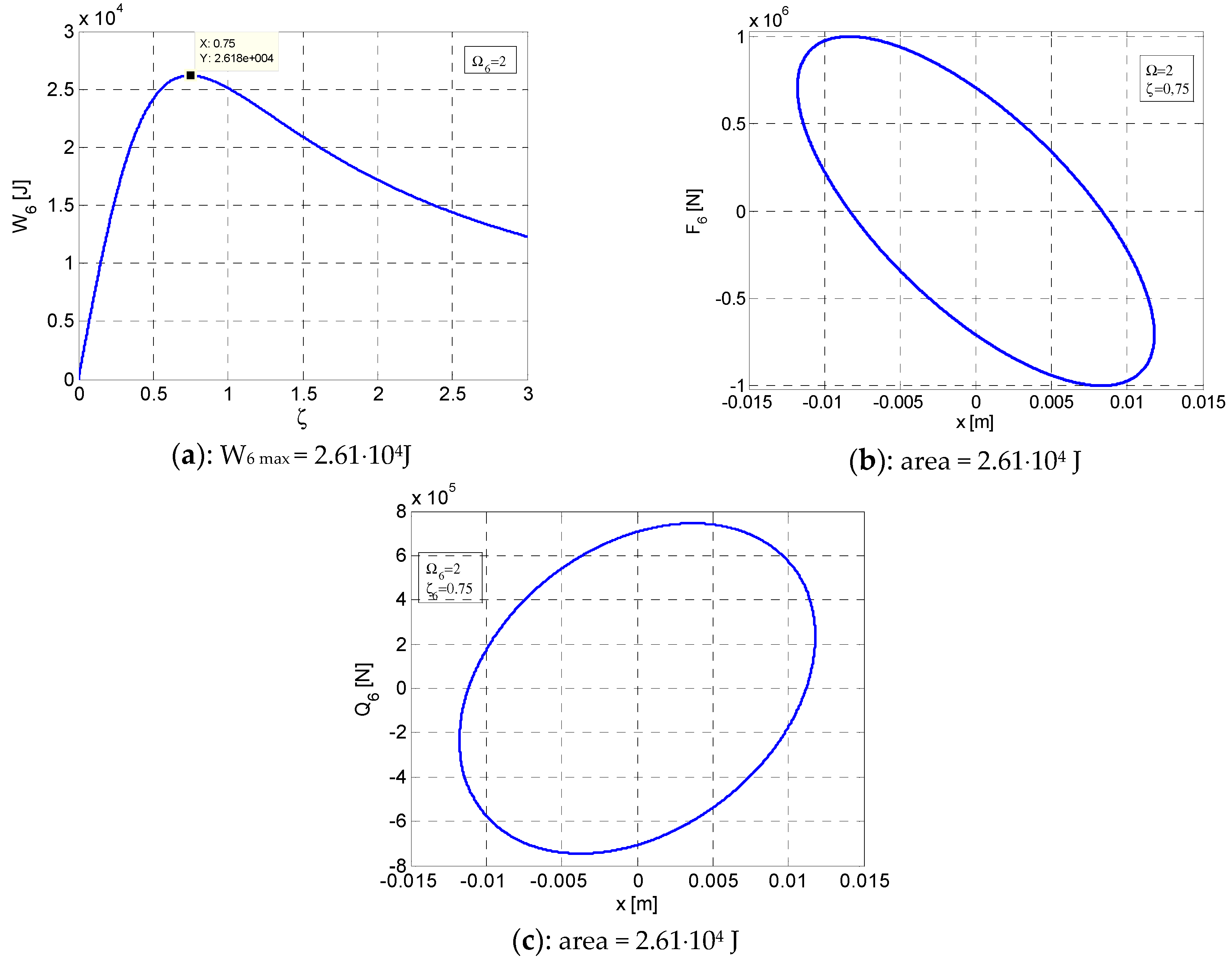
Figure 9.
Variation curves in post-resonance for W7max at Ω7 = 2.32 and ζ7 = 0.95. (a) Variation of W7 according to ζ. (b) Elliptic hysteretic loop F7–x. (c) Elliptic hysteretic loop Q7–x. x = [−0.008045 ÷ +0.008045].
Figure 9.
Variation curves in post-resonance for W7max at Ω7 = 2.32 and ζ7 = 0.95. (a) Variation of W7 according to ζ. (b) Elliptic hysteretic loop F7–x. (c) Elliptic hysteretic loop Q7–x. x = [−0.008045 ÷ +0.008045].
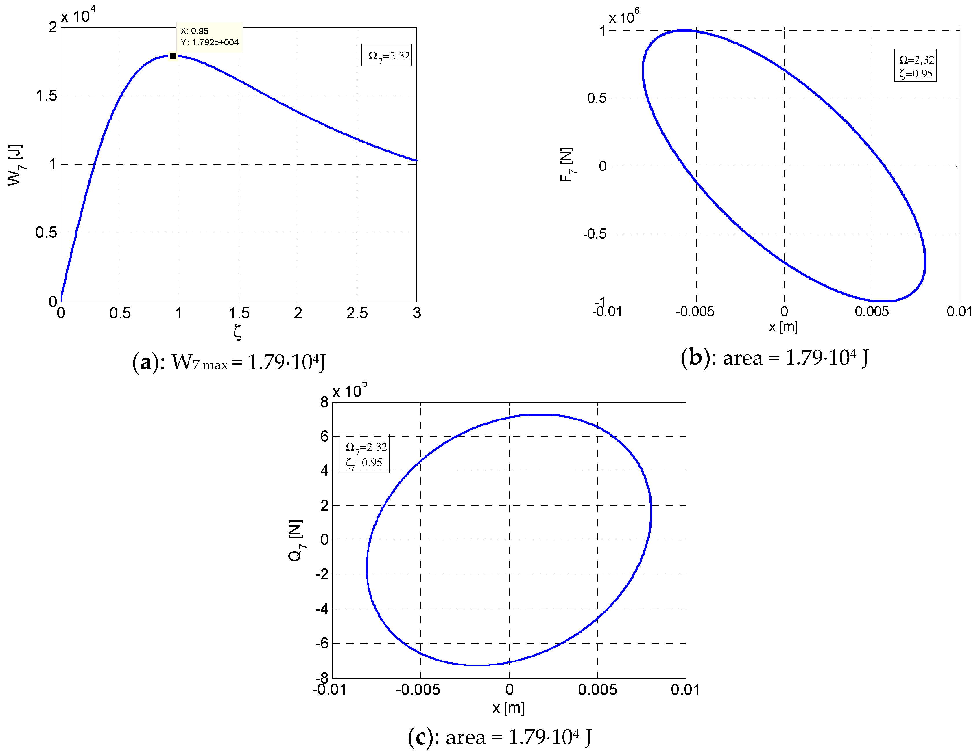
Figure 10.
Families of curves in post-resonance for the maximum values of the dissipated energy W4, W5, W6, and W7 at parameters (Ω4, ζ4), (Ω5, ζ5), (Ω6, ζ6), and (Ω7, ζ7). (a) Families of curves W parametrized by the discreet variable Ω. (b) The family of elliptical hysteretic loops F–x for the pair of variables Ω, ζ. (c) The family of elliptical hysteretic loops Q–x for the pair of variables Ω, ζ.

© 2019 by the author. Licensee MDPI, Basel, Switzerland. This article is an open access article distributed under the terms and conditions of the Creative Commons Attribution (CC BY) license (http://creativecommons.org/licenses/by/4.0/).
Share and Cite
MDPI and ACS Style
Bratu, P. Hysteretic Loops in Correlation with the Maximum Dissipated Energy, for Linear Dynamic Systems. Symmetry 2019, 11, 315. https://doi.org/10.3390/sym11030315
AMA Style
Bratu P. Hysteretic Loops in Correlation with the Maximum Dissipated Energy, for Linear Dynamic Systems. Symmetry. 2019; 11(3):315. https://doi.org/10.3390/sym11030315
Chicago/Turabian StyleBratu, Polidor. 2019. "Hysteretic Loops in Correlation with the Maximum Dissipated Energy, for Linear Dynamic Systems" Symmetry 11, no. 3: 315. https://doi.org/10.3390/sym11030315
Note that from the first issue of 2016, this journal uses article numbers instead of page numbers. See further details here.