Shewhart Attribute and Variable Control Charts Using Modified Multiple Dependent State Sampling


1
Department of Statistics, Faculty of Science, King Abdulaziz University, Jeddah 21551, Saudi Arabia
2
Department of Statistics, University of Veterinary and Animal Sciences, Lahore, Jhang campus, Lahore 54000, Pakistani
*
Author to whom correspondence should be addressed.
Symmetry 2019, 11(1), 53; https://doi.org/10.3390/sym11010053
Submission received: 4 December 2018
/
Revised: 25 December 2018
/
Accepted: 30 December 2018
/
Published: 5 January 2019
Abstract
:In this article, modified multiple dependent (or deferred) state sampling control charts for the attribute and the variable quality characteristics are presented. The proposed control charts are designed using the symmetry property of the normal distribution. The control chart coefficients are estimated through simulation at different levels of the parameters using the normal distribution. The proposed control chart scheme is evaluated by calculating the in-control average run lengths and out-of-control average run lengths. Tables are constructed for the selection of parameters for different control limit coefficients under several shift levels for the attribute data as well as the variable data. Examples are included for the practical application of the proposed control chart schemes. The proposed control chart scheme is also compared with the existing control charts. It has been observed that the proposed schemes are better in quick detection of the out-of-control processes.
1. Introduction
Process monitoring is an important tool of quality improvement or maintaining the current quality level. For example, the manufacturer earns its profit when the quality of the product is increased continuously and/or there is less variation in the current quality level. Both of these situations are intended to quantify for any change in the quality characteristic. Shewhart A. Walter introduced the technique of control charts during the 1920s, which is a graphical display with control limits generated from samples collected from the production process to indicate whether the process is in-control or out-of-control to prevent the scrapping of items. The basic idea of the control limits is still the same but a lot of literature is available to develop a robust technique and eventually to improve the performance of the control chart.
Ultimately, quick and early detection of change in any production process is the prime objective of the control chart, for which several sampling schemes have been proposed in the statistical control process [1]. Single sampling and double sampling schemes are the commonly used sampling schemes in which the decision for the in-control and out-of-control process is based upon the information obtained from the current sample and totally neglects the information from the aforementioned or the forthcoming samples [2]. The multiple dependent (or deferred) state (MDS) sampling scheme was introduced by [3] and is known as the conditional sampling scheme. In MDS sampling the declaration of the out-of-control process (not necessarily always) is made on the basis of not only the current sample information, but also the previous sample information. Several quality control researchers depend upon MDS sampling for the study of the processes [2]. Soundararajan and Vijayaraghavan [4] developed a MDS sampling plan for MDS-1 (0,2) type having minimum risks. Soundararajan and Vijayaraghavan [5] introduced a MDS sampling plan for MDS-() type having a smaller sample size. Govindaraju and Subramani [6] developed the MDS sampling plans for the minimum sum of the producer’s and the consumer’s risks using specific acceptable quality level and the limiting quality level. Balamurali and Jun [7] developed a MDS sampling plan for variable data using the normally distributed quality characteristics. Aslam et al. [8] used MDS sampling to develop the X-bar control chart based upon double control limits. Aslam et al. [9] proposed an attribute np control chart using MDS sampling. Balamurali et al. [2] developed a Bayesian multiple dependent state sampling plan for the Gamma–Poisson distribution. MDS sampling has been explored by many authors, including references [7,8,9,10,11,12,13,14,15].
Two types of control charts are available in the literature: attribute (p, np to monitor the fraction of non-conforming and c and are used to monitor the number of non-conformities etc.) charts are used when the quality characteristic is counted as pass or fail, conforming or non-conforming etc., and variable ( R, S etc.) control charts are applied when the quality characteristic is measureable as temperature, weight, height etc. Attribute control charts, which are widely accepted charts due to their simplicity in implementation, are used to categorize the items as good or defective by comparing them with the standard item, Montgomery [1]. Variable charts provide more information as compared to the attribute charts but involve more laborious calculation than just categorizing the items [1]. The average run length (ARL) is the most commonly used measure for performance evaluation of the control chart. It is defined as the average number of samples falling in the in-control limits until an out-of-control sample is indicated.
Both these types of quality characteristics have been explored under MDS sampling in this paper. The operation of a control chart using MDS sampling is based on the four control limits, namely two outer control limits and two inner control limits. The process is said to be in-control if the plotting statistic lies between two inner control limits and out-of-control if it lies outside the outer control limits. The process is considered as in-decision if some plotting statistic is between the outer and inner control limits. In this situation, the existing MDS sampling guide the practitioner to collect information from previous in-control subgroups. The process is declared to be in-control if a specified number of the previous subgroup are in-control, otherwise they are out-of-control. However, the proposed modified MDS sampling is more flexible than the existing MDS sampling, see Aslam et al. [9]. In the proposed MDS, the decision about in-control state is taken on the basis of previous in-control subgroups and allowing that a maximum of one subgroup may lie in between the outer and inner control limits. The MDS was introduced in the area of sampling plan by Govindaraju and Subramani [6].
According to the best of authors’ knowledge, no control chart using modified MDS has yet been proposed. Therefore, the Shewhart attribute and variable control charts are designed using modified MDS sampling in this paper. The proposed control will be helpful to test the hypothesis that the process mean is same with the alternative hypothesis that the process mean has changed. It is expected that the proposed control charts will be more efficient than the traditional Shewhart control charts and the existing control charts based on MDS sampling in terms of average run length. The efficiency of the proposed control charts will be given with the help of a simulation study and real examples.
The rest of the paper is organized as follows: the attribute chart using the modified MDS sampling is proposed in Section 2. The result of ARL performance for the proposed attribute chart is given in Section 3. Comparison of the proposed attribute chart with the existing attribute control chart is discussed in Section 4. In the second portion of the paper, the variable chart using the modified MDS sampling chart has been developed. Thus, the design of the variable MDS sampling is given in Section 5. The results of ARLs for the variable chart are given in Section 6. Comparison of the proposed variable chart with the existing variable control chart is discussed in Section 7.
2. Attribute Chart Using Modified Multiple Dependent State (MDS) Sampling
In this section, working of the proposed attribute chart using the modified MDS sampling will be explained. As mentioned earlier, in the proposed MDS, the decision about in-control state is taken on the basis of previous in-control subgroups and allowing that a maximum of one subgroup may lie in between the outer and inner control limits. The steps of the proposed control chart are as follows:
Step-1: Count the number of defectives from .
Step-2: If , the process is in-control. If or out-of-control, otherwise, go to Step-3.
Step-3: Declare the process is in control if m proceeding subgroups are in-control except in one sample where or .
By the usual MDS sampling scheme, the process is declared as in-control if m proceeding subgroups declared the process as in-control. Therefore, the use of the modified MDS sampling may be more flexible.
Let be the probability that an item becomes a defective when the process is in-control. Then, is the mean and is the variance of the number of defectives (denoted by D). Therefore, the four control limits of the proposed chart are:
The proposed attribute control chart contains two coefficients and , which will be determined by considering the in-control ARL.
Now, the probability that the process is declared as in-control under the modified MDS sampling is given as follows [16]:
It is to be noted here that the proposed attribute chart becomes the traditional Shewhart chart when = and = 1.
2.1. In-Control Process
Hence, the in-control ARL (denoted by ARL0) when is finally obtained by
where shows the number of defectives may 0, 1, …, n.
2.2. Shifted (or Out-Of-Control) Process
Hence, the out-of-control ARL (denoted by ARL1) when is finally obtained as
The performance of the proposed chart is assessed by computing the values of ARL, so the in-control ARL0 denoted by r0 is obtained as the average number of samples when the false alarm indicates for the specified values of the MDS sample parameter i. Here, it is to be noted that the larger values of the ARL0 are recommended as the process is in a situation of in-control, and no change occurs. For the specific values of ARL0 = 200, 300, and 370, the values of have been computed by running the R-code program using the simulation approach. This type of simulation approach is employed when the mean and other measures of the proposed chart are unavailable. Several researchers of the statistical process control used the simulation approach for numerical calculations of the proposed methodology including, for example, [17].
3. ARLs of the Attribute Chart Using Modified MDS Sampling
In Table 1 the control chart coefficients and are estimated for the MDS sampling parameter = 2, and 3. The performance of the proposed methodology is evaluated by calculating values, in which the smaller values show the early indication of false alarm [1]. The smaller the value of is, the better the performance of the proposed chart is. Thus, Table 1, Table 2 and Table 3 are generated for different process settings using different shift levels from 1.00 to 2.00. It can be observed that as the shift level increases, the ARL1 is going to decrease. This means that the larger shifts are addressed quickly, for example a shift of size 1.01 is detected with 188.49 samples on the average for = 2, r0 = 200 and , while a shift of 1.80 is detected with 2.52 samples for the same process settings. The same pattern can be observed for = 0.05 and = 0.10.
4. Comparison of the Proposed Chart with Existing MDS chart
In this section, the advantages of the proposed chart over the existing chart by [9] based on MDS sampling will be discussed. As mentioned earlier, the proposed attribute chart is equal to the [9] chart when . Therefore, using the same parameters and setting the ARL1 values from the proposed chart and [9], the results are reported in Table 4 for and = 300. A control chart having the smaller values of ARL1 of the same parameters is considered as the more efficient chart. From Table 4, it can be noted that the proposed control chart has smaller ARL1 as compared to the [9] chart. For instance, a shift of 1.20 is detected by an average of 50 samples, while the existing chart detects the same shift with an average of 43 samples. Figure 1 is presented for = 2, = 370 and . From Figure 1, it is clear that the ARL curve for is higher than the ARL curve when .
4.1. Simulation Study
In this section, the methodology of the proposed attribute control chart is explained for its practical use with the help of simulated data. The efficiency of the proposed control chart will be compared with existing Shewhart control charts based on single sampling and MDS sampling by [9]. For this simulation study, first, 20 observations were generated from in-control process with n = 205 and p0 = 0.10. Then, the next 20 observations were generated from the shifted process with n = 205, p1 = c*p0 where c = 1.25 from Table 2, ARL1 was 17.91, and the shift was detected on observation 17. The simulated data were 13, 25, 24, 21, 20, 19, 19, 22, 23, 22, 16, 26, 13, 19, 21, 24, 18, 18, 16, 18, 24, 32, 38, 18, 29, 20, 27, 22, 28, 28, 32, 25, 30, 25, 42, 24, 23, 24, 23, and 24. Figure 1 shows the simulated data of 40 observations, in which the process indicates an out-of-control situation after 20 + 15 = 35 samples. Thus, the proposed chart is effective in detecting a shift of 1.25 after 15 samples (a value of ARL1 from Table 3 for r0 = 370 and = 2). To compare the proposed control chart with the existing chart by [9], the values of statistic are also plotted on the control chart in Figure 2. By comparing Figure 2 with Figure 3, it can be noted that the existing control chart by [9] does not have the ability to detect the shift in the process. Figure 4 shows that the process is in-control. Similarly, the values of statistic are also plotted on the Shewhart control chart in Figure 4. From Figure 4, it can be observed that the Shewhart control chart does not detect the shift in the process. Therefore, the current chart is more efficient than two existing control charts in detecting quick shift in the manufacturing process.
4.2. An Industrial Example
Now the application of the proposed control is given on real data from the plastic parts manufacturing industry. According to [1] “a control chart is used to control the fraction nonconforming for a plastic part manufactured in an injection molding process”. Ten subgroups each of size 100 are taken from [1]. The number of non-confirming data is: = 10, 15, 31, 18, 24, 12, 23, 15, 8 and 8 being noted down and presented here. Figure 5 shows the control chart with k1 = 4.340957 and k2 = 3.092937, and the control chart limits are calculated as LCL1 = 0, LCL2 = 4, UCL2 = 27, and UCL1 = 32. From Figure 5, it can be noted that although the process is in a state of control, the 3rd, 9th and 10th sample are near the control limits, which may cause the shift in the process.
5. Variable Chart Using Modified MDS Sampling
In this section, the application of the variable MDS sampling will be described. The steps of the MDS sampling are:
Step-1: Compute from subgroup size .
Step-2: If , the process is in-control. If or the process is out-of-control, otherwise, go to Step-3.
Step-3: Declare the process is in control if m proceeding subgroups declared the process as in-control except in one sample where or .
In this section the construction of the control limits under the MDS sampling scheme is given. Let be the mean and be the standard deviation of the variable chart. Then, the four control limits of the proposed chart are:
5.1. In-Control Process
Now the probability that the process is in-control under the MDS sampling with the parameter m is given as follows:
5.2. Shifted (or Out-Of-Control) Process
Suppose now that the process mean has shifted from to .
6. ARLs of Variable Chart Using Modified MDS Sampling
In Table 5 the control chart coefficients and are estimated for the MDS sampling parameter = 2, and 3. The performance of the proposed methodology is evaluated by calculating values, in which the smaller values show the early indication of false alarm [1]. The smaller the value of the is, the better the performance of the proposed chart is. Thus, Table 5 and Table 6 are generated for different process settings using different shift levels from 0.01 to 0.90. It can be observed that as the shift level increases, the ARL1 is going to decrease. This means that the larger shifts are addressed quickly, for example a shift of size 0.05 is detected with 188.89 samples on average for = 2, r0 = 200, while a shift of 0.80 is detected with 4.25 samples for the same process settings. The same pattern can be observed for = 10.
7. Comparison of the Proposed Chart with Existing MDS Chart
In this section, the advantages of the proposed chart over the existing chart by [8] based on MDS sampling are presented. As mentioned earlier, the proposed attribute chart is equal to the [8] chart when . Therefore, using the same parameters and setting the ARL1 values from the proposed chart and [8], the results are reported in Table 4 for and = 300. A control chart having the smaller values of ARL1 of the same parameters is considered as the more efficient chart. From Table 4, it can be noted that the proposed control chart has a smaller ARL1 as compared to the [8] chart. For instance, a shift of 1.20 is detected by an average of 109 samples, while the existing chart detects the same shift with an average of 89 samples. Figure 6 is presented for = 2 and = 370. From Figure 6, it is clear that the ARL curve for is higher than the ARL curve when .
7.1. Simulation Study
In this section, the methodology of the proposed variable control chart is explained for its practical use with the help of simulated data. The efficiency of the proposed control chart will be compared with existing Shewhart control charts based on single sampling and MDS sampling by [8].
First, 20 observations were generated from in-control process with mean, = 0 and = 1. Then, the next 20 observations were generated from the shifted process with c*, where c = 0.40 from Table 7, ARL1 was 17.97, and the shift is detected on observation 17. The simulated data are not given here due to short space. Figure 7 shows the simulated data of 40 observations in which the process indicates an out-of-control situation after 20 + 17 = 37 samples. Thus, the proposed chart is effective in detecting a shift of 0.40 after 17 samples (a value of ARL1 from Table 6 for r0 = 200 and = 3).
To compare the proposed control chart with the existing chart by [8], the values of statistic are also plotted on a control chart in Figure 8. By comparing Figure 7 with Figure 8, it can be noted that the existing control chart by [8] does not have ability to detect the shift in the process. Figure 8 shows that the process is in-control. Similarly, the values of statistic are also plotted on the Shewhart control chart in Figure 9. From Figure 9, it can be observed that the Shewhart control chart does not detect the shift in the process. Therefore, the current chart is more efficient than two existing control charts in detecting quick shift in the manufacturing process.
7.2. An industrial Example
Now the application of the proposed control is given on real data from the automobile industry. A control chart is used to control the mean value inside diameter measurements (mm) for automobile engine piston rings. Twenty-five subgroups each of size 5 are taken from [1]. Figure 10 shows the control chart with two pairs of limits for the data. From Figure 10, it can be noted that although the process is in a state of control, sample 14 is near the control limits, which needs the attention of industrial engineers.
8. Conclusions
In this paper, a control chart using modified multiple dependent state sampling for attribute and variable data has been presented. The parameters of the proposed chart are estimated using several process settings. The performance of the proposed chart has been evaluated by the average run lengths at different shift levels. The comparative performance for the quick and early detection of the out-of-control process has also been studied. Practical application of the proposed charts has been given through examples for the elucidation of proposed methodology. It has been observed that the proposed charts are better than the existing Shewhart chart by comparing the ARLs of the shifted processes. The proposed control chart can be used for other probability models by transforming the variable of interest into symmetry form. The control chart measures will be different for other symmetric probability models. The proposed charts are a useful addition in the toolkit of quality control personnel. The proposed methodology can further be extended for some non-normal distributions.
Author Contributions
Conceived and designed the experiments, M.A., N.K., and M.A.; performed the experiments, M.A. and N.K.; analyzed the data, M.A. and N.K.; contributed reagents/materials/analysis tools, M.A.; wrote the paper, M.A.
Funding
This article was funded by the Deanship of Scientific Research (DSR) at King Abdulaziz University, Jeddah. The authors, therefore, acknowledge with thanks DSR technical and financial support.
Acknowledgments
The authors are deeply thankful to the editor and reviewers for their valuable suggestions to improve the quality of this manuscript.
Conflicts of Interest
The authors declare no conflicts of interest regarding this paper.
References
- Montgomery, D.C. Introduction to Statistical Quality Control, 6th ed.; John Wiley & Sons, Inc.: New York, NY, USA, 2009. [Google Scholar]
- Balamurali, S.; Jeyadurga, P.; Usha, M. Designing of Bayesian multiple deferred state sampling plan based on gamma–Poisson distribution. Am. J. Math. Manag. Sci. 2016, 35, 77–90. [Google Scholar] [CrossRef]
- Wortham, A.W.; Baker, R.C. Multiple deferred state sampling inspection. Int. J. Prod. Res. 1976, 14, 719–731. [Google Scholar] [CrossRef]
- Soundararajan, V.; Vijayaraghavan, R. On designing multiple deferred state sampling (MDS-1 (0, 2)) plans involving minimum risks. J. Appl. Stat. 1989, 16, 87–94. [Google Scholar] [CrossRef]
- Soundararajan, V.; Vijayaraghavan, R. Construction and selection of multiple dependent (deferred) state sampling plan. J. Appl. Stat. 1990, 17, 397–409. [Google Scholar] [CrossRef]
- Govindaraju, K.; Subramani, K. Selection of multiple deferred (dependent) state sampling plans for given acceptable quality level and limiting quality level. J. Appl. Stat. 1993, 20, 423–428. [Google Scholar] [CrossRef]
- Balamurali, S.; Jun, C.-H. Multiple dependent state sampling plans for lot acceptance based on measurement data. Eur. J. Oper. Res. 2007, 180, 1221–1230. [Google Scholar] [CrossRef]
- Aslam, M.; Khan, N.; Jun, C.-H. A Multiple Dependent State Control Chart Based on Double Control Limit. Res. J. Appl. Sci. Eng. Technol. 2014, 7, 4490–4493. [Google Scholar] [CrossRef]
- Aslam, M.; Nazir, A.; Jun, C.-H. A new attribute control chart using multiple dependent state sampling. Trans. Inst. Meas. Control 2015, 37, 569–576. [Google Scholar] [CrossRef]
- Zhou, W.; Wan, Q.; Zheng, Y.; Zhou, Y.-W. A joint-adaptive np control chart with multiple dependent state sampling scheme. Commun. Stat. Theory Methods 2017, 46, 6967–6979. [Google Scholar] [CrossRef]
- Yan, A.; Liu, S.; Dong, X. Designing a multiple dependent state sampling plan based on the coefficient of variation. SpringerPlus 2016, 5, 1447. [Google Scholar] [CrossRef] [PubMed]
- Aslam, M.; Azam, M.; Khan, N.; Jun, C.-H. A control chart for an exponential distribution using multiple dependent state sampling. Qual. Quant. 2015, 49, 455–462. [Google Scholar] [CrossRef]
- Aslam, M.; Azam, M.; Jun, C.-H. Multiple dependent state sampling plan based on process capability index. J. Test. Eval. 2013, 41, 1–7. [Google Scholar] [CrossRef]
- Kuralmani, V.; Govlndaraju, K. Selection of multiple deferred (dependent) state sampling plans. Commun. Stat. Theory Methods 1992, 21, 1339–1366. [Google Scholar] [CrossRef]
- Vaerst, R. A procedure to construct multiple deferred state sampling plan. Methods Oper. Res. 1982, 37, 477–485. [Google Scholar]
- Govindaraju, K.; Lai, C. A modified ChSP-1 chain sampling plan, MChSP-1, with very small sample sizes. Am. J. Math. Manag. Sci. 1998, 18, 343–358. [Google Scholar] [CrossRef]
- Chananet, C.; Sukparungsee, S.; Areepong, Y. The ARL of EWMA chart for monitoring ZINB model using Markov chain approach. Int. J. Appl. Phys. Math. 2014, 4, 236. [Google Scholar] [CrossRef]
Figure 1.
The ARLs curves when = 2 and .

Figure 2.
Control chart for the proposed chart using the simulated data for p0 = 0.10 and r0 = 370.

Figure 3.
Control chart for the MDS sampling using the simulated data for p0 = 0.10 and r0 = 370.

Figure 4.
Shewhart control chart for the single chart using the simulated data for p0 = 0.10 and r0 = 370.
Figure 4.
Shewhart control chart for the single chart using the simulated data for p0 = 0.10 and r0 = 370.
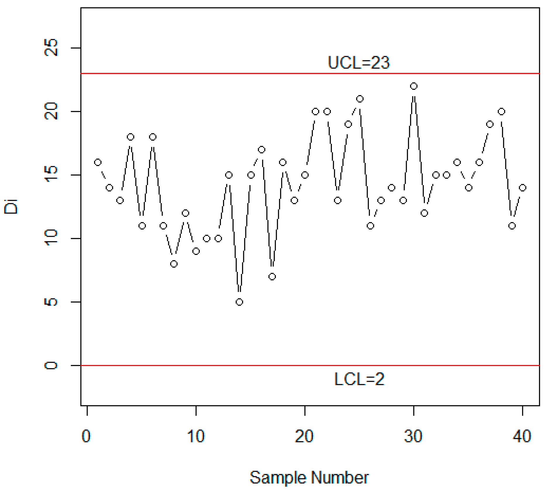
Figure 5.
Attribute control chart for the example [1].
Figure 5.
Attribute control chart for the example [1].
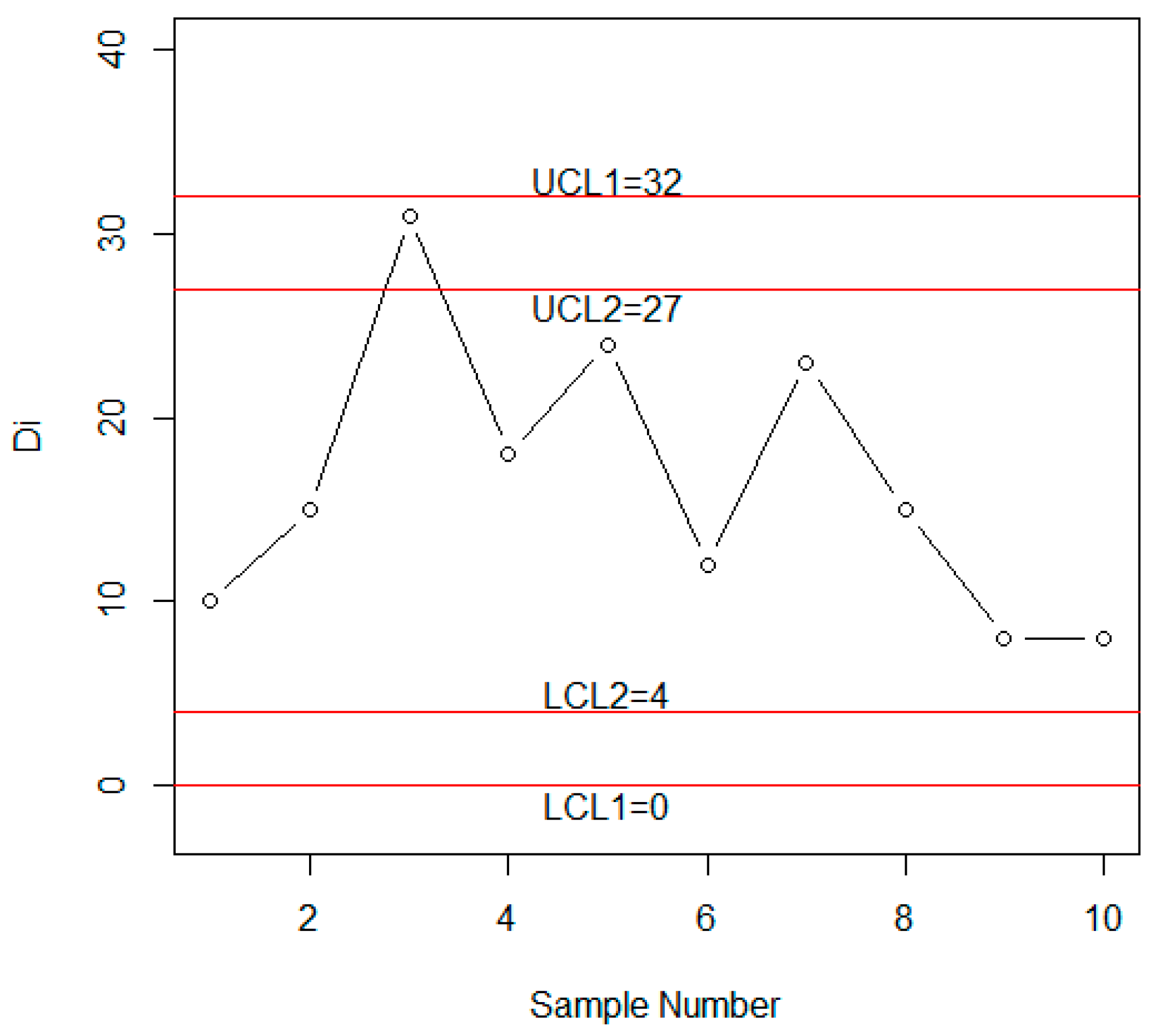
Figure 6.
The ARLs curve when = 2 and = 370.

Figure 7.
Control chart for the proposed chart using the simulated data for n = 10 and r0 = 370.
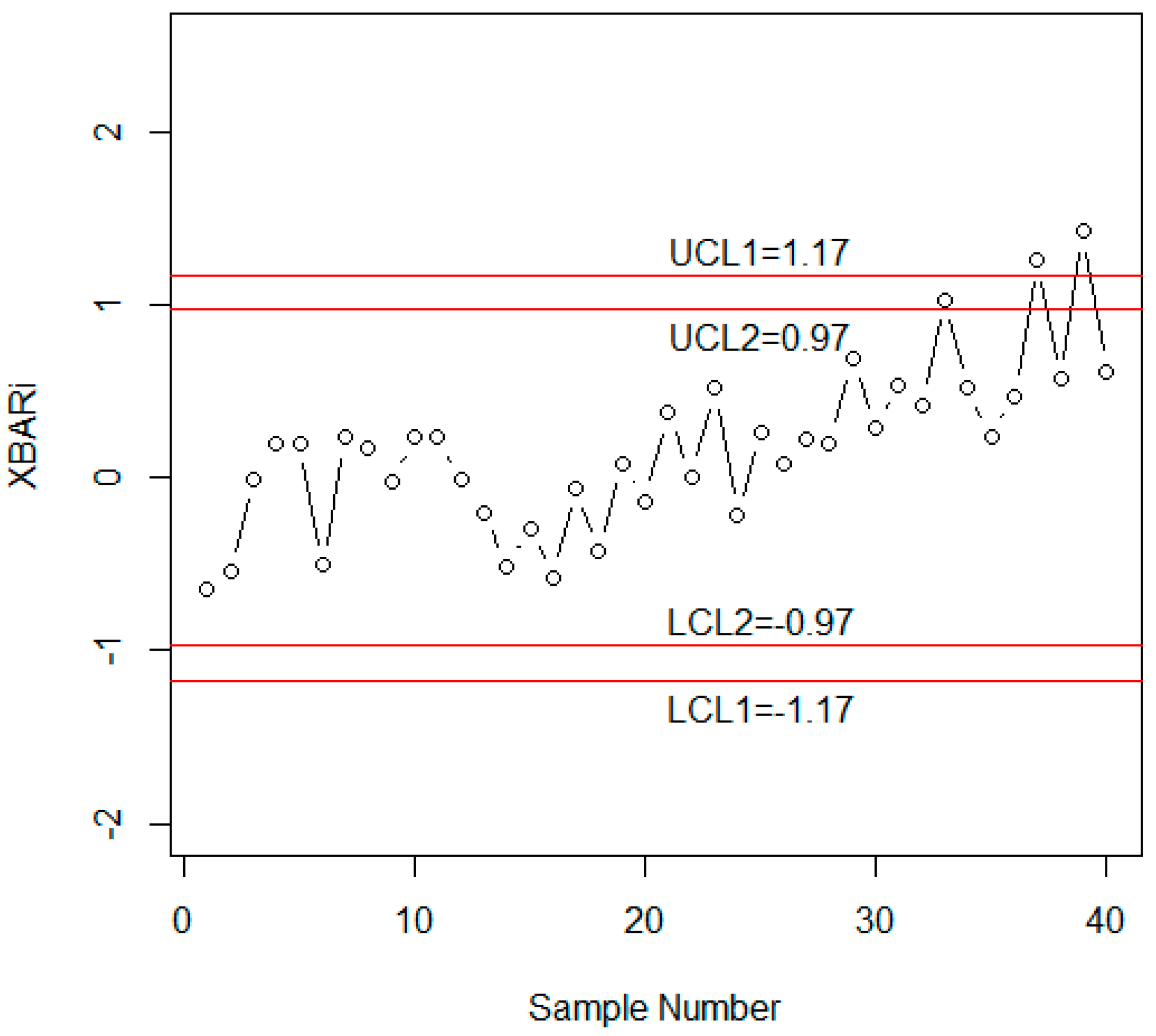
Figure 8.
Control chart for the MDS chart using the simulated data for n = 10 and r0 = 370.

Figure 9.
Shewhart Control chart for the Single chart using the simulated data for n = 10 and r0 = 370.
Figure 9.
Shewhart Control chart for the Single chart using the simulated data for n = 10 and r0 = 370.

Figure 10.
Variable control chart for the data given in [1].
Figure 10.
Variable control chart for the data given in [1].


Table 1.
The (ARL) values of the attribute chart for = 0.01.
| = 2 | = 3 | |||||
|---|---|---|---|---|---|---|
| 201.7800 | 301.5360 | 370.6202 | 200.9965 | 305.2319 | 373.4875 | |
| 4.8498 | 3.4960 | 3.6292 | 5.1498 | 3.7202 | 3.9085 | |
| 2.9614 | 3.4723 | 3.5639 | 3.6066 | 3.4506 | 3.4507 | |
| n | 810 | 900 | 880 | 680 | 920 | 900 |
| Shift | ||||||
| 1.00 | 201.78 | 301.54 | 370.62 | 201.00 | 305.23 | 373.49 |
| 1.01 | 188.49 | 273.78 | 339.37 | 209.70 | 276.88 | 342.11 |
| 1.03 | 163.20 | 224.71 | 281.99 | 225.50 | 226.49 | 283.89 |
| 1.05 | 140.34 | 183.98 | 232.62 | 237.95 | 184.58 | 233.43 |
| 1.07 | 120.23 | 150.71 | 191.33 | 245.73 | 150.38 | 191.13 |
| 1.10 | 95.16 | 112.31 | 142.83 | 246.62 | 111.07 | 141.53 |
| 1.13 | 75.49 | 84.47 | 107.28 | 234.44 | 82.76 | 105.36 |
| 1.15 | 64.88 | 70.29 | 89.09 | 220.41 | 68.43 | 86.97 |
| 1.17 | 55.92 | 58.79 | 74.32 | 203.29 | 56.88 | 72.11 |
| 1.20 | 45.01 | 45.42 | 57.16 | 174.96 | 43.54 | 54.96 |
| 1.25 | 31.90 | 30.32 | 37.84 | 129.61 | 28.64 | 35.85 |
| 1.30 | 23.11 | 20.89 | 25.83 | 93.29 | 19.46 | 24.14 |
| 1.40 | 12.90 | 10.83 | 13.14 | 48.19 | 9.84 | 11.97 |
| 1.50 | 7.76 | 6.25 | 7.43 | 26.04 | 5.57 | 6.63 |
| 1.70 | 3.45 | 2.74 | 3.12 | 9.04 | 2.40 | 2.73 |
| 1.80 | 2.52 | 2.05 | 2.28 | 5.81 | 1.80 | 2.00 |
| 2.00 | 1.60 | 1.38 | 1.48 | 2.85 | 1.25 | 1.33 |
Table 2.
The ARL values of the attribute chart for = 0.05.
| = 2 | = 3 | |||||
|---|---|---|---|---|---|---|
| 200.4457 | 301.5679 | 371.4451 | 200.1407 | 300.1609 | 370.1112 | |
| 3.5377 | 4.5655 | 4.3772 | 6.1016 | 3.5814 | 5.6740 | |
| 2.9214 | 2.9908 | 3.1114 | 2.9065 | 3.0666 | 3.1167 | |
| n | 290 | 275 | 270 | 225 | 395 | 315 |
| Shift | ||||||
| 1.00 | 200.45 | 301.57 | 371.45 | 200.14 | 300.16 | 370.11 |
| 1.01 | 177.09 | 266.99 | 328.98 | 180.06 | 259.69 | 324.69 |
| 1.03 | 138.23 | 209.93 | 258.33 | 146.05 | 193.00 | 250.51 |
| 1.05 | 108.23 | 165.99 | 203.62 | 118.95 | 143.30 | 194.32 |
| 1.07 | 85.20 | 132.11 | 161.37 | 97.33 | 106.92 | 151.76 |
| 1.10 | 60.28 | 95.04 | 115.23 | 72.75 | 69.98 | 106.19 |
| 1.13 | 43.37 | 69.47 | 83.54 | 55.03 | 46.82 | 75.56 |
| 1.15 | 35.17 | 56.86 | 67.99 | 45.98 | 36.27 | 60.76 |
| 1.17 | 28.73 | 46.85 | 55.71 | 38.61 | 28.39 | 49.20 |
| 1.20 | 21.52 | 35.47 | 41.82 | 29.98 | 20.04 | 36.29 |
| 1.25 | 13.79 | 22.99 | 26.73 | 20.12 | 11.78 | 22.51 |
| 1.30 | 9.23 | 15.43 | 17.71 | 13.87 | 7.35 | 14.47 |
| 1.40 | 4.68 | 7.65 | 8.57 | 7.12 | 3.40 | 6.60 |
| 1.50 | 2.76 | 4.27 | 4.69 | 4.05 | 1.96 | 3.46 |
| 1.70 | 1.43 | 1.87 | 1.98 | 1.81 | 1.13 | 1.50 |
| 1.80 | 1.20 | 1.44 | 1.50 | 1.42 | 1.04 | 1.21 |
| 2.00 | 1.04 | 1.10 | 1.12 | 1.09 | 1.00 | 1.03 |
Table 3.
The ARL values of the attribute chart for = 0.10.
| = 2 | = 3 | |||||
|---|---|---|---|---|---|---|
| 200.8375 | 301.9349 | 370.9957 | 200.0664 | 300.0649 | 374.3649 | |
| 6.0760 | 3.7269 | 4.9422 | 3.9412 | 3.3411 | 3.6377 | |
| 2.7771 | 3.4279 | 2.9897 | 2.9031 | 3.3107 | 3.4403 | |
| n | 100 | 85 | 205 | 290 | 370 | 140 |
| Shift | ||||||
| 1.00 | 200.84 | 301.93 | 371.00 | 200.07 | 300.06 | 374.36 |
| 1.01 | 182.99 | 275.08 | 327.06 | 177.38 | 249.31 | 322.69 |
| 1.03 | 151.61 | 226.98 | 250.60 | 134.45 | 167.37 | 241.28 |
| 1.05 | 125.60 | 186.56 | 190.56 | 99.38 | 111.46 | 182.06 |
| 1.07 | 104.27 | 153.23 | 145.03 | 72.94 | 74.92 | 138.68 |
| 1.10 | 79.38 | 114.47 | 97.35 | 46.14 | 42.58 | 93.83 |
| 1.13 | 61.04 | 86.18 | 66.57 | 29.74 | 25.26 | 64.82 |
| 1.15 | 51.54 | 71.72 | 52.25 | 22.48 | 18.27 | 51.22 |
| 1.17 | 43.72 | 59.97 | 41.39 | 17.17 | 13.47 | 40.83 |
| 1.20 | 34.48 | 46.28 | 29.66 | 11.71 | 8.83 | 29.52 |
| 1.25 | 23.76 | 30.80 | 17.74 | 6.56 | 4.81 | 17.91 |
| 1.30 | 16.83 | 21.13 | 11.14 | 3.97 | 2.93 | 11.40 |
| 1.40 | 9.11 | 10.83 | 5.02 | 1.88 | 1.51 | 5.30 |
| 1.50 | 5.39 | 6.17 | 2.70 | 1.24 | 1.11 | 2.93 |
| 1.70 | 2.42 | 2.65 | 1.30 | 1.01 | 1.00 | 1.41 |
| 1.80 | 1.82 | 1.96 | 1.11 | 1.00 | 1.00 | 1.17 |
| 2.00 | 1.27 | 1.32 | 1.01 | 1.00 | 1.00 | 1.02 |
Table 4.
Comparison in ARLs when = 0.01, and = 3.
| Existing MDS Chart | Proposed Chart | Existing MDS Chart | Proposed Chart | |
|---|---|---|---|---|
| Shift | ||||
| 1.00 | 301.13 | 305.23 | 372.32 | 300.10 |
| 1.01 | 273.31 | 276.88 | 355.19 | 271.30 |
| 1.03 | 225.13 | 226.49 | 316.12 | 219.32 |
| 1.05 | 185.76 | 184.58 | 274.42 | 175.62 |
| 1.07 | 153.77 | 150.38 | 233.71 | 139.99 |
| 1.10 | 116.71 | 111.07 | 179.26 | 99.58 |
| 1.13 | 89.53 | 82.76 | 135.24 | 71.31 |
| 1.15 | 75.49 | 68.43 | 111.65 | 57.45 |
| 1.17 | 63.98 | 56.88 | 92.15 | 46.57 |
| 1.20 | 50.38 | 43.54 | 69.32 | 34.44 |
| 1.25 | 34.65 | 28.64 | 43.89 | 21.62 |
| 1.30 | 24.53 | 19.46 | 28.62 | 14.23 |
| 1.40 | 13.28 | 9.84 | 13.48 | 7.06 |
| 1.50 | 7.89 | 5.57 | 7.25 | 4.11 |
| 1.70 | 3.53 | 2.40 | 2.96 | 2.04 |
| 1.80 | 2.61 | 1.80 | 2.17 | 1.65 |
| 2.00 | 1.68 | 1.25 | 1.45 | 1.27 |
Table 5.
The ARL values of the variable chart for .
| = 2 | = 3 | |||||
|---|---|---|---|---|---|---|
| 201.3894 | 300.2447 | 370.9500 | 200.2556 | 301.5969 | 376.9614 | |
| 3.2778 | 3.4290 | 3.3808 | 3.4319 | 3.3473 | 3.4785 | |
| 2.9806 | 3.0730 | 3.2267 | 2.9495 | 3.3291 | 3.2531 | |
| c | ||||||
| 0.00 | 201.39 | 300.24 | 370.95 | 200.26 | 301.60 | 376.96 |
| 0.01 | 200.86 | 299.41 | 369.86 | 199.72 | 300.69 | 375.80 |
| 0.03 | 196.72 | 292.88 | 361.31 | 195.54 | 293.63 | 366.77 |
| 0.05 | 188.89 | 280.56 | 345.24 | 187.64 | 280.34 | 349.81 |
| 0.07 | 178.14 | 263.71 | 323.38 | 176.79 | 262.31 | 326.82 |
| 0.10 | 158.56 | 233.27 | 284.21 | 157.08 | 230.07 | 285.86 |
| 0.13 | 137.46 | 200.79 | 242.87 | 135.88 | 196.18 | 242.97 |
| 0.15 | 123.66 | 179.74 | 216.35 | 122.04 | 174.49 | 215.64 |
| 0.17 | 110.59 | 159.94 | 191.57 | 108.95 | 154.28 | 190.23 |
| 0.20 | 92.83 | 133.26 | 158.48 | 91.20 | 127.36 | 156.51 |
| 0.25 | 68.68 | 97.39 | 114.54 | 67.12 | 91.76 | 112.12 |
| 0.30 | 50.73 | 71.09 | 82.78 | 49.30 | 66.13 | 80.34 |
| 0.40 | 28.23 | 38.64 | 44.19 | 27.07 | 35.15 | 42.20 |
| 0.50 | 16.36 | 21.87 | 24.61 | 15.45 | 19.52 | 23.13 |
| 0.70 | 6.33 | 8.05 | 8.82 | 5.79 | 7.01 | 8.06 |
| 0.80 | 4.25 | 5.25 | 5.69 | 3.83 | 4.55 | 5.14 |
| 0.90 | 3.01 | 3.61 | 3.87 | 2.69 | 3.13 | 3.47 |
Table 6.
The ARL values of the variable chart for .
| 200.2658 | 300.8521 | 371.6013 | 200.6461 | 300.0891 | 370.2289 | |
|---|---|---|---|---|---|---|
| 4.241692 | 3.865157 | 3.706407 | 4.389848 | 4.384344 | 3.524029 | |
| 2.81188 | 2.958272 | 3.082647 | 2.814882 | 2.941529 | 3.189481 | |
| c | ||||||
| 0 | 200.27 | 300.85 | 371.60 | 200.65 | 300.09 | 370.23 |
| 0.01 | 199.38 | 299.35 | 369.50 | 199.75 | 298.64 | 368.00 |
| 0.03 | 192.55 | 287.79 | 353.39 | 192.84 | 287.48 | 350.99 |
| 0.05 | 180.07 | 266.91 | 324.63 | 180.22 | 267.26 | 320.85 |
| 0.07 | 163.87 | 240.21 | 288.51 | 163.83 | 241.26 | 283.34 |
| 0.1 | 136.85 | 196.73 | 231.19 | 136.51 | 198.60 | 224.71 |
| 0.13 | 110.86 | 156.13 | 179.37 | 110.25 | 158.39 | 172.61 |
| 0.15 | 95.41 | 132.57 | 150.05 | 94.64 | 134.87 | 143.52 |
| 0.17 | 81.78 | 112.14 | 125.10 | 80.88 | 114.36 | 119.00 |
| 0.2 | 64.70 | 87.03 | 95.08 | 63.65 | 89.01 | 89.80 |
| 0.25 | 43.90 | 57.29 | 60.54 | 42.69 | 58.71 | 56.65 |
| 0.3 | 30.14 | 38.23 | 39.14 | 28.87 | 39.11 | 36.40 |
| 0.4 | 14.92 | 17.97 | 17.34 | 13.75 | 18.10 | 16.07 |
| 0.5 | 7.93 | 9.13 | 8.37 | 6.98 | 8.92 | 7.82 |
| 0.7 | 2.84 | 3.06 | 2.65 | 2.36 | 2.78 | 2.56 |
| 0.8 | 1.95 | 2.04 | 1.78 | 1.63 | 1.84 | 1.74 |
| 0.9 | 1.47 | 1.52 | 1.35 | 1.27 | 1.37 | 1.34 |
Table 7.
Comparison in ARLs when = 10 and = 3.
| Existing MDS Chart | Proposed Chart | |
|---|---|---|
| c | ||
| 1.00 | 370.77 | 370.23 |
| 1.01 | 368.95 | 368.00 |
| 1.03 | 354.95 | 350.99 |
| 1.05 | 329.63 | 320.85 |
| 1.07 | 297.20 | 283.34 |
| 1.10 | 244.27 | 224.71 |
| 1.13 | 194.70 | 172.61 |
| 1.15 | 165.86 | 143.52 |
| 1.17 | 140.80 | 119.00 |
| 1.20 | 109.93 | 89.80 |
| 1.25 | 73.21 | 56.65 |
| 1.30 | 49.53 | 36.40 |
| 1.40 | 24.08 | 16.07 |
| 1.50 | 12.74 | 7.82 |
| 1.70 | 4.56 | 2.56 |
| 1.80 | 3.06 | 1.74 |
| 2.00 | 2.21 | 1.34 |
© 2019 by the authors. Licensee MDPI, Basel, Switzerland. This article is an open access article distributed under the terms and conditions of the Creative Commons Attribution (CC BY) license (http://creativecommons.org/licenses/by/4.0/).
Share and Cite
MDPI and ACS Style
Aslam, M.; Khan, N.; Albassam, M. Shewhart Attribute and Variable Control Charts Using Modified Multiple Dependent State Sampling. Symmetry 2019, 11, 53. https://doi.org/10.3390/sym11010053
AMA Style
Aslam M, Khan N, Albassam M. Shewhart Attribute and Variable Control Charts Using Modified Multiple Dependent State Sampling. Symmetry. 2019; 11(1):53. https://doi.org/10.3390/sym11010053
Chicago/Turabian StyleAslam, Muhammad, Nasrullah Khan, and Mohammed Albassam. 2019. "Shewhart Attribute and Variable Control Charts Using Modified Multiple Dependent State Sampling" Symmetry 11, no. 1: 53. https://doi.org/10.3390/sym11010053
Note that from the first issue of 2016, this journal uses article numbers instead of page numbers. See further details here.