Anti-Cavitation Design of the Symmetric Leading-Edge Shape of Mixed-Flow Pump Impeller Blades

1
Beijing Engineering Research Center of Safety and Energy Saving Technology for Water Supply Network System, China Agricultural University, Beijing 100083, China
2
College of Water Resources and Civil Engineering, China Agricultural University, Beijing 100083, China
3
Department of Energy and Power Engineering, Tsinghua University, Beijing 100084, China
*
Author to whom correspondence should be addressed.
Symmetry 2019, 11(1), 46; https://doi.org/10.3390/sym11010046
Submission received: 29 November 2018
/
Revised: 24 December 2018
/
Accepted: 26 December 2018
/
Published: 3 January 2019
(This article belongs to the Special Issue Broken Symmetries, Hydrodynamics and Rare Fluctuations)
Abstract
:Mixed-flow pumps compromise large flow rate and high head in fluid transferring. Long-axis mixed-flow pumps with radial–axial “spacing” guide vanes are usually installed deeply under water and suffer strong cavitation due to strong environmental pressure drops. In this case, a strategy combining the Diffusion-Angle Integral Design method, the Genetic Algorithm, and the Computational Fluid Dynamics method was used for optimizing the mixed-flow pump impeller. The Diffusion-Angle Integral Design method was used to parameterize the leading-edge geometry. The Genetic Algorithm was used to search for the optimal sample. The Computational Fluid Dynamics method was used for predicting the cavitation performance and head–efficiency performance of all the samples. The optimization designs quickly converged and got an optimal sample. This had an increased value for the minimum pressure coefficient, especially under off-design conditions. The sudden pressure drop around the leading-edge was weakened. The cavitation performance within the 0.5–1.2 Qd flow rate range, especially within the 0.62–0.78 Qd and 1.08–1.20 Qd ranges, was improved. The head and hydraulic efficiency was numerically checked without obvious change. This provided a good reference for optimizing the cavitation or other performances of bladed pumps.
1. Introduction
Cavitation is a liquid–gas phase change phenomenon which happens in the liquid medium when pressure drops below the saturation pressure [1]. Traveling cavitation vapour bubbles collapse immediately while going into high pressure sites [2]. The collapsing bubble may release shock waves and form re-entrant jets. These waves and jets cause noise, pressure pulsation, and vibration [3,4]. If cavitation happens near the surfaces of materials, the shock waves, re-entrant jets, and following rigid particles [5] cause material damage, like spotted erosion [6]. In pumps, cavitation was highly focused on in the past decades [7]. Cavitation-damaged pump impellers have bad performance and work in an unstable and insecure situation [8,9]. Thus, reducing cavitation scale or delaying cavitation inception is necessary in design. Cavitation in pumps occurs mainly in the leading-edge cavitation style because the impeller blade leading-edge is usually the lowest-pressure site [7]. The collapse of a bubble or cavity directly shocks the blade surface and induces cavitation erosion [10].
Improving cavitation performance or reducing cavitation scale is always on the research frontier. There are three main approaches: Direct interference, indirect influence, and cavitation-site redesign. Susan-Resiga et al. [11] used water jets to interfere with the vortex rope, and their results show that the low-pressure region inside the rope can be effectively diminished. Yang et al. [12] applied eight alternating long and short blades, instead of the original six same-length blades, in a centrifugal pump. This enlarged the original passing area, making it have a relatively higher pressure than before. Yao et al. [13] also increased the passing area of the Francis turbine for a higher pressure at the runner outlet. These methods may reduce the energy performance, so further checks and improvements are needed. Liu et al. [14] directly redesigned the leading-edge position of the centrifugal pump impeller blade. The lowest-pressure region was removed to an upstream location with a higher pressure value. However, the performance change cannot be ignored. The cavitation improvements above were mainly about large-scale cavitation. However, the cavitation inception has received little attention. In this study of a mixed-flow pump case, the cavitation inception performance becomes the optimization target. Optimization can be used to improve the performance of pumps. The most common optimization works in pumps and other hydraulic turbomachinery improved the efficiency by adjusting impeller geometry, including blade angles and meridional shape parameters [15,16,17]. When considering the optimization of cavitation performance, geometry control and searching were also effective. However, pump head and efficiency were sensitive to geometry [18,19]. The alternating checks of cavitation and head–efficiency increased the complexity of work. It is necessary to find a simpler way for parameterization of the blade, especially at the impeller blade leading-edge. A reasonable optimization method, prediction method, and decision-making strategy are also crucial.
In this study, the optimization design work was conducted on a mixed-flow pump impeller with consideration of the downstream vane diffuser. The Diffusion-Angle Integral (DI) method [20] was used to parameterize the leading-edge geometry, which is important for cavitation inception. The Genetic Algorithm (GA) was used for searching for the optimal sample. A Computational Fluid Dynamics (CFD) solver was used for predicting the cavitation performance and head–efficiency performance of all the samples. Based on this combination strategy, the cavitation performance was improved for a better operation stability and safety.
2. Mixed-Flow Pump Object
3. Mathematical Methods
3.1. Brief Introduction of the Diffusion-Angle Integral Method
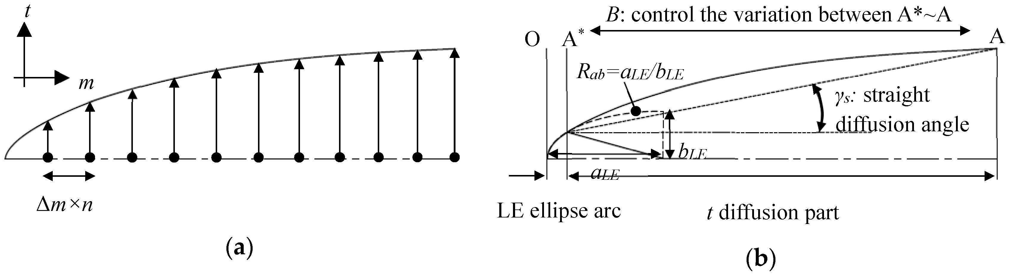
The Diffusion-Angle Integral (DI) method [20] was specifically used to parameterize the leading-edge geometry (thickness). Traditionally, the leading-edge geometry was controlled by multiple points with the connection of a B-spline, as shown in Figure 2a. Under the 2D t–m coordinate where t denotes thickness and m denotes the mean line, Δm-interval points were set to control the t distribution along the m direction. If the number of point n is small, the geometry cannot be described well. If the number of point n is big, optimization will be complex with too many parameters.
Therefore, the DI method was introduced based on a geometry deconstruction. The blade profile can be deconstructed into five parts, including the leading-edge (LE) ellipse arc, t diffusion part, t transition part, t shrinking part, and trailing-edge (TE). As shown in Figure 2b, point A, which is between the t diffusion part and t transition part, should be determined. Then, the LE ellipse arc and the t diffusion part, which are quickly changing on t, become the design region. Point A* is set to divide the LE ellipse arc and the t diffusion part. Five steps can be executed in sequence: (a) Giving the long–short axis ratio Rab = aLE/bLE of the LE ellipse arc, (b) scaling the leading-edge elliptical-arc to the arc based on Rab, (c) giving the straight thickness diffusion angle γs (unit: degree) and calculating the leading-edge arc (scaled) radius rLE, (d) giving the coefficient B of the thickness integration expression and integrating out the thickness distribution in the thickness diffusion part, and (e) rescaling the leading-edge arc and the integrated thickness back to the elliptical-arc-scale based on Rab.
Based on the steps above, the LE ellipse arc can be calculated under coordinate scaling:
where tA is the thickness at point A and mA is the m position at point A. Then, the increasing of t between A* and A can be integrated by
where mA* is the m position at point A*, Cs is the scale factor, and γ(m) is the thickness integral expression which can be expressed in the following form:
Thus, the variation law between A and A* can be simply and well controlled by the coefficient B. The number of design parameters was simplified to three by keeping an accurate description of t along m.
3.2. Genetic Algorithm and Setup
The Genetic Algorithm (GA), which is a nature-inspired optimization algorithm, can find better samples generation by generation after setting a fitness function [21]. It imitates biological evolution by treating samples as individuals. Certain quantities of individuals should be created. Their properties as fitness functions need to be carefully checked to judge the best and worst individuals. The best individual in each generation is copied and the worst one is eliminated. The remaining individuals crossover and mutate in a certain probability. Thus, the GA always finds better results and can escape from local-best traps. In this case, the GA was used for optimal impeller geometry. A cavitation inception number σ was set as the optimization target:
where pref and vref are the reference pressure and velocity at the impeller inlet, respectively. pv is the saturation pressure. ρ is the density of fluid medium. To apply predictions for σ, the pressure coefficient Cp was defined as:
where p is the pressure. Commonly, cavitation inception occurs when p drops below pv. Therefore, σ = −Cp at the time that cavitation inception occurs. As a result, the negative value of the minimum pressure coefficient −Cpmin can be used instead of the cavitation inception number σi as the basis of the fitness function ffit in GA. Three different flow rate conditions were considered so that ffit could be written as a weighted value:
where wi is the weight value for different conditions. The weight value should be larger in off-design conditions and smaller in design conditions. The more the condition is different from design flow rate, the larger the weight value is. For a 0.7 Qd condition, w1 = 0.5. For a 1.0 Qd condition, w2 = 0.2. For a 1.2 Qd condition, w3 = 0.3.
There were three parameters in total (Rab, γs, and B) because all the spanwise positions used the same thickness distribution. Eight-digit binary code was used for coding each parameter. Thus, 24-digit binary code was used for each sample. The probabilities of genetic operations are listed in Table 2. In total, 10 individual samples were set for each generation. The convergence criterion was set as the residual being less than 0.1% in 10 continuous generations. In the optimization, the design parameters can vary in the ranges shown in Table 3.
3.3. CFD Simulation Setup
In this study, Computational Fluid Dynamics (CFD) was used as the solver for predicting the ffit in optimization. Commercial software ANSYS CFX 12.0 was used for numerical simulation. The SST-DES method [22,23], which hybrids RANS with LES by zonal division, was used to solve the turbulent flow. The equation of the SST k-ω turbulence model proposed by Menter is defined as:
where
where ρ is the density; P is the production term; μ is the dynamic viscosity; μt is the turbulent eddy viscosity; σk, σω, and βk are model constants; Cω is the coefficient of the production term; F1 is the mixture function; lk-ω is the turbulence scale; k is the intensity of turbulence kinetic energy; t is the time; ui is the velocity; xi refers to the unit coordinates; and ω is the turbulence dissipation rate.
In the DES simulation method, the turbulence scale lk-ω will be replaced by min(lk-ω, CDESΔ). CDES is the model constant. Δ is the grid scale. For non-uniform grids, there is Δ = max(Δx, Δy, Δz), which is the maximum side length of the grid element. When lk-ω ≤ CDESΔ, the DES method is solved by the SST k-ω turbulence model. When lk-ω ≥ CDESΔ, the LES is used to solve the problem.
The flow domain is shown in Figure 3. The single impeller passage and single guide vane passage were used to reduce the time cost. The two single passages were meshed by structural elements. The mesh independence check was conducted as shown in Table 4, by checking that the head residual was less than 0.5%. Finally, the total mesh node number was about 1.21 × 10⁶, as plotted in Figure 3. The y+ value near the wall was guaranteed within 30–300 for applying the wall functions. The mass–flow inlet boundary was set at the impeller inlet. A static pressure outlet was set at the impeller outlet. The wall boundaries were set as no-slip. Rotational periodic boundaries were set to simplify the problem into a “single passage”. A general grid interface (GGI) was set between the impeller domain and the guide vane domain, based on the multiple reference frame (MRF) model. Steady-state simulations were conducted for predicting the −Cpmin of the single-passage domain at 0.7, 1.0, and 1.2 Qd, with a maximum iteration number of 600 and a convergence criterion of 1 × 10⁻⁵. The rotor-stator interface was in the “frozen rotor” type in the steady-state simulation. The final verifications by full-passage domain were based on the transient-state simulations, with 0.41 s in total. The time step was set as 1.134 × 10⁻⁴ s, with the iteration number up to 10 for each time step. The rotor-stator interface was in the “transient rotor-stator” type in the steady-state simulation.
3.4. Model Test for Verification
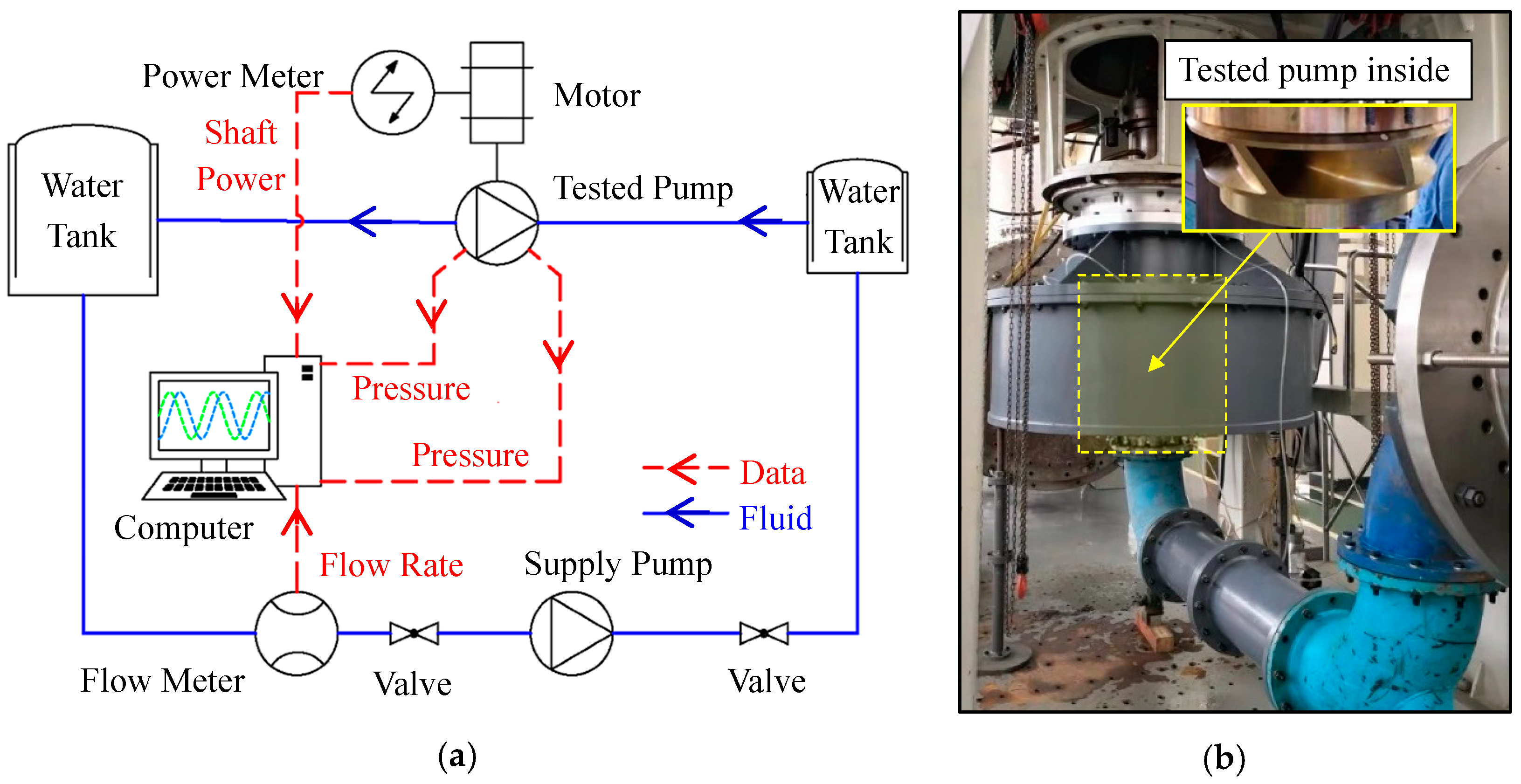
Figure 4 shows the model test rig used for numerical-experimental verification. The pump head and efficiency were verified to have a correct prediction of flow field in the pump. The pump head H was tested by acquiring the pressure difference between the inlet and outlet, and calculating. The flow rate Q was tested using the electromagnetic flow meter. The shaft power Psft was tested by the power meter, which acquired the rotating speed and torque, respectively. The efficiency η, including mechanical, volumetric, and hydraulic efficiencies, was calculated using the flow rate, shaft power, and head by η = ρgQH/Psft, where g is the acceleration of gravity.
4. Experimental Verification of Computation
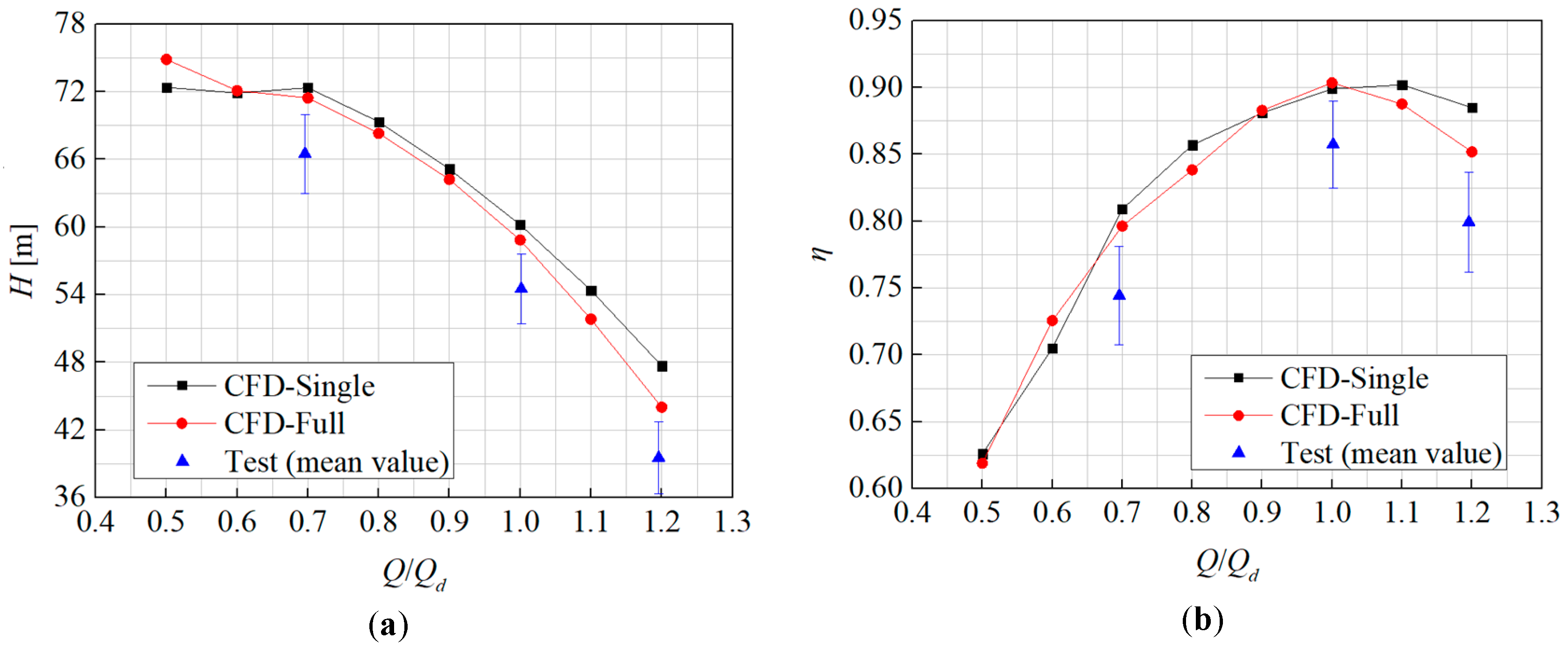
The pump performance, including head H and efficiency η, was used for the experimental verification of computation, as shown in Figure 5, before optimization design. “CFD-Full” refers to the CFD simulation calculated using the full passage of impeller and guide vanes. “CFD-Single” refers to the CFD simulation calculated using the single passages of impeller and guide vanes. Differences can be found between the single-passage result and the full-passage result. This is because of the simplification of the flow domain and the approximation of rotor-stator interface. However, the single-passage result, which was commonly seen in CFD simulations of turbomachinery [24,25], shows the same variation tendency under different conditions. Therefore, it can be accepted with full-passage verification after optimization. In this experiment, the pipelines and flow passages for connecting the impeller and guide vane were also considered. The mechanical and volumetric losses were considered in the experimental data. It was shown that the CFD values were slightly higher than the experimental value for both the head and efficiency. Generally, it can be observed that the CFD simulation captured the head and efficiency well when comparing with the experiment.
5. Results of Optimization Design
5.1. Optimization Process
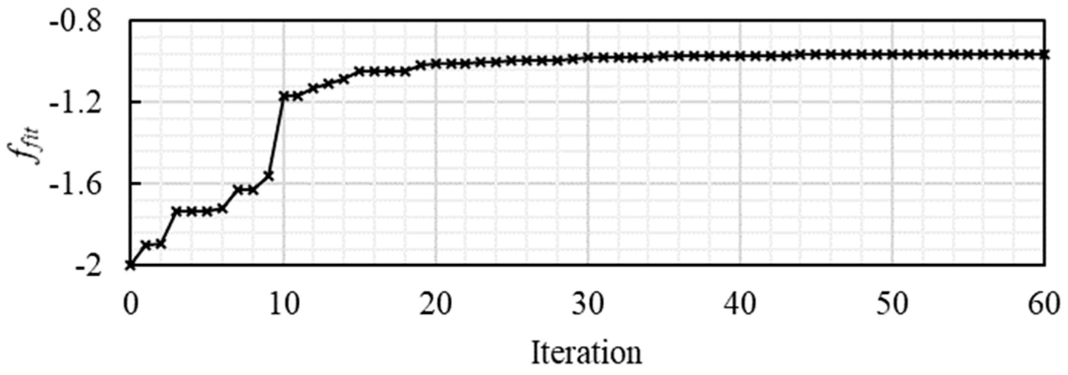
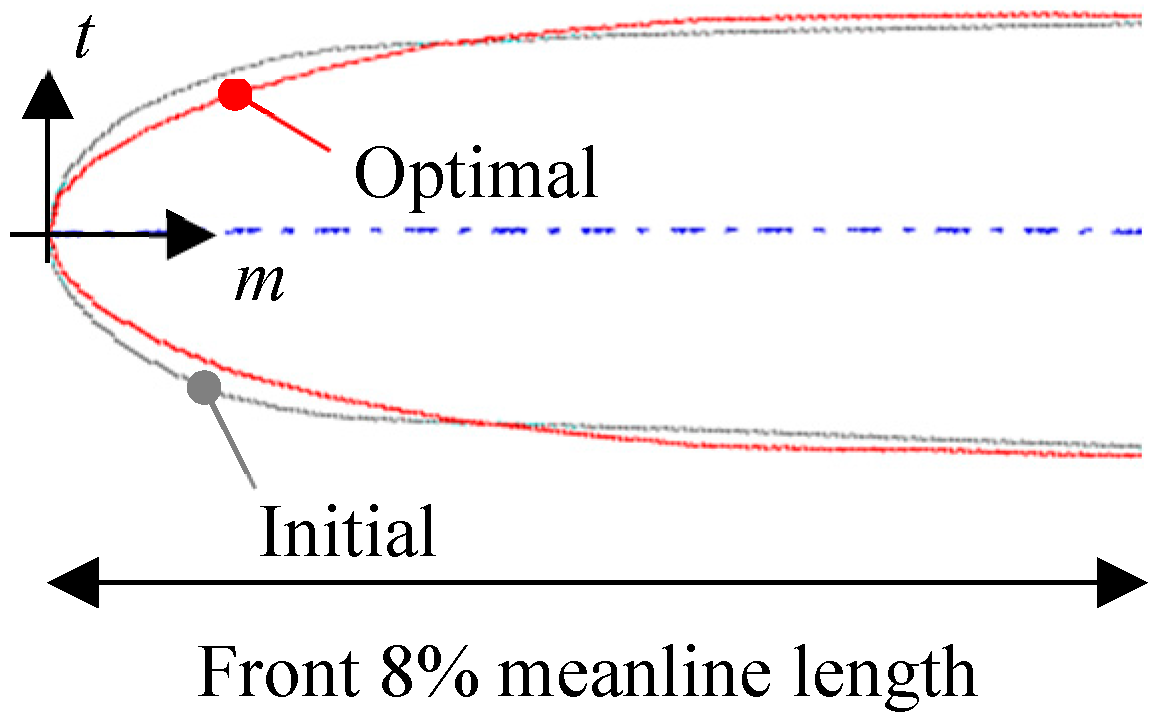
Figure 6 shows the optimization process of the ffit changing with iteration steps. The ffit value of the initial impeller sample was −1.9945. After 60 iterative steps of optimization, the ffit value increased to about −0.9615, and converged when the residual was continually less than 0.1% for 10 steps. The comparison of blade thickness around the leading-edge is shown in Figure 7. The design parameter Rab changed from 2.00 to 3.96, γs changed from 5.97° to 4.03°, and B changed from 1.50 to 3.00. The −Cpmin values varied from −3.06 to −1.025 at 0.7 Qd, from −1.19 to −1.363 at 1.0 Qd, and from −0.755 to −0.588 at 1.2 Qd. The main improvements were under the partial-load 0.7 Qd and the over-load 1.2 Qd. At the design load, the cavitation performance was somehow deteriorated.
5.2. Analysis of Cavitation Performance
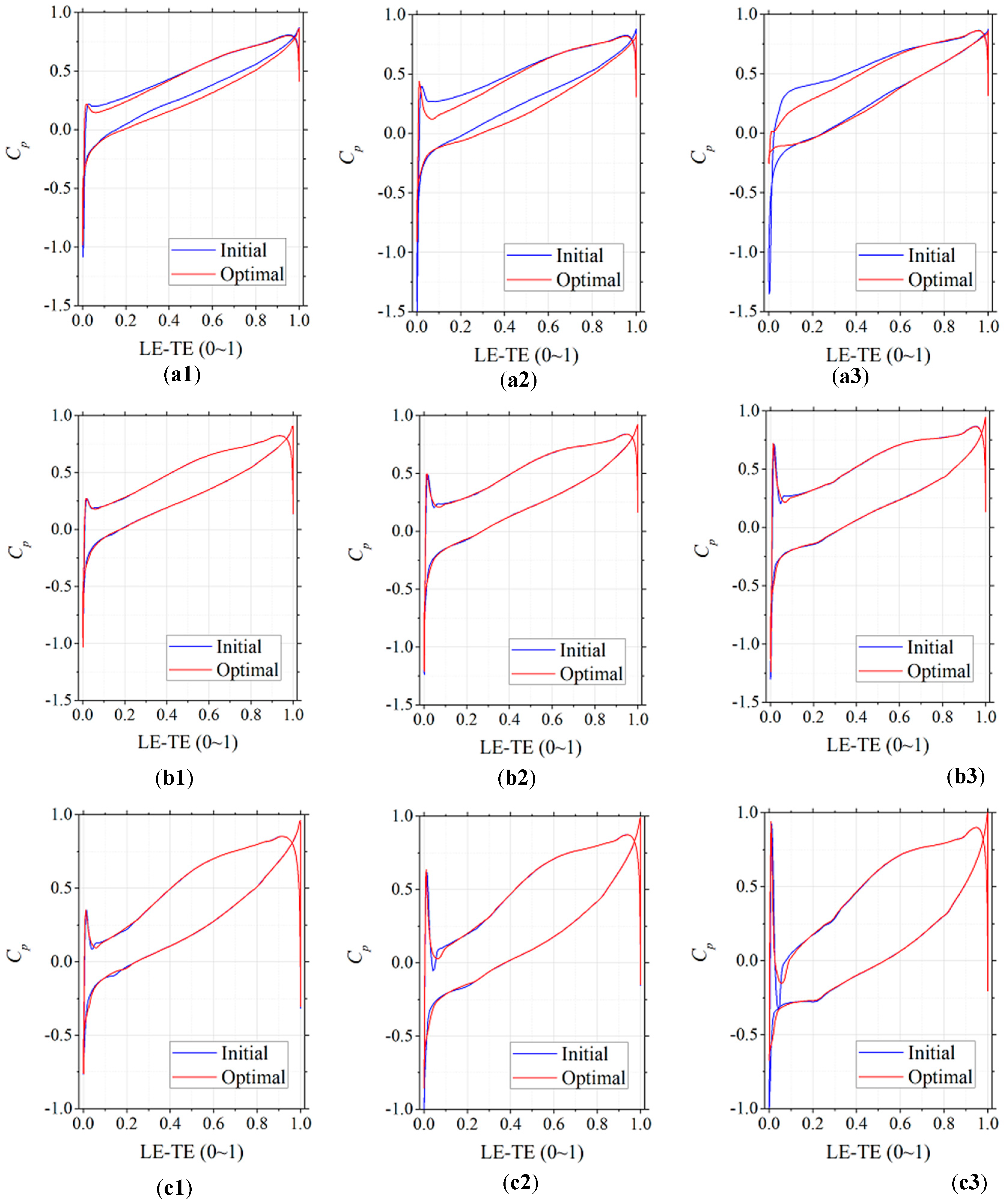
Figure 8 shows the Cp distributions on the initial and optimal impeller blades. Sudden pressure drops can be found on the blade leading-edge because of the local flow separation. After optimization, the leading-edge pressure drops became much gentler at 0.7 and 1.2 Qd, especially on the spanwise 0.9 surface (spanwise 0 is the hub and 1 is the shroud). At 0.7 Qd, a Cpmin value of about −1.5 occurred on the mid-span of the initial impeller. After optimization, the Cpmin value became about −1.0 near the hub. At 1.0 Qd, a Cpmin value of about −1.28 occurred near the shroud of the initial impeller. After optimization, the Cpmin value was still around −1.0 near the shroud without any improvement. At 1.2 Qd, a Cpmin value of about −1.0 occurred on the mid-span and near the shroud of the initial impeller. After optimization, the Cpmin value became about −0.8, which was located on the mid-span.
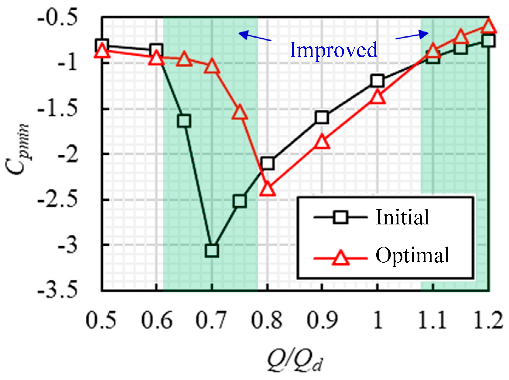
Figure 9 shows the Cpmin law at different flow rate conditions. Before optimization, the condition-minimum Cpmin value of about −3.06 was at 0.7 Qd. After optimization, the condition-minimum Cpmin value increased to about −2.37. Its flow rate condition became 0.8 Qd. The cavitation inception performance was improved in the two ranges of 0.62–0.78 Qd and 1.08–1.20 Qd, as illustrated in Figure 9. The head and efficiency changes were less than 0.5% after optimization in the 0.5–1.2 Qd flow rate range according to the single-passage CFD prediction.
5.3. Comparison of Head and Efficiency
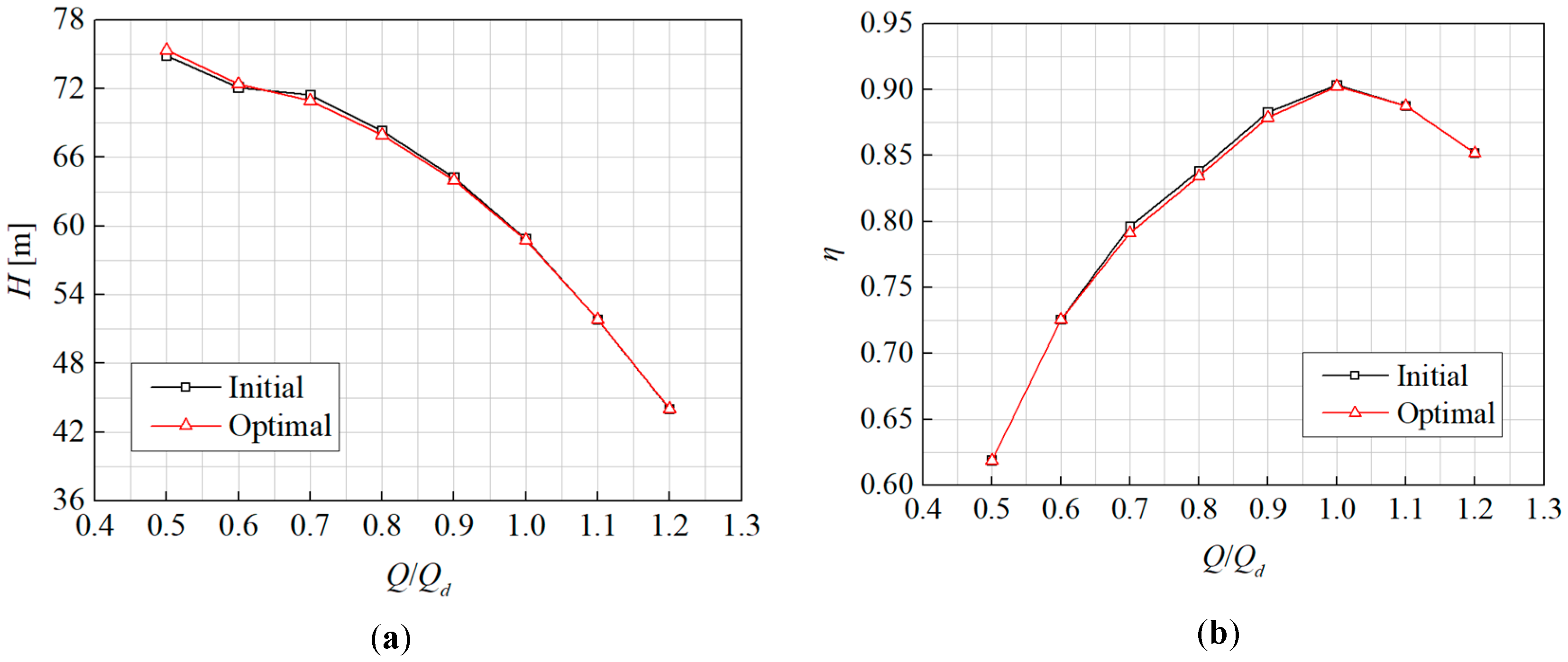
Figure 10 shows the comparisons of head and efficiency between the initial and optimal impeller. The influence of optimization on head and efficiency is small. Compared with the initial design, the maximum difference of the optimal head is 0.7%, and the maximum difference of the optimal efficiency is 0.6%. This shows that the optimization of blade leading-edge shape has little effect on head and efficiency. This meets the conclusion in IEC standards [26] that slight shape changes will not affect the hydraulic performance of hydro-turbomachinery.
6. Conclusions
In this study, the Diffusion-Angle Integral (DI) method, the Genetic Algorithm (GA), and the Computational Fluid Dynamics (CFD) method were used to optimize the cavitation performance of the mixed-flow pump impeller. The geometry (thickness distribution) around the leading-edge was redesigned. Conclusions can be drawn as follows:
(a) The DI method successfully reduced the design parameter number to three. The design time cost can be reduced by keeping the accurate shaping of the blade geometry. The rotating periodic boundaries were also used to simplify the CFD simulation. By giving the reasonable ranges of the design parameters, the optimization converged within just 60 iterations. The fitness function ffit increased from about −1.9945 to about −0.9615 after optimization design. The combination strategy used in this case provided a quick and reliable solution for the optimization of pump impellers.
(b) After optimization, the thickness t distribution along the mean line m obviously changed in law, and slightly changed in value. As a result, the cavitation performance was obviously improved, with only slight influences on head and efficiency. In detail, the condition-minimum Cpmin value strongly increased within the 0.5–1.2 Qd flow rate range, and the cavitation performance in the 0.62–0.78 Qd, and 1.08–1.20 Qd ranges was obviously improved.
The combination strategy or the individual methods used in this study were proven to be effective and can be applied to similar optimization design cases for other pump design cases.
Author Contributions
Investigation, D.Z.; methodology, R.T.; supervision, R.X.
Funding
National Natural Science Foundation of China: 51879265; National Natural Science Foundation of China: 51836010; China Postdoctoral Science Foundation: 2018M640126.
Acknowledgments
The authors would like to acknowledge the support of National Natural Science Foundation of China No. 51879265, National Natural Science Foundation of China No. 51836010 and China Postdoctoral Science Foundation No. 2018M640126.
Conflicts of Interest
The authors declare no conflicts of interest.
References
- Brennen, C.E. Cavitation and Bubble Dynamics; Oxford University Press: Oxford, UK, 1995. [Google Scholar]
- Franc, J.P.; Michel, J.M. Fundamentals of Cavitation; Springer: Dordrecht, The Netherlands, 2010. [Google Scholar]
- Wu, Q.; Huang, B.; Wang, G.; Cao, S.; Zhu, M. Numerical modelling of unsteady cavitation and induced noise around a marine propeller. Ocean Eng. 2018, 160, 143–155. [Google Scholar] [CrossRef]
- Valentín, D.; Presas, A.; Egusquiza, M.; Valero, C.; Egusquiza, E. Transmission of high frequency vibrations in rotating systems. Application to cavitation detection in hydraulic turbines. Appl. Sci. 2018, 8, 451. [Google Scholar] [CrossRef]
- Wu, S.; Zuo, Z.; Stone, H.A.; Liu, S. Motion of a Free-Settling Spherical Particle Driven by a Laser-Induced Bubble. Phys. Rev. Lett. 2017, 119, 084501. [Google Scholar] [CrossRef] [PubMed]
- Mouvanal, S.; Chatterjee, D.; Bakshi, S.; Burkhardt, A.; Mohr, V. Numerical prediction of potential cavitation erosion in fuel injectors. Int. J. Multiph. Flow 2018, 104, 113–124. [Google Scholar] [CrossRef]
- Pan, Z.; Yuan, S. Fundamentals of Cavitation in Pumps; Jiangsu University Press: Zhenjiang, China, 2013. [Google Scholar]
- Hao, Y.; Tan, L. Symmetrical and unsymmetrical tip clearances on cavitation performance and radial force of a mixed flow pump as turbine at pump mode. Renew. Energy 2018, 127, 368–376. [Google Scholar] [CrossRef]
- Hirschi, R.; Dupont, P.; Avellan, F.; Favre, J.N.; Guelich, J.F.; Parkinson, E. Centrifugal pump performance drop due to leading edge cavitation: Numerical predictions compared with model tests. J. Fluids Eng. Trans. ASME 1998, 120, 705–711. [Google Scholar] [CrossRef]
- Koukouvinis, P.; Gavaises, M.; Supponen, O.; Farhat, M. Simulation of bubble expansion and collapse in the vicinity of a free surface. Phys. Fluids 2016, 28, 052103. [Google Scholar] [CrossRef] [Green Version]
- Susan-Resiga, R.; Vu, T.C.; Muntean, S.; Ciocan, G.D.; Nennemann, B. Jet control of the draft tube vortex rope in Francis turbines at partial discharge. In Proceedings of the 23rd IAHR Symposium on Hydraulic Machinery and Systems, Yokohama, Japan, 17–21 October 2006. [Google Scholar]
- Yang, W.; Xiao, R.; Wang, F.; Wu, Y. Influence of splitter blades on the cavitation performance of a double suction centrifugal pump. Adv. Mech. Eng. 2014, 6, 963197. [Google Scholar] [CrossRef]
- Yao, Z.; Xiao, R.; Wang, F.; Yang, W. Numerical investigation of cavitation improvement for a francis turbine. In Proceedings of the 9th International Symposium on Cavitation, Lausanne, Switzerland, 6–10 December 2015. [Google Scholar]
- Liu, Y.; Li, Y.; Han, W.; Song, H.D.; Chen, J.X. Effect of geometric parameters of centrifugal pump inlet on its cavitation performance. J. Lanzhou Univ. Technol. 2011, 37, 50–53. [Google Scholar]
- Visser, F.C.; Dijkers, R.J.H.; Op De Woerd, J.G.H. Numerical flow-field analysis and design optimization of a high-energy first-stage centrifugal pump impeller. Comput. Vis. Sci. 2000, 3, 103–108. [Google Scholar] [CrossRef]
- Toyoda, M.; Nishida, M.; Maruyama, O.; Yamane, T.; Tsutsui, T.; Sankai, Y. Geometric optimization for non-thrombogenicity of a centrifugal blood pump through flow visualization. JSME Int. J. 2002, 45, 1013–1019. [Google Scholar] [CrossRef]
- Liu, H.; Wang, K.; Yuan, S.; Tan, M.; Wang, Y.; Dong, L. Multicondition optimization and experimental measurements of a double-blade centrifugal pump impeller. J. Fluids Eng. 2013, 135, 111031. [Google Scholar] [CrossRef] [PubMed]
- Tao, R.; Xiao, R.; Wang, F.; Liu, W. Cavitation behavior study in the pump mode of a reversible pump-turbine. Renew. Energy 2018, 125, 655–667. [Google Scholar] [CrossRef]
- Tao, R.; Xiao, R.; Wang, Z. Influence of blade leading-edge shape on cavitation in a centrifugal pump impeller. Energies 2018, 11, 2588. [Google Scholar] [CrossRef]
- Tao, R.; Xiao, R.; Wang, F.; Liu, W. Improving the cavitation inception performance of a reversible pump-turbine in pump mode by blade profile redesign: Design concept, method and applications. Renew. Energy 2019, 133, 325–342. [Google Scholar] [CrossRef]
- Xuan, G. Genetic Algorithms and Engineering Optimization; Tsinghua University Press: Beijing, China, 2004. [Google Scholar]
- Menter, F.R. Ten years of experience with the SST turbulence model. Turbul. Heat Mass Transf. 2003, 4, 625–632. [Google Scholar]
- Spalart, P.R. Detached-Eddy Simulation. Annu. Rev. Fluid Mech. 2009, 41, 203–229. [Google Scholar] [CrossRef]
- Zhong, L.; Lai, X.; Liao, G.; Zhang, X. Analysis on the relationship between swirling flow at outlet of a Francis turbine runner and vortex rope inside draft tube. J. Hydroelectr. Eng. 2018, 37, 40–46. [Google Scholar]
- Tao, R.; Xiao, R.; Yang, W.; Wang, F.; Liu, W. Optimization for cavitation inception performance of pump-turbine in pump mode based on genetic algorithm. Math. Probl. Eng. 2014, 2014, 234615. [Google Scholar] [CrossRef]
- International Electrotechnical Commission. Hydraulic Turbines, Storage Pumps and Pump-Turbines-Model Acceptance Tests, 2nd ed.; International Standard IEC 60193; IEC: Geneva, Switzerland, 1999. [Google Scholar]
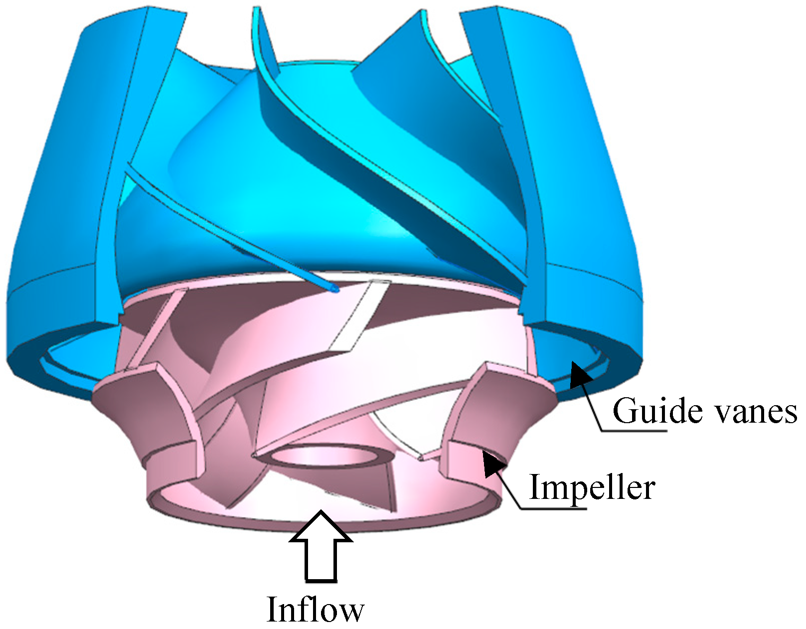
Figure 1.
Schematic map of the mixed-flow pump.

Figure 2.
Parameter control. (a) Traditional parameter control; (b) Diffusion-Angle Integral (DI) method.
Figure 2.
Parameter control. (a) Traditional parameter control; (b) Diffusion-Angle Integral (DI) method.

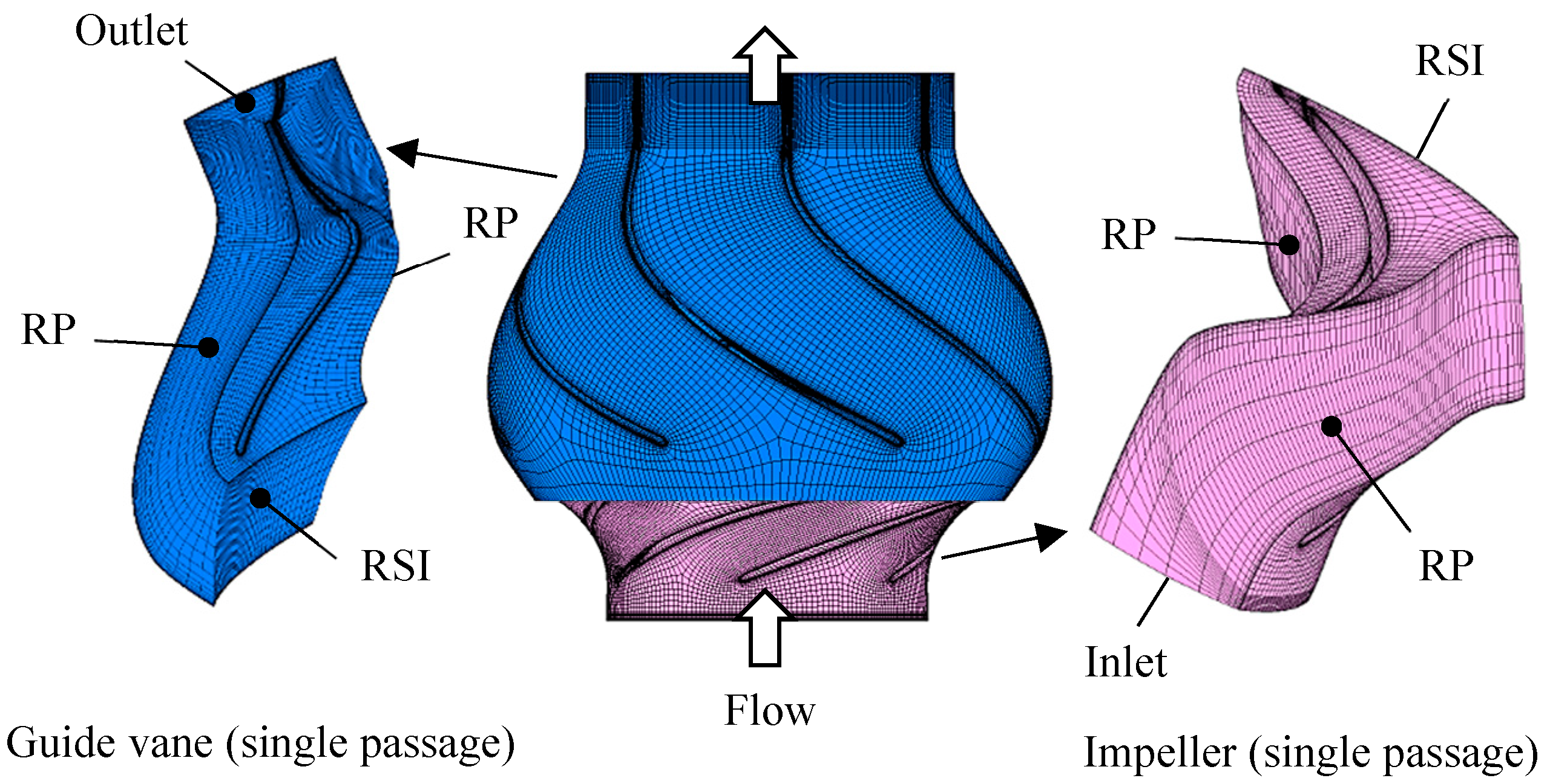
Figure 3.
Schematic map of the flow domain, mesh, and boundaries. RP is the rotational periodic boundary, RSI is the rotor-stator interface, and other unmarked boundaries are no slip walls.
Figure 3.
Schematic map of the flow domain, mesh, and boundaries. RP is the rotational periodic boundary, RSI is the rotor-stator interface, and other unmarked boundaries are no slip walls.

Figure 4.
The pump model test rig. (a) Schematic map of test rig; (b) Test rig on site.

Figure 5.
The experimental and Computational Fluid Dynamics (CFD)-predicted data of head and efficiency before optimization. (a) Head curves; (b) Efficiency curves.
Figure 5.
The experimental and Computational Fluid Dynamics (CFD)-predicted data of head and efficiency before optimization. (a) Head curves; (b) Efficiency curves.

Figure 6.
The monitoring of the optimization process.

Figure 7.
Thickness comparison.

Figure 8.
Cp distributions on initial and optimal impeller blades. (a1) 0.7 Qd, Spanwise 0.1; (a2) 0.7 Qd, Spanwise 0.5; (a3) 0.7 Qd, Spanwise 0.9; (b1) 1.0 Qd, Spanwise 0.1; (b2) 1.0 Qd, Spanwise 0.5; (b3) 1.0 Qd, Spanwise 0.9; (c1) 1.2 Qd, Spanwise 0.1; (c2) 1.2 Qd, Spanwise 0.5; (c3) 1.2 Qd, Spanwise 0.9

Figure 9.
Condition-minimum Cpmin values from 0.5 to 1.2 Qd.

Figure 10.
The comparisons of head and efficiency between the initial and optimal impeller blades. (a) Head; (b) Efficiency.
Figure 10.
The comparisons of head and efficiency between the initial and optimal impeller blades. (a) Head; (b) Efficiency.


Table 1.
Design and operation parameters of the pump.
| Parameter | Value |
|---|---|
| Rotation speed nd | 1470 [rpm] |
| Design flow rate Qd | 1 [m3/s] |
| Design head Hd | 55 [m] |
| Specific speed nq | 72.8 |
| Impeller blade number | 6 |
| Guide vane blade number | 7 |
| Impeller inlet diameter D1 | 0.4 [m] |
Table 2.
Probabilities of genetic operations.
| Operation | Copy/Eliminate | Crossover | Mutation |
|---|---|---|---|
| Probability | 1.0 | 0.6 | 0.1 |
Table 3.
Parameter range in optimization.
| Parameter | Rab | γs [°] | B |
|---|---|---|---|
| Range | 1–5 | 1–10 | 1–6 |
Table 4.
Mesh independence check.
| Number of Mesh Nodes [×106] | 0.3180 | 0.5594 | 0.8269 | 1.2056 | 1.7427 | 2.3546 |
| Residual [%] | 100 | 1.1862 | 0.7266 | 0.0809 | 0.3019 | 0.3782 |
© 2019 by the authors. Licensee MDPI, Basel, Switzerland. This article is an open access article distributed under the terms and conditions of the Creative Commons Attribution (CC BY) license (http://creativecommons.org/licenses/by/4.0/).
Share and Cite
MDPI and ACS Style
Zhu, D.; Tao, R.; Xiao, R. Anti-Cavitation Design of the Symmetric Leading-Edge Shape of Mixed-Flow Pump Impeller Blades. Symmetry 2019, 11, 46. https://doi.org/10.3390/sym11010046
AMA Style
Zhu D, Tao R, Xiao R. Anti-Cavitation Design of the Symmetric Leading-Edge Shape of Mixed-Flow Pump Impeller Blades. Symmetry. 2019; 11(1):46. https://doi.org/10.3390/sym11010046
Chicago/Turabian StyleZhu, Di, Ran Tao, and Ruofu Xiao. 2019. "Anti-Cavitation Design of the Symmetric Leading-Edge Shape of Mixed-Flow Pump Impeller Blades" Symmetry 11, no. 1: 46. https://doi.org/10.3390/sym11010046
Note that from the first issue of 2016, this journal uses article numbers instead of page numbers. See further details here.