Modeling the Service Network Design Problem in Railway Express Shipment Delivery


School of Traffic and Transportation, Beijing Jiaotong University, Beijing 100044, China
*
Author to whom correspondence should be addressed.
Symmetry 2018, 10(9), 391; https://doi.org/10.3390/sym10090391
Submission received: 22 August 2018
/
Revised: 30 August 2018
/
Accepted: 2 September 2018
/
Published: 10 September 2018
(This article belongs to the Special Issue Symmetry in Engineering Sciences)
Abstract
:As air pollution becomes increasingly severe, express trains play a more important role in shifting road freight and reducing carbon emissions. Thus, the design of railway express shipment service networks has become a key issue, which needs to be addressed urgently both in theory and practice. The railway express shipment service network design problem (RESSNDP) not only involves the selection of train services and determination of service frequency, but it is also associated with shipment routing, which can be viewed as a service network design problem (SNDP) with railway characteristics. This paper proposes a non-linear integer programming model (INLP) which aims at finding a service network and shipment routing plan with minimum cost while satisfying the transportation time constraints of shipments, carrying capacity constraints of train services, flow conservation constraint and logical constraints among decision variables. In addition, a linearization technique was adopted to transform our model into a linear one to obtain a global optimal solution. To evaluate the effectiveness and efficiency of our approach, a small trial problem was solved by the state-of-the-art mathematical programming solver Gurobi 7.5.2.
1. Introduction
In recent years, air pollution has become a severe problem which has to be solved urgently across the world. Many countries have endeavored to reduce carbon emissions related to the transportation industry, which is one of the main sources of air pollution. As the average carbon emissions per workload of road transport is 3.36 to 4.64 times higher than that of railway transport [1], diverting road freight to rail is a wise option. In Europe, 30% of road freight over 300 km should shift to other modes such as rail or waterborne transport by 2030, and more than 50% by 2050 [2]. The Ministry of Transport of China also recommends that the railways and waterways should support more freight transportation. Since the shipments carried by road are generally high-value commodities, which are sensitive to delivery time instead of transportation cost, the express train, which features fast speed, guaranteed pickup and delivery time, plays an increasingly important role in competing with trucks and reducing carbon emissions. The railway express shipment service network design problem express shipment service network design problem (RESSNDP) can be viewed as a service network design problem service network design problem (SNDP) with characteristics of the railway industry. It not only involves the construction of service networks (selection of train services and determination of service frequency), but is also associated with the routing of shipments. Additionally, there is a trade-off between service quality (i.e., transportation capacity and delivery time) and total cost (including service providing cost, shipment routing cost and time cost). Theoretically, the combinations of train services grow exponentially with the number of stations, train speed levels, and stop strategies. Furthermore, each service network involves shipment routing problems which are also exponential explosion problems. Therefore, the RESSNDP has become a key issue that needs to be addressed both in theory and practice.
The problems that arise in railway transportation can be grouped into three levels: the strategic level, tactical level and operational level. Problems at the strategic level are characterized by lengthy time horizons and typically involve resource acquisition. Tactical level problems focus more on allocating resources across an infrastructure that is assumed to be fixed. Operational problems are defined as those that occur on a day-to-day basis. As the RESSNDP is involved with the allocation of express trains over the physical network, it is a tactical level problem, i.e., specific arrival/departure time of trains is not considered in this study.
The paper is organized as follows: Section 1 introduces the importance and complexity of the RESSNDP. Section 2 provides a brief survey of the literature devoted to the SNDP. In Section 3, we describe the RESSNDP in detail. In Section 4, we establish a non-linear integer programming model and transform it into a linear one by applying linearization techniques. A small-scale trial study is conducted in Section 5, and conclusions are presented in Section 6.
2. Literature Review
The RESSNDP can be abstracted as a SNDP, which is a classical problem in the field of traffic and transportation that many scholars have researched. Several studies that are closely related to the SNDP in the railway industry should be noted. A classical paper is that of Crainic et al. [3] who presented a general optimization model which took into account the interactions between routing freight traffic, scheduling train services and allocating classification work on a rail network. Barnhart et al. [4] formulated railroad blocking problems as a mixed integer programming (MIP) model with maximum degree and flow constraints on the nodes and proposed a heuristic Lagrangian relaxation approach to solve the problem. Campetella et al. [5] considered a SNDP in the Italian rail system, and proposed a model combining full and empty railcar management, service selection and frequency. Ahuja et al. [6] proposed a particularly detailed model for a railroad blocking problem arising in the United States and developed an algorithm using the very large-scale neighborhood search technique. Lin et al. [7] presented a formulation and solution for the train connection service problem in a Chinese railway network to determine the optimal freight train service, the frequency of service, and the distribution of classification workload among yards. Zhu et al. [8] addressed the scheduled service network design problem by proposing a model that integrated service selection and scheduling, car classification and blocking, train make-up, and the routing of time-dependent customer shipments based on a cyclic three-layer space-time network representation of the associated operations and decisions, and their relations and time dimensions. The literature mentioned above is mainly devoted to the selection and scheduling of services, as well as routing of shipments. In addition, a variety of techniques, such as Lagrangian relaxation, very large-scale neighborhood search, simulated annealing, etc., have been implemented to solve realistically-size problems.
There is a rich body of literature on express shipment SNDP. Barnhart and her research team [9,10] proposed a column generation-based method to address a real-life air cargo express delivery SNDP. However, it might be difficult to generalize the model to other freight transportation applications, especially to those without hub-and-spoke structures. Grunert et al. [11] and Smilowitz et al. [12] studied long-haul transportation in postal and package delivery systems, and established several models and solution approaches. Armacost et al. [13] proposed an approach for solving express shipment SNDPs by introducing composite variables, which were the combinations of aircraft routes, implicitly capturing package flows. Wang et al. [14] studied a dynamic SNDP for express shipment delivery and established a mixed integer programming model of multi-modal transportation. Yu et al. [15] constructed a bi-level model to optimize the flight transportation network of an express company. The upper-level program was aimed at designing the network and allocating the transportation capacity, and the lower-level program was intended to calculate the link flows in user equilibrium. Quesada et al. [16] developed a formulation in which the allocation of packages to hubs was a decision variable of the model. Also, the formulation was strengthened with three families of valid inequalities and the forcing constraints were reformulated for reducing the number of variables and constraints. Zhao et al. [17] built a hybrid hub-spoke express network decision model permitting direct shipment delivery, whose objective was to minimize the total transport costs of the network. Wang and He [18] investigated the resource planning optimization problem for the multi-modal express shipment network, and a multi-stage hybrid genetic algorithm was presented to solve the model. To our knowledge, the studies on RESSNDP started relatively late and there is limited related literature. Ceselli et al. [19] established three models, integer linear programming (ILP) models, for the express service network of Swiss federal railways using different methods, and designed corresponding solution methods that included a commercial solver approach, branch-and-cut approach, and column generation-based approach. A comparison between a few published studies on SNDP and this work is presented in Table 1.
As shown in Table 1, a majority of the models proposed in the abovementioned studies are integer/mixed-integer programming models, which are difficult to solve to optimality. Thus, a variety of heuristic algorithms are adopted to solve them. In addition, as much of the literature focuses on the railway SNDP of bulk cargo, transportation time and speed levels of freight trains are not considered. In fact, due to the high added-value of express shipments, cargo owners generally pay more attention to the transportation time instead of freight rate, and carriers usually provide express trains on different speed levels to meet the demands of cargo owners. Furthermore, as an express train might stop at a certain number of intermediate stations on its itinerary for the attachment/detachment of blocks (the railcars carrying the same shipment are defined as a block, which does not split until arrival at the destination), the stop strategy plays an important role in the construction of express service network. Thus, we are motivated to carry out this study, and the contribution of our study is as follows:
Firstly, a non-linear integer programming model is proposed which not only takes into account the constraints of transportation time, service capacity, and flow conservation, but also considers the speed levels and stop strategies of train services, the block attachment/detachment operations in intermediate stations, as well as the time cost of express shipments. Secondly, linearization techniques are employed to transform our model into a linear one, in order to obtain a global optimal solution. Thirdly, a small-scale trial study is conducted and a state-of-the-art commercial software Gurobi is adopted to solve our model.
3. Problem Description
The RESSNDP can be viewed as a SNDP with characteristics of the railway industry. It is not only involved with the construction of service network, but is also associated with the routing of shipments. To facilitate the description of the RESSNDP, we constructed a service network as depicted in Figure 1.
As shown in Figure 1, there are 10 train services (TS01 to TS10), including six services at speed level I (denoted by the solid line, 80 km/h), two services at speed level II (dashed line, 120 km/h), and two services at speed level III (dot-dashed line, 160 km/h). The frequency (i.e., the number of trains dispatched per day) of TS03 and TS08 is two and three, respectively, while the frequency of other train services is set to one. Note that, TS01, TS02, TS03, TS06 and TS08 will stop (denoted by a hexagon) at station S2, S3, S4, S4 and S3, respectively, for block attachment/detachment. Dispatching a train will incur a fixed cost and a variable cost which is involved with operation mileage. For example, the cost of providing service TS01 can be calculated by , where is the fixed cost of dispatching an express train at speed level I, is the transportation cost per kilometer of an express train at speed level I, is the distance between S1 and S3, and “1” is the number of trains dispatched from S1 to S3. Similarly, the cost of providing service TS02 can be calculated by .
The second step is to assign the shipments to the service network we constructed. For example, if the shipment which originates at S1 and is destined to S5 is carried by TS02, it will be first sent to station S2, then stop at S2 for a couple of hours (about two hours in practice, mostly due to the attachment/detachment of other blocks, partly because of routine inspection), and finally delivered to the destination S5. The routing cost of this shipment (S1, S5) can be calculated by:
where is the transportation cost of a loaded railcar per kilometer when carried by a train at speed level III, is the railcar volume of shipment (S1, S5), is the waiting cost (including the expense of labor in inspecting the cargo damage and evaluating the performance of the train, and fuel consumption in the arrival and departure process at the intermediate station) of a railcar in average at station S3. In fact, as high-value commodities are very sensitive to the transportation time, it is necessary to take into account the time cost of shipments. In this case, the time cost of shipment (S1, S5) can be expressed by:
where is the coefficient of converting car-hour cost into economic cost, is the travel speed of train at level III, is the average waiting time of a railcar at station S3. Therefore, the sum of routing cost and time cost of shipment (S1, S5) is equal to:
In this way, the transport cost and waiting cost at S3 of a railcar can be generalized by and , respectively, which are defined as follows:
Similarly, if the shipment (S1, S5) is transport by TS01 and TS03, it will be first carried by TS01 from station S1 to station S2, then transferred (detached from a train and attached to another) to TS03 at S2, and finally sent to the destination S5 after a stop at S4. It should be noted that transferring at a station might take about six hours. Throughout the whole process, the generalized routing cost (including routing cost and time cost) of the shipment will be:
where is the generalized transfer cost at station S2, which can be expressed by:
In fact, the combinations for constructing a service network grows exponentially with the number of stations, speed levels, and stop strategies. So, there are a huge number of combinations even in a small railway network. For instance, if there are three optional speed levels for each potential train service and the train might stop at a certain number of intermediate stations it passes through, the combinations of service network construction will be 64 () for two stations, 2,985,984 () for three stations and over 2.1 quadrillion () for four stations. Furthermore, each service network is involved with a shipment routing problem which is also an exponential explosion problem. Thus, the RESSNDP is of huge complexity.
4. Mathematical Model
In this section, we first describe the assumptions proposed for our study, then introduce the notations used in this paper in Section 4.1, followed by model formulations (see Section 4.2), and finally, we adopt linearization techniques to linearize our model in Section 4.3.
Assumption 1.
Each shipment cannot be split until arriving at the destination. In other words, each shipment can only be delivered along one physical path, and can only choose one service chain (a sequence of train services). Although splitting a shipment and assigning the commodities to different paths and service chains might reduce the total operation cost, the no splitting rule is widely adopted by railway departments in practice for its simplicity in operations management.
Assumption 2.
It is assumed that the physical path of each origin-destination (OD) demand (i.e., shipment) is specified in advance, which is a standard practice used in the Chinese railway system in freight transportation. As it might result in higher operational costs compared with joint optimization of the railcar itinerary and shipment delivery strategy, one solution to this problem is to optimize train paths and railcar reclassification plans simultaneously.
Assumption 3.
For each potential train service, only one stop strategy can be selected. For example, for the OD pair , only one stop strategy can be selected for the express trains (at the same speed level, such as 80km/h) dispatched from to . It simplifies the problem to some extent by excluding a lot of optional stop strategies once a strategy is chosen.
4.1. Notations
The notations used in this paper are listed in Table 2.
4.2. Formulations
In the delivery of express cargo, there are different types of cost that should be taken into consideration. The generalized transport cost (including transport cost and time cost) involved with the volume of loaded railcar and operation mileage can be expressed by:
As a block might be detached from one train and attached to another on its itinerary, the generalized block transfer cost should be considered. It can be expressed by:
Note that, block transfer will occur when the shipment is delivered by at least two trains with different origins, destinations or speed levels.
When a train stops at a certain station, the block that does not need to be transferred here may incur waiting cost, due to attachment/detachment of other blocks, routine inspection of cargo damage, train performance evaluation and other transit operations. The generalized waiting cost can be calculated as:
In this paper, we define the sum of the generalized transport cost, transfer cost and waiting cost as the generalized shipment routing cost. In addition, when a train service is provided, a service providing cost will be incurred, consisting of a fixed cost associated with speed level and a variable cost involved with operation mileage, which can be expressed by:
For an express train dispatched from to , the set of its stop strategy is denoted as . Among them, a special strategy should be noted, i.e., . In this case, the express train will not stop at any station on its itinerary, including to . In other words, no service from to will be provided. Conversely, if an express train stops at every station it passes through on its itinerary, then the stop strategy might be . The set of decision variables for a potential service on speed level can be denoted as:
According to Assumption 3, the following constraint should be considered:
Therefore, the RESSNDP can be formulated as a non-linear integer programming model whose objective function and constraints are written as follows:
The objective function is to minimize the sum of the service providing cost, shipment routing cost and time cost. The constraint (15) ensures that, for each OD pair , only one stop strategy can be selected for the train service provided from to at speed level , . The constraint (16) is the flow conservation constraint which guarantees that all shipments can be delivered to their destination. The constraint (17) is the transportation time constraint which ensures that the sum of transport time, transfer time and waiting time of a shipment is less than the pre-specified due time. The constraint (18) is the capacity constraint which guarantees that the workload of a certain service arc is less than its carrying capacity, where is the size of the train. The constraint (19) is the logical constraint for the service selection variable and shipment routing variable, which ensures that the service arc would not be selected if it does not exist when stop strategy is chosen for the train service. The constraints (20) and (21) together guarantee that a shipment will be assigned to the service whose origin and destination are the same as that of the shipment, if the train service is provided. In other words, if there is no shipment whose origin and destination are the same as that of a candidate train service, the service will not be provided. The constraints (22) and (23) are the logical constraints for the service selection variable and service frequency variable, which indicate that at least one train will be provided when a stop strategy (excluding the non-stop strategy, i.e., ) is chosen. It should be noted that no train will be dispatched if stop strategy “0” is selected.
4.3. Linearization of the Model
As the INLP model is very difficult to be solved to optimality, linearization techniques are adopted to linearize the model we proposed. Apparently, the objective function (14), (17) and (21) have nonlinear terms, i.e., the product of binary variables: and . To solve it, we first introduced the method of linearizing the product of a sequence of binary variables. Let us assume that , where are all binary variables. Then can be equivalently expressed by the following linear inequality:
According to the formula , it is clear that is a binary variable. and when all take the value of one, is obviously equal to one. In contrast, if at least one variable of takes the value of zero, then is equal to zero. Similarly, on the basis of formula (26), when all take the value of one, this inequality can be rewritten as , i.e., . Thus, has to take the value of one. Conversely, if not all variables of take the value of one, i.e., , then the formula (26) can be converted to , i.e., . Thus, has to take the value of zero. To summarize, inequality (26) is equivalent to the equation . Based on the method mentioned above, the transfer variable and waiting variable are introduced, which can be expressed by:
The transfer variable takes the value of one if the shipment is detached from a train and attached to another at station . Otherwise, it is zero. Similarly, the waiting variable is equal to one if the shipment is carried by the same train before and after the stop at a certain intermediate station . Otherwise, it is zero. Moreover, several constraints should be added to the original model:
In this way, the original non-linear model can be converted to a linear one which can be expressed by:
s.t. Constraints (15) to (25) and (29) to (34). Thus, we can directly use a standard optimization solver to solve the model.
5. Numerical Study
In this section, we carried out a small-scale trial study to evaluate the effectiveness and validity of our model and approach. The procedures are described in detail as follows: (1) A physical railway network consisting of five stations, denoted as S1 through S5, was constructed which is depicted by Figure 2. (2) The OD matrix, transportation time constraint of each shipment, mileage of each OD pair, transfer cost, transfer delay, waiting cost and waiting delay at each station were determined and are listed in Table 3. (3) A commercial software, Gurobi 7.5.2, was adopted to solve the model. (4) We obtained the stop strategy and frequency of express trains which are to be provided, as well as the service chain (the sequence of express trains carrying a certain shipment) of each shipment. (5) To evaluate the impact of some critical parameters on the total cost and number of trains dispatched, sensitivity analysis was carried out.
According to the operational practices of express trains in China, the travel speed of trains at three speed levels (I, II, III) were set to 80 km/h, 120 km/h and 160 km/h respectively. The fixed cost of dispatching an express train at three speed levels were set to 5000 CNY, 6000 CNY and 7000 CNY, respectively, while the variable cost of an express train at three speed levels per kilometer were set to 40 CNY/km, 50 CNY/km and 60 CNY/km, respectively. In addition, the unit transportation cost of a railcar at three speed levels were set to 5 CNY/km, 6 CNY/km and 7 CNY/km respectively. Moreover, the train size was set to 25 cars.
The RESSNDP mentioned above was solved by Gurobi 7.5.2 on a 2.20 GHz Intel (R) Core (TM) i5-5200U CPU computer with 4.0 GB of RAM. After about 51 seconds of computation, the optimal solution was obtained. The total cost is 1,200,561.5 CNY (where the total service providing cost is equal to 435,690 CNY, the total generalized transport cost is 764,098.1 CNY, the total generalized transfer cost is equal to 433.8 CNY, the total generalized waiting cost is 339.6 CNY), and ten train services are supposed to be provided to carry the shipments in the network, including seven services at speed level I, two services at speed level II and one service at speed level III. The express services provided and their frequency are listed in Table 4 and the optimal service network is depicted by Figure 3.
It should be noted that the shipment (S1, S5) will transfer from train service TS01 to TS08 at the intermediate station S2; the shipment (S4, S3) will transfer from train service TS08 to train service TS10 at the intermediate station S2; the shipment (S5, S1) will transfer from train service TS10 to train service TS07 at the intermediate station S2; and the shipment (S5, S4) will transfer from train service TS10 to train service TS02 at the intermediate station S2. Furthermore, the shipments (S1, S3), (S1, S4), (S3, S5), (S4, S1), (S4, S5), (S5, S3) will all wait at station S2 for a couple of hours.
Sensitivity analysis was carried out to evaluate the impact of some critical parameters on total cost and number of trains dispatched, including the fixed cost and variable cost of dispatching an express train at a speed level of I, i.e., and ; the generalized transportation cost of a loaded railcar at a speed level of I per kilometer, i.e., ; train size . The standard value of these parameters and their step size are listed in Table 5.
As the result might be influenced by some or all parameters mentioned above, we only changed the value of one parameter each time and set the value of other parameters to their standard value, in order to evaluate their individual impact. The results are illustrated in Figure 4.
The impact of , , and on the total cost and number of trains dispatched are depicted by Figure 4a–d respectively.
As shown in Figure 4a, with the increase of , the total cost steadily grows from 1,190,062 CNY to 1,211,062 CNY, while the number of trains stays the same, i.e., ten trains are dispatched each day no matter how the fixed cost of dispatching an express train at speed level I changes. It is demonstrated that is positively correlated with the total cost while it has no impact on the number of trains dispatched.
Similarly, as shown in Figure 4b, as increases from 25 to 55, the total cost grows steadily from 1,110,727 CNY to 1,290,397 CNY while the number of trains dispatched remains stable no matter how the variable cost changes. It seems that the total cost increases with while the variable cost has no impact on the number of trains dispatched.
It can be seen from Figure 4c that the total cost grows with . On the contrary, the number of trains dispatched first remains unchanged when increases from 3.5 to 6, then decreases to nine trains when reaches 6.5. Thus, there is a negative correlation between the number of trains dispatched and .
From Figure 4d, we can see that both the total cost and number of trains are negatively correlated with the train size. When increases from 15 to 45, the total cost decreases from 1,379,512 CNY to 1,059,998 CNY, and the number of trains dispatched drops from 15 trains to five trains, respectively. This is because a train with larger size can accommodate more railcars at the same time, i.e., less train is needed to deliver the given shipments.
6. Conclusions
In this paper, we formulated the express train service network design problem as a non-linear integer programming model which aims at finding a service network and shipment routing plan with minimum cost, while satisfying the transportation time constraints of shipments, carrying capacity constraints of train services, the flow conservation constraint and logical constraints among decision variables. Moreover, the model takes into account the speed levels and stop strategies of express trains, the block attachment/detachment operations in intermediate stations, as well as the time cost of express shipments. In order to obtain a global optimal solution, a linearization technique was adopted to transform our model into a linear one, which can be solved to optimality by using commercial software in small-scale cases. To evaluate the effectiveness and efficiency of our approach, the state-of-the-art mathematical programming solver Gurobi 7.5.2 was adopted to solve our model and an optimal solution was obtained rapidly. Furthermore, sensitivity analysis was carried out for several critical parameters to evaluate their impact on the total cost and number of trains dispatched. Currently, the express train service plan is made by a team of highly-experienced service designers, i.e., it requires painstaking manual effort. In this case, the model and solution approach we proposed can be used as an aid for railway operators in making express train service plans or improving their current train schedules, hence, achieving substantial savings in capital costs by running far fewer trains and significantly reducing block swaps (the transfer of a block from one train to another is called a block swap). In the long term, researchers can focus on the optimization of specific arrival/departure times of express trains when solving the RESSNDP. Moreover, the development of an exact solution approach for large-scale problems is also promising for future research.
Author Contributions
The authors contributed equally to this work.
Acknowledgments
This work was supported by the National Natural Science Foundation of China (Grant no. 51378056), and the science technology and legal department of the National Railway Administration of the People’s Republic of China under Grant Number, KF2017-015.
Conflicts of Interest
The authors declare no conflict of interest.
References
- Lin, B.L.; Liu, C.; Wang, J.X.; Liu, S.Q.; Wu, J.P.; Li, J. Modeling the railway network design problem: A novel approach to considering carbon emissions reduction. Transp. Res. Part D Transp. Environ. 2017, 56, 95–109. [Google Scholar] [CrossRef]
- European Commission. Roadmap to a Single European Transport Area—Towards a Competitive and Resource Efficient Transport System; White Paper; European Commission: Brussels, Belgium, 2011; pp. 1–31. [Google Scholar]
- Crainic, T.G.; Kim, K.H. Transportation: Handbooks in Operations Research and Management Science; Barnhart, C., Laporte, G., Eds.; Elsevier: Amsterdam, The Netherlands, 2006; Volume 14, pp. 189–284. [Google Scholar]
- Barnhart, C.; Jin, H.; Vance, P. Railroad blocking: A network design application. Oper. Res. 2000, 48, 603–614. [Google Scholar] [CrossRef]
- Campetella, M.; Lulli, G.; Pietropaoli, U.; Ricciardi, N. Freight service design for the Italian railways company. In Proceedings of the ATMOS 6th Workshop on Algorithmic Methods and Models for Optimization Railways, Zurich, Switzerland, 14 September 2006. [Google Scholar]
- Ahuja, R.K.; Jha, K.C.; Liu, J. Solving real-life railroad blocking problems. Interfaces 2007, 37, 404–419. [Google Scholar] [CrossRef]
- Lin, B.L.; Wang, Z.M.; Ji, L.J.; Tian, Y.M.; Zhou, G.Q. Optimizing the freight train connection service network of a large-scale rail system. Transport. Res. B-Meth. 2012, 46, 649–667. [Google Scholar] [CrossRef]
- Zhu, E.; Cranic, T.G.; Gendreau, M. Scheduled service network design for freight rail transportation. Oper. Res. 2014, 62, 383–400. [Google Scholar] [CrossRef]
- Barnhart, C.; Krishnan, N.; Kim, D.; Ware, K. Network design for express shipment delivery. Comput. Optim. Appl. 2002, 21, 239–262. [Google Scholar] [CrossRef]
- Kim, D.; Barnhart, C.; Ware, K.; Reinhardt, G. Multimodal express package delivery: A service network design application. Transp. Sci. 1999, 33, 391–407. [Google Scholar] [CrossRef]
- Grünert, T.; Sebastian, H.J. Planning models for long-haul operations of postal and express shipment companies. Eur. J. Oper. Res. 2000, 122, 289–309. [Google Scholar] [CrossRef] [Green Version]
- Smilowitz, K.R.; Atamtürk, A.; Daganzo, C.F. Deferred item and vehicle routing within integrated networks. Transp. Res. E-Logist. Transp. Rev. 2002, 39, 305–323. [Google Scholar] [CrossRef]
- Armacost, A.P.; Barnhart, C.; Ware, K.A. Composite variable formulations for express shipment service network design. Transp. Sci. 2002, 36, 1–20. [Google Scholar] [CrossRef]
- Wang, D.Z.W.; Hong, K.L. Multi-fleet ferry service network design with passenger preferences for differential services. Transp. Res. B-Meth. 2008, 42, 798–822. [Google Scholar] [CrossRef]
- Yu, S.N.; Yang, Z.Z.; Yu, B. Air express network design based on express path choices—Chinese case study. J. Air Transp. Manag. 2016, 61, 73–80. [Google Scholar] [CrossRef]
- Quesada, J.M.; Tancrez, J.S.; Lange, J.C. A multi-hub express shipment service network design model with flexible hub assignment. Louvain Sch. Manag. Work. Paper Ser. 2016, 1–26. [Google Scholar]
- Zhao, J.; Zhang, J.J.; Yan, C.H. Research on hybrid hub-spoke express network decision with point-point direct shipment. Chin. J. Manag. Sci. 2016, 24, 58–65. [Google Scholar] [CrossRef]
- Wang, B.H.; He, S.W. Resource planning optimization model and algorithm for multi-modal express shipment network. J. China Railw. Soc. 2017, 39, 10–15. [Google Scholar]
- Ceselli, A.; Gatto, M.; Lübbecke, M.E.; Nunkesser, M.; Schilling, H. Optimizing the cargo express service of Swiss federal railways. Transp. Sci. 2008, 42, 450–465. [Google Scholar] [CrossRef]
Figure 1.
A simple railway service network.
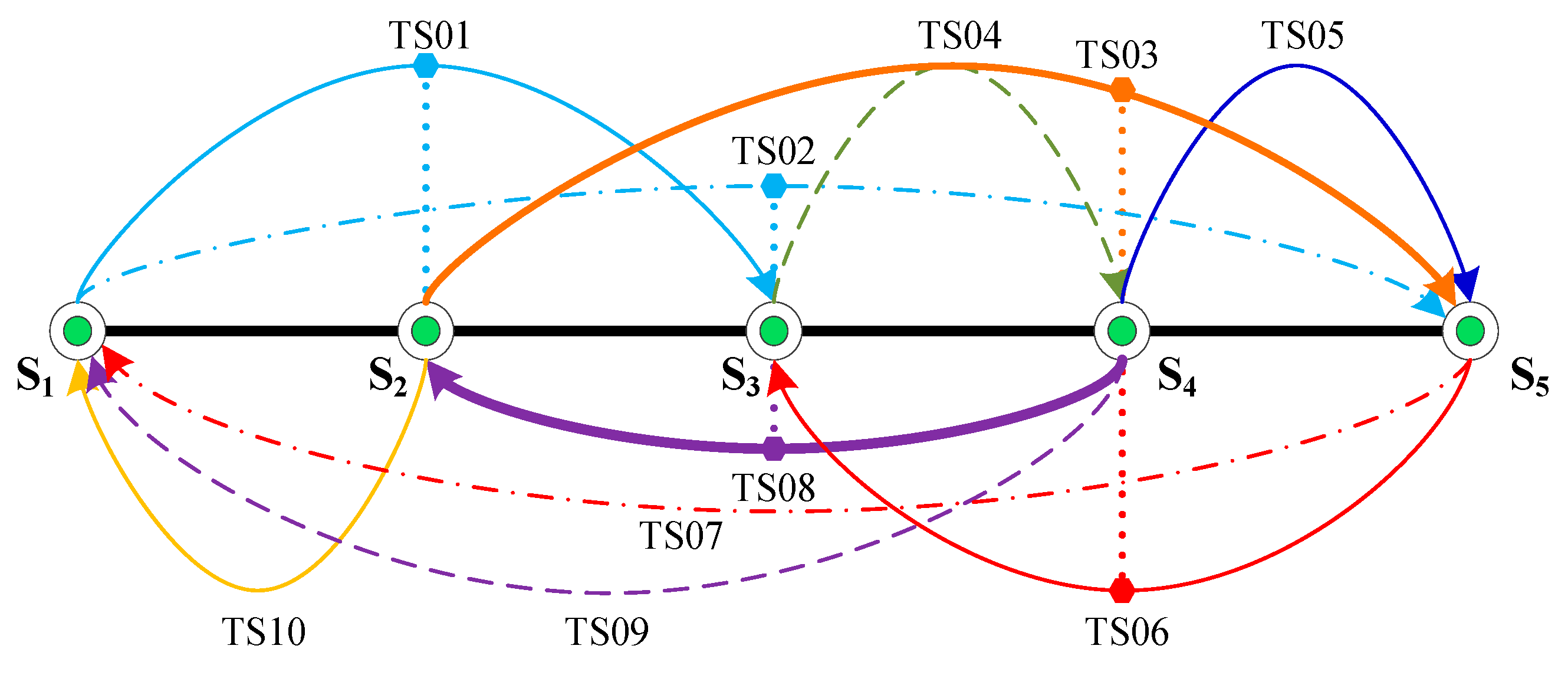
Figure 2.
A railway sub-network.

Figure 3.
The optimal service network.

Figure 4.
The impact of some key parameters on the total cost and number of trains dispatched.


Table 1.
Comparison between a few published studies and this work.
| Studies | Decision Variables | Constraints | Model Structure | Solution Approach | ||||
|---|---|---|---|---|---|---|---|---|
| Train Service | Service Frequency | Shipment Routing | Flow Conservation | Service Capacity | Transportation Time | |||
| Barnhart et al. (2000) | √ | × | √ | √ | √ | × | MIP | A heuristic Lagrangian relaxation |
| Campetella et al. (2006) | × | √ | √ | √ | √ | × | INLP | A heuristic algorithm based on tabu search |
| Ahuja et al. (2007) | √ | √ | √ | √ | √ | × | MIP | Very Large-scale Neighborhood Search |
| Ceselli et al. (2008) | √ | × | √ | √ | √ | √ | ILP | Column Generation |
| Lin et al. (2012) | √ | × | √ | √ | × | × | Bi-level | Simulated annealing |
| Zhu et al. (2014) | √ | × | √ | √ | √ | √ | MIP | A matheuristic solution integrating exact and meta-heuristic principles |
| This work | √ | √ | √ | √ | √ | √ | ILP | Gurobi/Simulated annealing |
Table 2.
Notations used in this paper.
| Sets | Definition |
| Set of stations in a rail network. | |
| Set of speed levels of train services. | |
| Set of stop strategies for express trains dispatched from to . | |
| Set of service arcs that might be provided from to , irrespective of the speed levels of the service. | |
| Set of service arcs leaving station . | |
| Set of service arcs entering station . | |
| Set of natural numbers. | |
| Parameters | Definition |
| Index of stations, . | |
| Index of speed levels of services, . | |
| Index of service arcs, . | |
| Index of stop strategies of services, . | |
| The th stop strategy for the train service provided from to , ; | |
| Train stop parameter, it takes value one if an express train dispatched from to with the th stop strategy stops at station . Otherwise, it is zero. In addition, if this train service is provided, then ; otherwise, . | |
| Service arc parameter, its value is one if the service arc exists when the train service with the th stop strategy is provided from to . Otherwise, it is zero. | |
| The number of cars which origin at station and are destined to . | |
| The fixed cost of dispatching an express train on a speed level of . | |
| The variable cost of a train on speed level per kilometer. | |
| The coefficient of converting car-hour cost into economic cost. | |
| The starting station of arc . | |
| The ending station of arc . | |
| The mileage from to . | |
| The mileage of service arc . | |
| The travel speed of an express train on speed level . | |
| The size of a train, i.e., the maximum number of railcars in a train. | |
| The transport cost of a loaded railcar per kilometer when the speed level is . | |
| The transfer cost of a railcar in average at station . | |
| The waiting cost of a railcar in average at station . | |
| The average transfer delay of a railcar when transferring at station . | |
| The average waiting delay of a railcar when waiting at station . | |
| The generalized transport cost of a railcar per kilometer at a speed level of . | |
| The generalized transfer cost of a railcar in average at station . | |
| The generalized waiting cost of a railcar in average at station . | |
| The maximum time consumption for a shipment which is specified in advance. | |
| A sufficiently large positive number. | |
| Decision Variables | Definition |
| Service selection variable; its value is one if the train service, whose speed level is and stop strategy is , is provided from to . Otherwise, it is zero. | |
| Service frequency variable; the number of trains dispatched from to per day, whose speed level is and stop strategy is . As express shipments are generally sensitive to the transportation time, at least one freight train will be dispatched for shipping the commodity in a day, if the shipment volume is positive. The value of this variable is an integer. | |
| Shipment routing variable; it takes a value of one if the shipment , i.e., the OD demand which originates at station and are destined to , is carried by service arc at a speed level of on its itinerary, where . Otherwise, it is zero. |
Table 3.
The input data.
| Stations | S1 | S2 | S3 | S4 | S5 |
|---|---|---|---|---|---|
| Shipment Volume (Cars Per Day) | |||||
| S1 | — | 11.7 | 9.5 | 10.1 | 2.3 |
| S2 | 12.6 | — | 14.7 | 17.7 | 8.1 |
| S3 | 8.7 | 12.9 | — | 8.8 | 10.7 |
| S4 | 7.8 | 15.4 | 9.7 | — | 11.3 |
| S5 | 4.5 | 13.1 | 7.2 | 7.6 | — |
| Transportation Time Constraint (Hours) | |||||
| S1 | — | 13.5 | 18.1 | 11.0 | 21.1 |
| S2 | 13.5 | — | 12.7 | 14.5 | 15.6 |
| S3 | 10.1 | 12.7 | — | 7.0 | 20.3 |
| S4 | 20.0 | 14.5 | 19.2 | — | 22.1 |
| S5 | 21.1 | 15.6 | 20.3 | 22.1 | — |
| Mileage of Each OD Pair (Kilometers) | |||||
| S1 | — | 439 | 811 | 960 | 1047 |
| S2 | 439 | — | 372 | 521 | 608 |
| S3 | 811 | 372 | — | 893 | 980 |
| S4 | 960 | 521 | 893 | — | 1129 |
| S5 | 1047 | 608 | 980 | 1129 | — |
| Generalized Transfer cost (CNY/car) | 20 | 18 | 22 | 19.2 | 20.8 |
| Transfer Delay (Hours) | 8 | 6 | 10 | 7.2 | 8.8 |
| Generalized Waiting cost (CNY/car) | 6 | 7.5 | 8 | 5 | 7 |
| Waiting Delay (Hours) | 2 | 2 | 3 | 1.5 | 2.5 |
Table 4.
The express services provided and shipment routing plans.
| No. | Train Service Origin to Destination | Speed Level | Intermediate Station | Stop Strategy | Service Frequency | Shipments Assigned to the Train Service |
|---|---|---|---|---|---|---|
| 1 | I | S2 | 1 | (S1, S2), (S1, S3), (S1, S5), (S2, S3) | ||
| 2 | II | S2 | 1 | (S1, S4), (S5, S4) | ||
| 3 | I | / | 1 | (S2, S4) | ||
| 4 | II | S2 | 1 | (S3, S1) | ||
| 5 | III | S2 | 1 | (S3, S4) | ||
| 6 | I | S2 | 1 | (S2, S5), (S3, S2), (S3, S5) | ||
| 7 | I | S2 | 1 | (S2, S1), (S4, S1), (S4, S2), (S5, S1) | ||
| 8 | I | S2 | 1 | (S1, S5), (S4, S3), (S4, S5) | ||
| 9 | I | / | 1 | (S5, S2) | ||
| 10 | I | S2 | 1 | (S4, S3), (S5, S1), (S5, S3), (S5, S4) |
Table 5.
The value of some critical parameters in the trials.
| Parameters | Standard Value | Step Size | Value in Trials |
|---|---|---|---|
| 5000 | 500 | 3500, 4000, 4500, 5000, 5500, 6000, 6500 | |
| 40 | 5 | 25, 30, 35, 40, 45, 50, 55 | |
| 5 | 0.5 | 3.5, 4, 4.5, 5, 5.5, 6, 6.5 | |
| 25 | 5 | 15, 20, 25, 30, 35, 40, 45 |
© 2018 by the authors. Licensee MDPI, Basel, Switzerland. This article is an open access article distributed under the terms and conditions of the Creative Commons Attribution (CC BY) license (http://creativecommons.org/licenses/by/4.0/).
Share and Cite
MDPI and ACS Style
Liu, S.; Lin, B.; Wu, J.; Zhao, Y. Modeling the Service Network Design Problem in Railway Express Shipment Delivery. Symmetry 2018, 10, 391. https://doi.org/10.3390/sym10090391
AMA Style
Liu S, Lin B, Wu J, Zhao Y. Modeling the Service Network Design Problem in Railway Express Shipment Delivery. Symmetry. 2018; 10(9):391. https://doi.org/10.3390/sym10090391
Chicago/Turabian StyleLiu, Siqi, Boliang Lin, Jianping Wu, and Yinan Zhao. 2018. "Modeling the Service Network Design Problem in Railway Express Shipment Delivery" Symmetry 10, no. 9: 391. https://doi.org/10.3390/sym10090391
Note that from the first issue of 2016, this journal uses article numbers instead of page numbers. See further details here.